Deep Semantic Segmentation of Natural and Medical Images: A Review
←
→
Page content transcription
If your browser does not render page correctly, please read the page content below
Springer Artificial Intelligence Review

                                        Deep Semantic Segmentation of Natural and Medical Images:
                                        A Review

                                        Saeid Asgari Taghanaki† · Kumar Abhishek† ·
                                        Joseph Paul Cohen · Julien Cohen-Adad · Ghassan
                                        Hamarneh

                                        Received: 20 December 2019 / Accepted: 25 May 2020
arXiv:1910.07655v3 [cs.CV] 3 Jun 2020

                                        Abstract The semantic image segmentation task consists of classifying each pixel of an
                                        image into an instance, where each instance corresponds to a class. This task is a part of the
                                        concept of scene understanding or better explaining the global context of an image. In the
                                        medical image analysis domain, image segmentation can be used for image-guided inter-
                                        ventions, radiotherapy, or improved radiological diagnostics. In this review, we categorize
                                        the leading deep learning-based medical and non-medical image segmentation solutions into
                                        six main groups of deep architectural, data synthesis-based, loss function-based, sequenced
                                        models, weakly supervised, and multi-task methods and provide a comprehensive review of
                                        the contributions in each of these groups. Further, for each group, we analyze each variant
                                        of these groups and discuss the limitations of the current approaches and present potential
                                        future research directions for semantic image segmentation.
                                        Keywords Semantic Image Segmentation · Deep Learning

                                        1 Introduction

                                        Deep learning has had a tremendous impact on various fields in science. The focus of the
                                        current study is on one of the most critical areas of computer vision: medical image anal-
                                        ysis (or medical computer vision), particularly deep learning-based approaches for medical
                                        image segmentation. Segmentation is an important processing step in natural images for
                                        scene understanding and medical image analysis, for image-guided interventions, radiother-
                                        apy, or improved radiological diagnostics, etc. Image segmentation is formally defined as
                                        †:   Joint first authors

                                        Saeid Asgari Taghanaki, Kumar Abhishek, and Ghassan Hamarneh
                                        School of Computing Science, Simon Fraser University, Canada
                                        E-mail: {sasgarit,kabhishe,hamarneh}@sfu.ca
                                        Joseph Paul Cohen
                                        Mila, Université de Montréal, Canada
                                        E-mail: joseph@josephpcohen.com
                                        Julien Cohen-Adad
                                        NeuroPoly Lab, Institute of Biomedical Engineering, Polytechnique Montréal, Canada
                                        E-mail: jcohen@polymtl.ca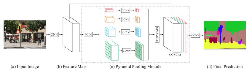
2                                                                           S. A. Taghanaki et al.

“the partition of an image into a set of nonoverlapping regions whose union is the entire
image” (Haralick and Shapiro, 1992). A plethora of deep learning approaches for medical
image segmentation have been introduced in the literature for different medical imaging
modalities, including X-ray, visible-light imaging (e.g. colour dermoscopic images), mag-
netic resonance imaging (MRI), positron emission tomography (PET), computerized tomog-
raphy (CT), and ultrasound (e.g. echocardiographic scans). Deep architectural improvement
has been a focus of many researchers for different purposes, e.g., tackling gradient vanishing
and exploding of deep models, model compression for efficient small yet accurate models,
while other works have tried to improve the performance of deep networks by introducing
new optimization functions.
     Guo et al. (2018) provided a review of deep learning based semantic segmentation of
images, and divided the literature into three categories: region-based, fully convolutional
network (FCN)-based, and weakly supervised segmentation methods. Hu et al. (2018b)
summarized the most commonly used RGB-D datasets for semantic segmentation as well
as traditional machine learning based methods and deep learning-based network architec-
tures for RGB-D segmentation. Lateef and Ruichek (2019) presented an extensive survey of
deep learning architectures, datasets, and evaluation methods for the semantic segmentation
of natural images using deep neural networks. Similarly, for medical imaging, Goceri and
Goceri (2017) presented an high-level overview of deep learning-based medical image anal-
ysis techniques and application areas. Hesamian et al. (2019) presented an overview of the
state-of-the-art methods in medical image segmentation using deep learning by covering the
literature related to network structures and model training techniques. Karimi et al. (2019)
reviewed the literature on techniques to handle label noise in deep learning based medi-
cal image analysis and evaluated existing approaches on three medical imaging datasets for
segmentation and classification tasks. Zhou et al. (2019b) presented a review of techniques
proposed for fusion of medical images from multiple modalities for medical image segmen-
tation. Goceri (2019a) discussed the fully supervised, weakly supervised and transfer learn-
ing techniques for training deep neural networks for segmentation of medical images, and
also discussed the existing methods for addressing the problems of lack of data and class im-
balance. Zhang et al. (2019) presented a review of the approaches to address the problem of
small sample sizes in medical image analysis, and divided the literature into five categories
including explanation, weakly supervised, transfer learning, and active learning techniques.
Tajbakhsh et al. (2020) presented a review of the literature for addressing the challenges of
scarce annotations as well as weak annotations (e.g., noisy annotations, image-level labels,
sparse annotations, etc.) in medical image segmentation. Similarly, there are several surveys
covering the literature on the task of object detection (Wang et al., 2019c; Zou et al., 2019;
Borji et al., 2019; Liu et al., 2019b; Zhao et al., 2019), which can also be used to obtain what
can be termed as rough localizations of the object(s) of interest. In contrast to the existing
surveys, we make the following contributions in this review:

    – We provide comprehensive coverage of research contributions in the field of semantic
      segmentation of natural and medical images. In terms of medical imaging modalities,
      we cover the literature pertaining to both 2D (RGB and grayscale) as well as volumetric
      medical images.
    – We group the semantic image segmentation literature into six different categories based
      on the nature of their contributions: architectural improvements, optimization function
      based improvements, data synthesis based improvements, weakly supervised models,
      sequenced models, and multi-task models. Figure 1 indicates the categories we cover
      in this review, along with a timeline of the most influential papers in the respective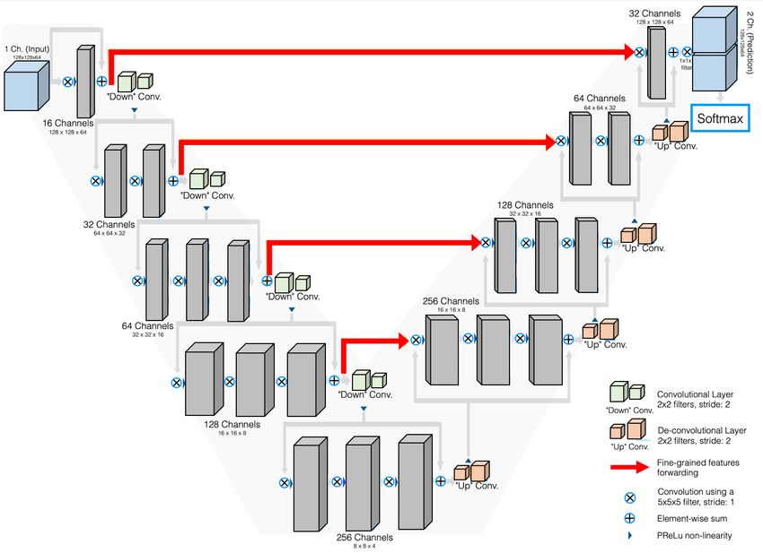
Deep Semantic Segmentation of Natural and Medical Images: A Review 3
categories. Moreover, Figure 2 shows a high-level overview of the deep semantic seg-
mentation pipeline, and where each of the categories mentioned in Figure 1 belong in
the pipeline.
– We study the behaviour of many popular loss functions used to train segmentation mod-
els on handling scenarios with varying levels of false positive and negative predictions.
– Followed by the comprehensive review, we recognize and suggest the important research
directions for each of the categories.
Sequenced
Adversarial Models
Training Cross Entropy Bounding Box
based Annotations
LSTM
Encoder- Computational
Decoder Complexity
Models Reduction Weakly
Model Optimization
Architecture Energy Image-level Supervised Unsupervised
Functions Overlap based
Minimization Labels Methods Learning
Sections 2, 3 Sections 4, 5
Section 7
Fully
Attention
Convolutional Distance Regularization
Models
Networks based Priors
Multi-Task Models
Section 8
GAN
Detection
Synthesis
LSTM
Synthesis based Methods Multi-Task Models
Sequenced Models Section 6 Section 8
Paired Unpaired
Image-to-Image Image-to-Image Tracking Classification
RNN Translation Translation
(a) Topics surveyed in this review.
Kuntimad and Ranganath, 1999
Badrinarayanan et al., 2015
Ronneberger et al., 2015
Reddick et al., 1997
Chaichulee et al., 2017
Kervadec et al., 2019b
Chartsias et al., 2017
Bischke et al., 2019
Perone et al., 2019
Chen et al., 2017a
Yang et al., 2017b
Salehi et al., 2017
Jégou et al., 2017
Long et al., 2015
Alom et al., 2019
Lin et al., 2017b
Noh et al., 2015
Liu et al., 2019a
Lee et al., 2019
He et al., 2017
2013 2016 2018
Shallow 2015 2017 2019
Models
Kim and Hwang, 2016
Zhang et al., 2018b,c
Berman et al., 2018b
Chen et al., 2018a,b
Drozdal et al., 2018
Milletari et al., 2016
Couprie et al., 2013
Jaeger et al., 2018
Huo et al., 2018
Yu et al., 2018b
Luc et al., 2016
Bai et al., 2018
(b) A timeline of the various contributions in deep learning based semantic segmentation of natural and
medical images. The contributions are colored according to their topics in (a) above.
Fig. 1: An overview of the deep learning based segmentation methods covered in this review.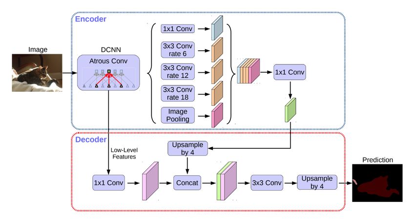
4                                                                                                    S. A. Taghanaki et al.

            Synthesis-based Methods
                    Section 6
                                                                             Model Architecture
                   (x, y)         (x’, y’)                                     Sections 2, 3

                                                                                                         Multi-Task Models
                                                              Input Space
                                                                                                              Section 8

                            (x, y)                              (x, y)                                           ŷ

     Pixel level        Image level
                                             No annotations
    annotations         annotations

    Supervised         Bounding box      Unsupervised
     Learning                              Learning                         Optimization Functions
                        annotations
                                                                                 Sections 4, 5
                     Semi-supervised
                        Learning

                     Weakly Supervised Methods
                             Section 7

Fig. 2: A typical deep neural network based semantic segmentation pipeline. Each compo-
nent in the pipeline indicates the section of this paper that covers the corresponding contri-
butions.

    In the following sections, we discuss deep semantic image segmentation improvements
under different categories visualized in Figure 1. For each category, we first review the im-
provements on non-medical datasets, and in a subsequent section, we survey the improve-
ments for medical images.

2 Network Architectural Improvements

This section discusses the advancements in semantic image segmentation using convolu-
tional neural networks (CNNs), which have been applied to interpretation tasks on both nat-
ural and medical images (Garcia-Garcia et al., 2018; Litjens et al., 2017). Although artificial
neural network-based image segmentation approaches have been explored in the past using
shallow networks (Reddick et al., 1997; Kuntimad and Ranganath, 1999) as well as works
which relied on superpixel segmentation maps to generate pixelwise predictions (Couprie
et al., 2013), in this work, we focus on deep neural network based image segmentation
models which are end-to-end trainable. The improvements are mostly attributed to explor-
ing new neural architectures (with varying depths, widths, and connectivity or topology) or
designing new types of components or layers.

2.1 Fully Convolutional Neural Networks for Semantic Segmentation

As one of the first high impact CNN-based segmentation models, Long et al. (2015) pro-
posed fully convolutional networks for pixel-wise labeling. They proposed up-sampling (de-
convolving) the output activation maps from which the pixel-wise output can be calculated.
The overall architecture of the network is visualized in Figure 3.
    In order to preserve the contextual spatial information within an image as the filtered
input data progresses deeper into the network, Long et al. (2015) proposed to fuse the output
with shallower layers’ output. The fusion step is visualized in Figure 4.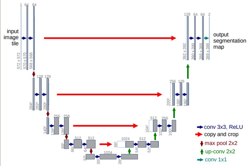
Deep Semantic Segmentation of Natural and Medical Images: A Review 5
Fig. 3: Fully convolutional networks can efficiently learn to make dense predictions for per-
pixel tasks like semantic segmentation (Long et al., 2015).
32x up-sampled 16x up-sampled 8x up-sampled
prediction (FCN-32s) prediction (FCN-32s) prediction (FCN-32s)
2x up-sampled 2x up-sampled
prediction prediction
Pool3 Pool4 Pool5
Fig. 4: Upsampling and fusion step of the fully convolution networks (Long et al., 2015).
2.2 Encoder-decoder Semantic Image Segmentation Networks
Next, encoder-decoder segmentation networks (Noh et al., 2015) such as SegNet, were in-
troduced (Badrinarayanan et al., 2015). The role of the decoder network is to map the low-
resolution encoder feature to full input resolution feature maps for pixel-wise classification.
The novelty of SegNet lies in the manner in which the decoder upsamples the lower resolu-
tion input feature maps. Specifically, the decoder uses pooling indices (Figure 5) computed
in the max-pooling step of the corresponding encoder to perform non-linear upsampling.
The architecture (Figure 5) consists of a sequence of non-linear processing layers (encoder)
and a corresponding set of decoder layers followed by a pixel-wise classifier. Typically, each
encoder consists of one or more convolutional layers with batch normalization and a ReLU
non-linearity, followed by non-overlapping max-pooling and sub-sampling. The sparse en-
coding due to the pooling process is upsampled in the decoder using the max-pooling indices
in the encoding sequence.
Ronneberger et al. (2015) proposed an architecture (U-Net; Figure 6) consisting of a
contracting path to capture context and a symmetric expanding path that enables precise lo-
calization. Similar to the image recognition (He et al., 2016) and keypoint detection (Honari
et al., 2016), Ronneberger et al. (2015) added skip connections to the encoder-decoder image
segmentation networks, e.g., SegNet, which improved the model’s accuracy and addressed
the problem of vanishing gradients.
Milletari et al. (2016) proposed a similar architecture (V-Net; Figure 7) which added
residual connections and replaced 2D operations with their 3D counterparts in order to pro-
cess volumetric images. Milletari et al. also proposed optimizing for a widely used segmen-
tation metric, i.e., Dice, which will be discussed in more detail in the section 4.
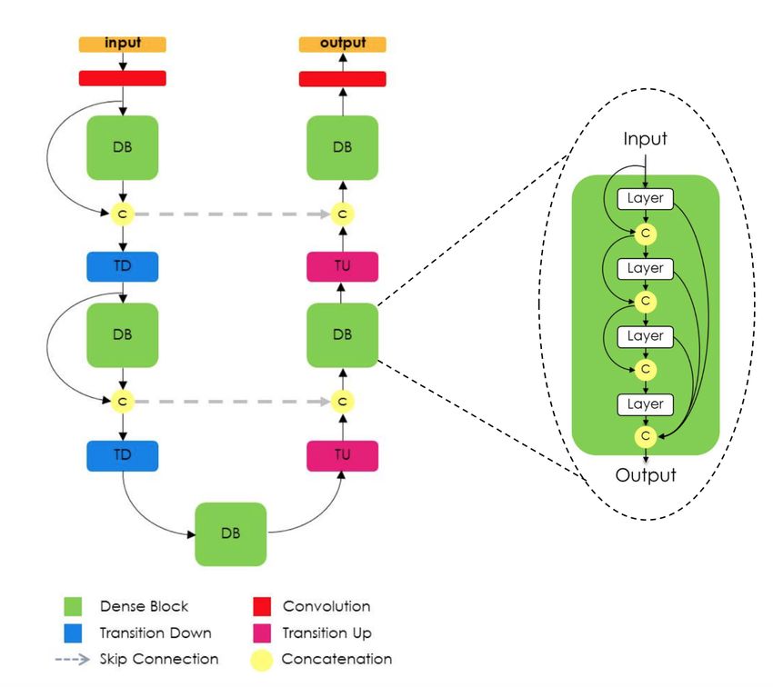
Jégou et al. (2017) developed a segmentation version of the densely connected networks
architecture (DenseNet (Huang et al. (2017)) by adapting the U-Net like encoder-decoder
skeleton. In Figure 8, the detailed architecture of the network is visualized.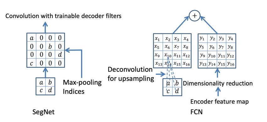
6                                                                         S. A. Taghanaki et al.

                                          Pooling
                                          indices

          Input                                                             Output

                                         Down sampling
                                        Conv + BN + Relu
                                          Up sampling

Fig. 5: Top: An illustration of the SegNet architecture. There are no fully connected lay-
ers, and hence it is only convolutional. Bottom: An illustration of SegNet and FCN (Long
et al., 2015) decoders. a, b, c, d correspond to values in a feature map. SegNet uses the
max-pooling indices to upsample (without learning) the feature map(s) and convolves with
a trainable decoder filter bank. FCN upsamples by learning to deconvolve the input feature
map and adds the corresponding encoder feature map to produce the decoder output. This
feature map is the output of the max-pooling layer (includes sub-sampling) in the corre-
sponding encoder. Note that there are no trainable decoder filters in FCN (Badrinarayanan
et al. (2015)).

        Fig. 6: An illustration of the U-Net (Ronneberger et al., 2015) architecture.

   In Figure 9, we visualize the simplified architectural modifications applied to the first
image segmentation network i.e. FCN.
   Several modified versions (e.g. deeper/shallower, adding extra attention blocks) of encoder-
decoder networks have been applied to semantic segmentation (Amirul Islam et al., 2017;
Deep Semantic Segmentation of Natural and Medical Images: A Review                            7

           Fig. 7: An illustration of the V-Net (Milletari et al., 2016) architecture.

                             Input               Output

                             Conv                Conv

                             Dense               Dense

                             Down                 Up

                             Dense               Dense

                             Down                  Up

                                       Dense

Fig. 8: Diagram of the one-hundred layers Tiramisu network architecture (Jégou et al.,
2017). The architecture is built from dense blocks. The architecture is composed of a down-
sampling path with two transitions down and an upsampling path with two transitions up.
A circle represents concatenation, and the arrows represent connectivity patterns in the net-
work. Gray horizontal arrows represent skip connections, where the feature maps from the
downsampling path are concatenated with the corresponding feature maps in the upsampling
path. Note that the connectivity pattern in the upsampling and the downsampling paths are
different. In the downsampling path, the input to a dense block is concatenated with its out-
put, leading to linear growth of the number of feature maps, whereas in the upsampling path,
it is not the case.

Fu et al., 2019b; Lin et al., 2017a; Peng et al., 2017; Pohlen et al., 2017; Wojna et al., 2017;
Zhang et al., 2018d). Recently in 2018, DeepLabV3+ (Chen et al., 2018b) has outperformed
8 S. A. Taghanaki et al.
Cross Entropy
Cross Entropy
Cross Entropy
Dice
Cross Entropy
FCN Seg-Net U-Net V-Net Tiramisu
Fig. 9: Gradual architectural improvements applied to FCN (Long et al., 2015) over time.
many state-of-the-art segmentation networks on PASCAL VOC 2012 (Everingham et al.,
2015) and Cityscapes (Cordts et al., 2016) datasets. Zhao et al. (2017b) modified the feature
fusing operation proposed by Long et al. (2015) using a spatial pyramid pooling module
or encode-decoder structure (Figure 10) are used in deep neural networks for semantic seg-
mentation tasks. The spatial pyramid networks are able to encode multi-scale contextual
information by probing the incoming features with filters or pooling operations at multi-
ple rates and multiple effective fields-of-view, while the latter networks can capture sharper
object boundaries by gradually recovering the spatial information.
Conv
Conv
Conv
Input Conv Pool
U
P Conv Output
Conv
Concatenation
Pyramid Pooling
Fig. 10: Overview of the pyramid scene parsing networks. Given an input image (a), feature
maps from last convolution layer are pulled (b), then a pyramid parsing module is applied
to harvest different sub-region representations, followed by upsampling and concatenation
layers to form the final feature representation, which carries both local and global context
information in (c). Finally, the representation is fed into a convolution layer to get the final
per-pixel prediction (d) Zhao et al. (2017b).
Chen et al. (2018b) proposed to combine the advantages from both dilated convolutions
and feature pyramid pooling. Specifically, DeepLabv3+, extends DeepLabv3 (Chen et al.
(2017b)) by adding a simple yet effective decoder module (Figure 11) to refine the segmen-
tation results, especially along object boundaries using dilated convolutions and pyramid
features.Deep Semantic Segmentation of Natural and Medical Images: A Review 9
Encoder
Conv 1x1
Conv 3x3
Rate 6
Conv 3x3
Input Dilated Conv Rate 12
Conv 1x1
Conv 3x3
Rate 18
Image
pooling
Decoder
Up-sample
Conv 1x1 Conv 3x3 Up-sample Output
Fig. 11: An illustration of the DeepLabV3+; The encoder module encodes multi-scale con-
textual information by applying atrous (dilated) convolution at multiple scales, while the
simple yet effective decoder module refines the segmentation results along object bound-
aries (Chen et al., 2018b).
2.3 Computational Complexity Reduction for Image Segmentation Networks
Several works have been done on reducing the time and the computational complexity of
deep classification networks (Howard et al., 2017; Leroux et al., 2018). A few other works
have attempted to simplify the structure of deep networks, e.g., by tensor factorization (Kim
et al., 2015), channel/network pruning (Wen et al., 2016), or applying sparsity to connec-
tions (Han et al., 2016). Similarly, Yu et al. (2018b) addressed the high computational cost
associated with high resolution feature maps in U-shaped architectures by proposing spatial
and context paths to preserve the rich spatial information and obtain a large receptive field.
A few methods have focused on the complexity optimization of deep image segmentation
networks. Similar to the work of Saxena and Verbeek (2016), Liu et al. (2019a) proposed
a hierarchical neural architecture search for semantic image segmentation by performing
both cell and network-level search and achieved comparable results to the state-of-the-art
results on the PASCAL VOC 2012 (Everingham et al., 2015) and Cityscapes (Cordts et al.,
2016) datasets. In contrast, Chen et al. (2018a) focused on searching the much smaller
atrous spatial pyramid pooling module using random search. Depth-wise separable con-
volutions (Sifre, 2014; Chollet, 2017) offer computational complexity reductions since they
have fewer parameters and have therefore also been used in deep segmentation models (Chen
et al., 2018b; Sandler et al., 2018).
Besides network architecture search, Srivastava et al. (2015) modified ResNet in a way
to control the flow of information through a connection. Lin et al. (2017a) adopted one step
fusion without filtering the channels.
2.4 Attention-based Semantic Image Segmentation
Attention can be viewed as using information transferred from several subsequent layer-
s/feature maps to select and localize the most discriminative (or salient) part of the input sig-10 S. A. Taghanaki et al.
nal. Wang et al. (2017a) added an attention module to the deep residual network (ResNet) for
image classification. Their proposed attention module consists of several encoding-decoding
layers. Hu et al. (2018a) proposed a selection mechanism where feature maps are first ag-
gregated using global average pooling and reduced to a single channel descriptor. Then an
activation gate is used to highlight the most discriminative features. Wang et al. (2018b)
proposed non-local operation blocks for encoding long range spatio-temporal dependencies
with deep neural networks that can be plugged into existing architectures. Fu et al. (2019a)
proposed dual attention networks that apply both spatial and channel-based attention opera-
tions.
Li et al. (2018) proposed a pyramid attention based network, for semantic segmentation.
They combined an attention mechanism and a spatial pyramid to extract precise dense fea-
tures for pixel labeling instead of complicated dilated convolution and artificially designed
decoder networks. Chen et al. (2016) applied attention to DeepLab (Chen et al., 2017a)
which takes multi-scale inputs.
2.5 Adversarial Semantic Image Segmentation
Goodfellow et al. (2014) proposed an adversarial approach to learn deep generative models.
Their generative adversarial networks (GANs) take samples z from a fixed (e.g., standard
Gaussian) distribution pz (z), and transform them using a deterministic differentiable deep
network p(.) to approximate the distribution of training samples x. Inspired by adversarial
learning, Luc et al. (2016) trained a convolutional semantic segmentation network along
with an adversarial network that discriminates segmentation maps coming either from the
ground truth or from the segmentation network. Their loss function is defined as
N
X
` (θs , θa ) = `mce (s (xn ) , yn )
n=1
(1)
− λ [`bce (a (xn , yn ) , 1) +`bce (a (xn , s (xn )) , 0)] ,
where θs and θa denote the parameters of the segmentation and adversarial model, respec-
tively. lbce and lmce are binary and multi-class cross-entropy losses, respectively. In this
setup, the segmentor tries to produce segmentation maps that are close to the ground truth,
i.e., which look more realistic.
The main models being used for image segmentation mostly follow encoder-decoder
architectures as U-Net. Recent approaches have shown that dilated convolutions and feature
pyramid pooling can improve the U-Net style networks. In Section 3, we summarize how
these methods and their modified counterparts have been applied to medical images.
3 Architectural Improvements Applied to Medical Images
In this section, we review the different architectural based improvements for deep learning-
based 2D and volumetric medical image segmentation.Deep Semantic Segmentation of Natural and Medical Images: A Review 11
3.1 Model Compression based Image Segmentation
To perform image segmentation in real-time and be able to process larger images or (sub)
volumes in case of processing volumetric and high-resolution 2D images such as CT, MRI,
and histopathology images, several methods have attempted to compress deep models. Weng
et al. (2019a) applied a neural architecture search method to U-Net to obtain a smaller net-
work with a better organ/tumor segmentation performance on CT, MR, and ultrasound im-
ages. Brügger et al. (2019) by leveraging group normalization (Wu and He, 2018) and leaky
ReLU function, redesigned the U-Net architecture in order to make the network more mem-
ory efficient for 3D medical image segmentation. Perone et al. (2018) and Bonta and Kiran
(2019) designed a dilated convolution neural network with fewer parameters as compared to
the original convolution-based one. Some other works (Xu et al., 2018; Paschali et al., 2019)
have focused on weight quantization of deep networks for making segmentation networks
smaller.
3.2 Encoder Decoder based Image Segmentation
Drozdzal et al. (2018) proposed to normalize input images before segmentation by applying
a simple CNN prior to pushing the images to the main segmentation network. They showed
improved results on electron microscopy segmentation, liver segmentation from CT, and
prostate segmentation from MRI scans. Gu et al. (2019) proposed using a dilated convolution
block close to the network’s bottleneck to preserve contextual information.
Vorontsov et al. (2019), using a dataset defined in Cohen et al. (2018), proposed an
image-to-image based framework to transform an input image with object of interest (pres-
ence domain) like a tumor to an image without the tumor (absence domain) i.e. translate dis-
eased image to healthy; next, their model learns to add the removed tumor to the new healthy
image. This results in capturing detailed structure from the object, which improves the seg-
mentation of the object. Zhou et al. (2018) proposed a rewiring method for the long skip
connections used in U-Net and tested their method on nodule segmentation in the low-dose
CT scans of the chest, nuclei segmentation in the microscopy images, liver segmentation in
abdominal CT scans, and polyp segmentation in colonoscopy videos.
3.3 Attention based Image Segmentation
Nie et al. (2018) designed an attention model to segment prostate from MRI images with
higher accuracy compared to baseline models, e.g., V-Net (Milletari et al., 2016) and FCN (Long
et al., 2015). Sinha and Dolz (2019) proposed a multi-level attention based architecture for
abdominal organ segmentation from MRI images. Qin et al. (2018) proposed a dilated con-
volution base block to preserve more detailed attention in 3D medical image segmentation.
Similarly, other papers (Lian et al., 2018; Isensee et al., 2019; Li et al., 2019b; Ni et al.,
2019; Oktay et al., 2018; Schlemper et al., 2019) have leveraged the attention concept into
medical image segmentation as well.
3.4 Adversarial Training based Image Segmentation
Khosravan et al. (2019) proposed an adversarial training framework for pancreas segmen-
tation from CT scans. Son et al. (2017) applied GANs for retinal image segmentation. Xue12 S. A. Taghanaki et al.
et al. (2018) used a fully convolutional network as a segmenter in the generative adversarial
framework to segment brain tumors from MRI images. Other papers (Costa et al., 2017; Dai
et al., 2018; Jin et al., 2018; Moeskops et al., 2017; Neff et al., 2017; Rezaei et al., 2017;
Yang et al., 2017a; Zhang et al., 2017) have also successfully applied adversarial learning to
medical image segmentation.
3.5 Sequenced Models
The Recurrent Neural Network (RNN) was designed for handling sequences. The long short-
term memory (LSTM) network is a type of RNN that introduces self-loops to enable the
gradient flow for long duration (Hochreiter and Schmidhuber, 1997). In the medical image
analysis domain, RNNs have been used to model the temporal dependency in image se-
quences. Bai et al. (2018) proposed an image sequence segmentation algorithm by combin-
ing a fully convolutional network with a recurrent neural network, which incorporates both
spatial and temporal information into the segmentation task. Similarly, Gao et al. (2018)
applied LSTM and CNN to model temporal relationship in brian MRI slices to improve
segmentation performance in 4D volumes. Li et al. (2019a) applied U-Net to obtain initial
segmentation probability maps and further improve them using LSTM for pancreas segmen-
tation from 3D CT scans. Similarly, other works have also applied RNNs (LSTMs) (Alom
et al., 2019; Chakravarty and Sivaswamy, 2018; Yang et al., 2017b; Zhao and Hamarneh,
2019a,b) to medical image segmentation.
4 Optimization Function based Improvements
In addition to improved segmentation speed and accuracy using architectural modifications
as mentioned in Section 2, designing new loss functions has also resulted in improvements
in subsequent inference-time segmentation accuracy.
4.1 Cross Entropy
The most commonly used loss function for the task of image segmentation is a pixel-wise
cross entropy loss (Eqn. 2). This loss examines each pixel individually, comparing the class
predictions vector to the one-hot encoded target (or ground truth) vector. For the case of
binary segmentation, let P (Y = 0) = p and P (Y = 1) = 1 − p. The predictions are given
by the logistic/sigmoid function P (Ŷ = 0) = 1+e1 −x = p̂ and P (Ŷ = 1) = 1 − 1+e1 −x =
1 − p̂, where x is output of network. Then cross entropy (CE) can be defined as:
CE(p, p̂) = −(p log(p̂) + (1 − p) log(1 − p̂)). (2)
The general form of the equation for multi-region (or multi-class) segmentation can be writ-
ten as:
X
CE = − p log p̂ (3)
classesDeep Semantic Segmentation of Natural and Medical Images: A Review 13
4.2 Weighted Cross Entropy
The cross-entropy loss evaluates the class predictions for each pixel vector individually and
then averages over all pixels, which implies equal learning to each pixel in the image. This
can be problematic if the various classes have unbalanced representation in the image, as
the most prevalent class can dominate training. Long et al. (2015) discussed weighting the
cross-entropy loss (WCE) for each class in order to counteract a class imbalance present in
the dataset. WCE was defined as:
WCE(p, p̂) = −(βp log(p̂) + (1 − p) log(1 − p̂)). (4)
To decrease the number of false negatives, β is set to a value larger than 1, and to
decrease the number of false positives β is set to a value smaller than 1. To weight the
negative pixels as well, the following balanced cross-entropy (BCE) can be used (Xie and
Tu, 2015).
BCE(p, p̂) = −(βp log(p̂) + (1 − β)(1 − p) log(1 − p̂)). (5)
Ronneberger et al. (2015) added a distance function to the cross-entropy function to
enforce learning distance between the components to enforce better segmentation in case of
having very close objects to each other as follows:
(d1 (x) + d2 (x))2
BCE(p, p̂) + w0 · exp − (6)
2σ 2
where d1 (x) and d2 (x) are two functions that calculate the distance to the border of nearest
and second cells in their cell segmentation problem.
4.3 Focal Loss
To reduce the contribution of easy examples so that the CNN focuses more on the difficult
examples, Lin et al. (2017b) added the term (1 − p̂)γ to the cross entropy loss as:
FL(p, p̂) = − (α(1 − p̂)γ p log(p̂) +(1 − α)p̂γ (1 − p) log(1 − p̂)) . (7)
Setting γ = 0 in this equation yields the BCE loss.
4.4 Overlap Measure based Loss Functions
4.4.1 Dice Loss / F1 Score
Another popular loss function for image segmentation tasks is based on the Dice coefficient,
which is essentially a measure of overlap between two samples and is equivalent to the F1
score. This measure ranges from 0 to 1, where a Dice coefficient of 1 denotes perfect and
complete overlap. The Dice coefficient (DC) is calculated as:
2T P 2|X ∩ Y |
DC = = . (8)
2T P + F P + F N |X|+|Y |14 S. A. Taghanaki et al.
Similarly, the Jaccard metric (intersection over union: IoU) is computed as:
TP |X ∩ Y |
IoU = = (9)
TP + FP + FN |X|+|Y |−|X ∩ Y |
where X and Y are the predicted and ground truth segmentation, respectively. TP is the true
positives, FP false positives and FN false negatives. We can see that DC ≥ IoU.
To use this as a loss function the DC can be defined as a Dice loss (DL) function (Mil-
letari et al., 2016):
2hp, p̂i
DL(p, p̂) = (10)
kpk1 +kp̂k1
where p ∈ {0, 1}n and 0 ≤ p̂ ≤ 1. p and p̂ are the ground truth and predicted segmentation
and h·, ·i denotes dot product.
4.4.2 Tversky Loss
Tversky loss (TL) (Salehi et al., 2017) is a generalization of the DL. To control the level of
FP and FN, TL weights them as the following:
hp, p̂i
TL(p, p̂) = (11)
hp, p̂i + β(1 − p, p̂i + (1 − β)(p, 1 − p̂)
setting β = 0.5 simplifies the equation to Eqn. 10.
4.4.3 Exponential Logarithmic Loss
Wong et al. (2018) proposed using a weighted sum of the exponential logarithmic Dice
loss (Leld ) and the weighted exponential cross-entropy loss (Lwece ) in order to improve the
segmentation accuracy on small structures for tasks where there is a large variability among
the sizes of the objects to be segmented.
L = weld Leld + wwece Lwece , (12)
where
Leld = E [(− ln (Di ))γD ] , and (13)
Lwece = E [(− ln (pl (x)))γCE ] . (14)
x, i, and l denote the pixel position, the predicted label, and the ground truth label. Di
denotes the smoothed Dice loss (obtained by adding an = 1 term to the numerator and
denominator in Eqn. 10 in order to handle missing labels while training, and γD and γCE
are used to control the non-linearities of the respective loss functions.Deep Semantic Segmentation of Natural and Medical Images: A Review 15
4.4.4 Lovász-Softmax loss
Since it has been shown that the Jaccard loss (IoU loss) is submodular (Berman et al.,
2018a), Berman et al. (2018b) proposed using the Lovász hinge with the Jaccard loss for bi-
nary segmentation, and proposed a surrogate of the Jaccard loss, called the Lovász-Softmax
loss, which can be applied for the multi-class segmentation task. The Lovász-Softmax loss
is, therefore, a smooth extension of the discrete Jaccard loss, and is defined as
1 X
LLovaszSoftmax = ∆Jc (m(c)) , (15)
|C|
c∈C
where ∆Jc (·) denotes the convex closure of the submodular Jaccard loss, · denotes that
it is a tight convex closure and polynomial time computable, C denotes all the classes, and
Jc and m(c) denote the Jaccard index and the vector of errors for class c respectively.
4.4.5 Boundary Loss
Kervadec et al. (2019a) proposed to calculate boundary loss LB along with the generalized
Dice loss LGD function as
αLGD (θ) + (1 − α)LB (θ), (16)
where the two terms in the loss function are defined as
P P
wG g(p)sθ (p) + wB p∈Ω (1 − g(p)) (1 − sθ (p))
LGD (θ) = 1 − 2 P p∈Ω P , and (17)
wG p∈Ω [sθ (p) + g(p)] + wB p∈Ω [2 − sθ (p) − g(p)]
LB (θ) = p ∈ ΩφG (p)sθ (p), (18)
where φG (p) = − kpP− z∂G (p)k if p ∈ G and φG (p) = kpP − z∂G (p)k, otherwise. The
general form integral Ω g(p)f (sθ (p)) is for foreground and Ω (1 − g(p))f (1 − sθ (p))
P 2
for background. wG = 1/ p∈Ω g(p) and
P 2
wB = 1/ Ω (1 − g(p)) .Ω shows the spatial domain.
4.4.6 Conservative Loss
Zhu et al. (2018) proposed the Conservative Loss for in order to achieve a good generaliza-
tion ability in domain adaptation tasks by penalizing the extreme cases and encouraging the
moderate cases. The Conservative Loss is defined as
CL(pt ) = λ(1 + loga (pt ))2 ∗ loga (− loga (pt )), (19)
where pt is the probability of the prediction towards the ground truth and a is the base of
the logarithm. a and λ are empirically chosen to be e (Euler’s number) and 5 respectively.
Other works also include approaches to optimize the segmentation metrics (Nowozin,
2014), weighting the loss function (Roy et al., 2017), and adding regularizers to loss func-
tions to encode geometrical and topological shape priors (BenTaieb and Hamarneh, 2016;
Mirikharaji and Hamarneh, 2018).16 S. A. Taghanaki et al.
Foreground Background False Negative False Positive
Fig. 12: A comparison of seven loss functions for different extends of overlaps for a large
(left) and a small (right) object.
A significant problem in image segmentation (particularly in medical images) is to over-
come class imbalance for which overlap measure based methods have shown reasonably
good performance in overcoming the imbalance. In Section 5, we summarize the approaches
which use new loss functions, particularly for medical image segmentation or use the (mod-
ified) loss functions mentioned above.
In Figure 12, we visualize the behavior of different loss functions for segmenting large
and small objects. For the parameters of the loss functions, we use the same parameters as
reported by the authors in their respective papers. Therefore, we use β = 0.3 in Eqn. 11,
α = 0.25 and γ = 2 in Eqn. 7, and γD = γCE = 1, weld = 0.8, and wwece = 0.2 in
Eqn. 12. Moving from the left to the right for each plot, the overlap of the predictions and
ground truth mask becomes progressively smaller, i.e., producing more false positives and
false negatives. Ideally, the loss value should monotonically increase as more false positives,
and negatives are predicted. For large objects, almost all the functions follow this assump-
tion; however, for the small objects (right plot), only combo loss and focal loss penalize
monotonically more for larger errors. In other words, the overlap-based functions highly
fluctuate while segmenting small and large objects (also see Figure 13), which results in un-
stable optimization. The loss functions which use cross-entropy as the base and the overlap
measure functions as a weighted regularizer show more stability during training.
5 Optimization Function based Improvements Applied to Medical Images
The standard CE loss function and its weighted versions, as discussed in Section 4, have been
applied to numerous medical image segmentation problems (Isensee et al., 2019; Li et al.,
2019b; Lian et al., 2018; Ni et al., 2019; Nie et al., 2018; Oktay et al., 2018; Schlemper et al.,
2019). However, Milletari et al. (2016) found that optimizing CNNs for DL (Eqn. 10) in
some cases, e.g., in the case of having very small foreground objects in a large background,
works better than the original cross-entropy.
Li et al. (2019c) proposed adding the following regularization term to the cross entropy
loss function to encourage smooth segmentation outputs.Deep Semantic Segmentation of Natural and Medical Images: A Review 17
Fig. 13: Comparison of cross entropy and Dice losses for segmenting small and large ob-
jects. The red pixels show the ground truth and the predicted foregrounds in the left and right
columns respectively. The striped and the pink pixels indicate false negative and false posi-
tive, respectively. For the top row (i.e., large foreground), the Dice loss returns 0.96 for one
false negative and for the bottom row (i.e., small object) returns 0.66 for one false negative,
whereas the cross entropy loss function outputs 0.83 for both the cases. By considering a
false negative and false positive, the output value drops even more in case of using Dice but
the cross entropy stays smooth (i.e., Dice value of 0.93 and 0.50 for large and small object
versus cross entropy loss value of 1.66 for both.)
N
2
Eξ0 ,ξ f xi ; θ, ξ 0 − f (xi ; θ, ξ)
X
R= (20)
i=1
where ξ 0 and ξ are different perturbation (e.g., Gaussian noise, network dropout, and ran-
domized data transformation) applied to the input image xi .
Chen et al. (2019) proposed leveraging traditional active contour energy minimization
into CNNs via the following loss function.
Loss = Length +λ · Region (21)
i=1,j=1 r
X 2 2
Length = ∇uxi,j + ∇uyi,j + (22)
Ω
where x and y from uxi,j and uyi,j are horizontal and vertical directions, respectively.
i=1,j=1
X i=1,j=1
X
Region = ui,j (c1 − vi,j )2 + (1 − ui,j ) (c2 − vi,j )2 (23)
Ω Ω
where u and v are represented as prediction and a given image, respectively. c1 is set to 1
and c2 to 0. Similar to, Li et al. (2019c), Zhou et al. (2019a) proposed adding a contour
regression term to the weighted cross entropy loss function.
Karimi and Salcudean (2019) optimized Hausdorff distance based function between a
predicted and ground truth segmentation as follows.
P
2 (p ◦ q)
fHD (p, q) = Loss(p, q) + λ 1 − P Ω 2 2
(24)
Ω (p + q )
where the second term is the Dice loss function and the first term can be replaced with
three different versions of the Hausdorff distance for p and q i.e. ground truth and predicted
segmentations respectively, as follows;18 S. A. Taghanaki et al.
1 X
Loss(q, p) = (p − q)2 ◦ dα α
p + dq (25)
|Ω|
Ω
The parameter α determines the level of penalty for larger errors. dp is the distance map
of the ground-truth segmentation as the unsigned distance to the boundary δp. Similarly, dq
is defined as the distance to δq. The ◦ is Hadamard operation.
K
1 X X
Loss(q, p) = (p − q)2 k B kα (26)
|Ω|
k=1 Ω
where k denotes k successive erosions. where
0 1/5 0
B = 1/5 1/5 1/5 (27)
0 1/5 0
1 X α Xh
Loss(q, p) = r fs Br ∗ pC ◦ fq\p + fs (Br ∗ p) ◦ fp\q
|Ω|
r∈R Ω (28)
C
+ fs B r ∗ q ◦ fp\q + fs (Br ∗ q) ◦ fq\p ]
where fq\p = (p − q)2 q. fs indicates soft thresholding. Br denotes a circular-shaped
convolutional kernel of radius r. Elements of Br are normalized such that they sum to one.
pC = 1 − p. Ground-truth and predicted segmentations, denoted with p and q,
Caliva et al. (2019) proposed to measure distance of each voxel to the boundaries of the
objects and use the weight matrices to penalize a model for error on the boundaries. Kim and
Ye (2019) proposed using level-set energy minimization as a regularizer summed with stan-
dard multi-class cross entropy loss function for semi-supervised brain MRI segmentation
as:
N Z N Z
X 2 X
Llevel (Θ; x) = x(r) − cΘ
n
Θ
yn (r)dr + λ Θ
∇yn (r) dr (29)
n=1 Ω n=1 Ω
with
Θ
R
x(r)yn (r)dr
cΘ
n = ΩR
Θ
(30)
y (r)dr
Ω n
Θ
where x(r) is the input, yn (r) is the output of softmax layer, Θ refers to learnable
parameters.
Taghanaki et al. (2019e) discussed the risks of using solo overlap based loss functions
and proposed to use them as regularizes along with a weighted cross entropy to explicitly
handle input and output imbalance as follows;
N
1 X
Combo Loss = α − β (ti − ln pi ) + (1 − β) [(1 − ti ) ln (1 − pi )]
N
i=1
K
!
2 N
P
i=1 pi ti + S
X
+ (1 − α) − PN PN (31)
i=1 i=1 pi + i=1 ti + SDeep Semantic Segmentation of Natural and Medical Images: A Review 19
where α controls the amount of Dice term contribution in the loss function L, and β ∈ [0, 1]
controls the level of model penalization for false positives/negatives: when β is set to a
value smaller than 0.5, F P are penalized more than F N as the term (1 − ti ) ln (1 − pi ) is
weighted more heavily, and vice versa. In their implementation, to prevent division by zero,
the authors perform add-one smoothing (a specific instance of the additive/Laplace/Lidstone
smoothing; Russell and Norvig (2016)), i.e., they add unity constant S to both the denomi-
nator and numerator of the Dice term.
The majority of the methods discussed in Section 5 have attempted to handle the class
imbalance issue in the input images i.e., small foreground versus large background with
providing weights/penalty terms in the loss function. Other approaches consist of first iden-
tifying the object of interest, cropping around this object, and then performing the task (e.g.,
segmentation) with better-balanced classes. This type of cascade approach has been applied
for the segmentation of multiple sclerosis lesions in the spinal cord (Gros et al., 2019).
6 Image Synthesis based Methods
Deep CNNs are heavily reliant on big data to avoid overfitting and class imbalance issues,
and therefore this section focuses on data augmentation, a data-space solution to the problem
of limited data. Apart from standard online image augmentation methods such as geomet-
ric transformations (LeCun et al., 1998; Simard et al., 2003; Cireşan et al., 2011, 2012;
Krizhevsky et al., 2012), color space augmentations (Galdran et al., 2017; Yuan, 2017; Ab-
hishek et al., 2020), etc., in this section, we discuss image synthesis methods, the output
of which are novel images rather than modifications to existing images. GANs based aug-
mentation techniques for segmentation tasks have been used for a wide variety of problems
- from remote sensing imagery (Mohajerani et al., 2019) to filamentary anatomical struc-
tures (Zhao et al., 2017a). For a more detailed review of image augmentation strategies in
deep learning, we direct the interested readers to Shorten and Khoshgoftaar (2019).
6.1 Image Synthesis based Methods Applied to Natural Image Segmentation
Neff et al. (2018) trained a Wasserstein GAN with gradient penalty (Gulrajani et al., 2017)
to generate labeled image data in the form of image-segmenation mask pairs. They eval-
uated their approach on a dataset of chest X-ray images and the Cityscapes dataset, and
found that the WGAN-GP was able to generate images with sufficient variety and that a
segmentation model trained using GAN-based augmentation only was able to perform bet-
ter than a model trained with geometric transformation based augmentation. Cherian and
Sullivan (2019) proposed to incorporate semantic consistency in image-to-image transla-
tion task by introducing segmentation functions in the GAN architecture and showed that
the semantic segmentation models trained with synthetic images led to considerable per-
formance improvements. Other works include GAN-based data augmentation for domain
adaptation (Huang et al., 2018; Choi et al., 2019) and panoptic data augmentation (Liu
et al., 2019c). However, the majority of GAN based data augmentation has been applied to
medical images (Shorten and Khoshgoftaar, 2019). Next, we discuss the GAN based image
synthesis for augmentation in the field of medical image analysis.20 S. A. Taghanaki et al. 6.2 Image Synthesis based Methods Applied to Medical Image Segmentation Chartsias et al. (2017) used a conditional GAN to generate cardiac MR images from CT images. They showed that utilizing the synthetic data increased the segmentation accuracy and that using only the synthetic data led to only a marginal decrease in the segmentation accuracy. Similarly, Zhang et al. (2018c) proposed a GAN based volume-to-volume trans- lation for generating MR volumes from corresponding CT volumes and vice versa. They showed that synthetic data improve segmentation performance on cardiovascular MRI vol- umes. Huo et al. (2018) proposed an end-to-end synthesis and segmentation network called EssNet to simultaneously synthesize CT images from unpaired MR images and to segment CT splenomegaly on unlabeled CT images and showed that their approach yielded better segmentation performance than even segmentation obtained using models trained using the manual CT labels. Abhishek and Hamarneh (2019) trained a conditional GAN to generate skin lesion images from and confined to binary masks, and showed that using the synthe- sized images led to a higher skin lesion segmentation accuracy. Zhang et al. (2018b) trained a GAN for translating between digitally reconstructed radiographs and X-ray images and achieved similar accuracy as supervised training in multi-organ segmentation. Shin et al. (2018) proposed a method to generate synthetic abnormal MRI images with brain tumors by training a GAN using two publicly available data sets of brain MRI. Similarly, other works (Han et al., 2019; Yang et al., 2018; Yu et al., 2018a) have leveraged GANs to syn- thesize brain MR images. 7 Weakly Supervised Methods Collecting large-scale accurate pixel-level annotation is time-consuming and financially ex- pensive. However, unlabeled and weakly-labeled images can be collected in large amounts in a relatively fast and cheap manner. As shown in Figure 2, varying levels of supervision are possible when training deep segmentation models, from pixel-wise annotations (super- vised learning) and image-level and bounding box annotations (semi-supervised learning) to no annotations at all (unsupervised learning), the last two of which comprise weak su- pervision. Therefore, a promising direction for semantic image segmentation is to develop weakly supervised segmentation models. 7.1 Weakly Supervised Methods Applied to Natural Images Kim and Hwang (2016) proposed a weakly supervised semantic segmentation network using unpooling and deconvolution operations, and used feature maps from the deconvolutions layers to learn scale-invariant features, and evaluated their model on the PASCAL VOC and chest X-ray image datasets. Lee et al. (2019) used dropout (Srivastava et al., 2014) to choose features at random during training and inference and combine the many different localization maps to generate a single localization map, effectively discovering relationships between locations in an image, and evaluated their proposed approach on the PASCAL VOC dataset.
Deep Semantic Segmentation of Natural and Medical Images: A Review                         21

7.2 Weakly Supervised Methods Applied to Medical Images

The scarcity of richly annotated medical images is limiting supervised deep learning-based
solutions to medical image analysis tasks (Perone and Cohen-Adad, 2019), such as local-
izing discriminatory radiomic disease signatures. Therefore, it is desirable to leverage un-
supervised and weakly supervised models. Kervadec et al. (2019b) introduced a differen-
tiable term in the loss function for datasets with weakly supervised labels, which reduced
the computational demand for training while also achieving almost similar performance to
full supervision for segmentation of cardiac images. Afshari et al. (2019) used a fully con-
volutional architecture along with a Mumford-Shah functional Mumford and Shah (1989)
inspired loss function to segment lesions from PET scans using only bounding box anno-
tations as supervision. Mirikharaji et al. (2019) proposed to learn spatially adaptive weight
maps to account for spatial variations in pixel-level annotations and used noisy annotations
to train a segmentation model for skin lesions. Taghanaki et al. (2019d) proposed to learn
spatial masks using only image-level labels with minimizing mutual information between
the input and masks, and at the same time maximizing the mutual information between
the masks and image labels. Peng et al. (2019) proposed an approach to train a CNN with
discrete constraints and regularization priors based on the alternating direction method of
multipliers (ADMM). Perone and Cohen-Adad (2018) expanded the semi-supervised mean
teacher (Tarvainen and Valpola, 2017) approach to segmentation tasks on MRI data, and
show that it can bring important improvements in a realistic small data regime. In another
work, Perone et al. (2019) extended the method of unsupervised domain adaptation using
self-ensembling for the semantic segmentation task. They showed how this approach could
improve the generalization of the models even when using a small amount of unlabeled data.

8 Multi-Task Models

Multi-task learning (Caruana, 1997) refers to a machine learning approach where multiple
tasks are learned simultaneously, and the learning efficiency and the model performance
on each of the tasks are improved because of the existing commonalities across the tasks.
For visual recognition tasks, it has been shown that there exist relations between various
tasks in the task space (Zamir et al., 2018), and multi-task models can help exploit these
relationships to improve performance on the related tasks.

8.1 Multi-Task Models Applied to Natural Images

Bischke et al. (2019) proposed a cascaded multi-task loss to preserve boundary information
from segmentation masks for segmenting building footprints and achieved state-of-the-art
performance on an aerial image labeling task. He et al. (2017) extended Faster R-CNN (Ren
et al., 2015) by adding a new branch to predict the object mask along with a class label
and a bounding box, and the proposed model was called Mask R-CNN. Mask R-CNN has
been used extensively for multi-task segmentation models for a wide range of application
areas (Abdulla, 2017), such as adding sports fields to OpenStreetMap (Remillard, 2018), de-
tection and segmentation for surgery robots (SUYEgit, 2018), understanding climate change
patterns from aerial imagery of the Arctic (Zhang et al., 2018a), converting satellite imagery
to maps (Mohanty, 2018), detecting image forgeries (Wang et al., 2019d), and segmenting
tree canopy (Zhao et al., 2018).
22                                                                          S. A. Taghanaki et al.

8.2 Multi-Task Models Applied to Medical Images

Chaichulee et al. (2017) extended the VGG16 architecture (Simonyan and Zisserman, 2014)
to include a global average pooling layer for patient detection and a fully convolutional net-
work for skin segmentation. The proposed model was evaluated on images from a clinical
study conducted at a neonatal intensive care unit, and was robust to changes in lighting, skin
tone, and pose. He et al. (2019) trained a U-Net (Ronneberger et al., 2015)-like encoder-
decoder architecture to simultaneously segment thoracic organs from CT scans and perform
global slice classification. Ke et al. (2019) trained a multi-task U-Net architecture to solve
three tasks - separating wrongly connected objects, detecting class instances, and pixel-
wise labeling for each object, and evaluated it on a food microscopy image dataset. Other
multi-task models have also been proposed for segmentation and classification for detecting
manipulated faces in images and video (Nguyen et al., 2019) and diagnosis of breast biopsy
images (Mehta et al., 2018) and mammograms (Le et al., 2019).
     Mask R-CNN has also been used for segmentation tasks in medical image analysis such
as automatically segmenting and tracking cell migration in phase-contrast microscopy (Tsai
et al., 2019), detecting and segmenting nuclei from histological and microscopic images (John-
son, 2018; Vuola et al., 2019; Wang et al., 2019a,b), detecting and segmenting oral dis-
eases (Anantharaman et al., 2018), segmenting neuropathic ulcers (Gamage et al., 2019),
and labeling and segmenting ribs in chest X-rays (Wessel et al., 2019). Mask R-CNN has
also been extended to work with 3D volumes and has been evaluated on lung nodule de-
tection and segmentation from CT scans and breast lesion detection and categorization on
diffusion MR images (Jaeger et al., 2018; Kopelowitz and Engelhard, 2019).

9 Segmentation Evaluation Metrics and Datasets

9.1 Evaluation Metrics

The quantitative evaluation of segmentation models can be performed using pixel-wise and
overlap based measures. For binary segmentation, pixel-wise measures involve the construc-
tion of a confusion matrix to calculate the number of true positive (TP), true negative (TN),
false positive (FP), and false negative (FN) pixels, and then calculate various metrics such
as precision, recall (also known as sensitivity), specificity, and overall pixel-wise accuracy.
They are defined as follows:

                                                  TP
                                  Precision =           ,                                   (32)
                                                TP + FP
                                                        TP
                            Recall or Sensitivity =           ,                             (33)
                                                      TP + FN
                                               TN
                             Specificity =           ,      and,                            (34)
                                             TN + FP
                                             TP + TN
                          Accuracy =                      .                                 (35)
                                        TP + TN + FP + FN
    Two popular overlap-based measures used to evaluate segmentation performance are the
SørensenDice coefficient (also known as the Dice coefficient) and the Jaccard index (also
known as the intersection over union or IoU). Given two sets A and B, these metrics are
defined as:
Deep Semantic Segmentation of Natural and Medical Images: A Review 23
|A ∩ B|
Dice coefficient, Dice(A, B) = 2 , and, (36)
|A| + |B|
|A ∩ B|
Jaccard index, Jaccard(A, B) = . (37)
|A ∪ B|
For binary segmentation masks, these overlap-based measures can also be calculated
from the confusion matrix as shown in Equations 8 and 9 respectively. The two measures
are related by:
Dice
Jaccard = . (38)
2 − Dice
(a) Ground truth binary mask (b) Predicted binary mask (c) Overlap between the masks.
Fig. 14: A 5 × 5 overlap scenario with (a) the ground truth, (b) the predicted binary masks,
and (c) the overlap. In (a) and (b), black and white pixels denote the foreground and the
background respectively. In (c), green, grey, blue, and red pixels denote TP, TN, FP, and FN
pixels respectively.
Figure 14 contains a simple overlap scenario, with the ground truth and the predicted
binary masks with a spatial resolution 5 × 5. Let black pixels denote the object to be seg-
mented. The confusion matrix for this can be constructed as shown in Table 1. Using the ex-
7
pressions above, we can calculate the metrics as precision = 87 = 0.875, recall = 10 = 0.7,
14
specificity = 15 = 0.9333, pixel-wise accuracy = 21 25 = 0.84, Dice coefficient = 79 =
7
0.7778, and Jaccard index = 11 = 0.6364.
Table 1: Confusion matrix for the overlap scenario shown in Figure 14.
Ground Truth
Background Object
Background 14 3
Prediction
Object 1 7
9.2 Semantic Segmentation Datasets for Natural Images
Next, we briefly discuss the most popular and widely used datasets for the semantic segmen-
tation of natural images. These datasets cover various categories of scenes, such as indoor
and outdoor environments, common objects, urban street view as well as generic scenes. For
a comprehensive review of the natural image datasets that segmentation models are usually
benchmarked upon, we direct the interested readers to Lateef and Ruichek (2019).You can also read