Demand Shaping in Cellular Networks - arXiv
←
→
Page content transcription
If your browser does not render page correctly, please read the page content below
1

                                                               Demand Shaping in Cellular Networks
                                                                                               Xinyang Zhou                       Lijun Chen

                                              Abstract— Demand shaping is a promising way to mitigate
                                           the wireless cellular capacity shortfall in the presence of ever-
                                           increasing wireless data demand. In this paper, we formulate
                                           demand shaping as an optimization problem that minimizes
                                           the variation in aggregate traffic. We design a distributed and
                                           randomized offline demand shaping algorithm under complete
arXiv:1707.02503v2 [math.OC] 27 Mar 2018

                                           traffic information and prove its almost surely convergence.
                                           We further consider a more realistic setting where the traffic
                                           information is incomplete but the future traffic can be predicted
                                           to a certain degree of accuracy. We design an online demand
                                           shaping algorithm that updates the schedules of deferrable
                                           applications (DAs) each time when new information is available,
                                           based on solving at each timeslot an optimization problem over
                                           a shrinking horizon from the current time to the end of the day.
                                           We compare the performance of the online algorithm against                       Fig. 1: North America smartphone web browsing activity in
                                           the optimal offline algorithm, and provide numerical examples
                                                                                                                            one day [21].
                                           to complement the theoretical analysis.
                                             Index Terms— Demand shaping, offline algorithm, online al-                     web browsing activity over a day. However, wireless capacity
                                           gorithm, steepest descent algorithm, supermartingale, deferrable
                                                                                                                            needs to be provisioned to meet the peak demand rather than
                                           applications, cellular networks.
                                                                                                                            the average. This means that the cellular network is usually
                                                                                                                            stressed in peak hours while largely underutilized at other
                                                                     I. I NTRODUCTION                                       times. If the demand profile can be shaped to reduce the peak
                                              We have witnessed in recent years rapid increase in demand                    and smooth the time variation, not only can more traffic be
                                           for wireless data, driven by the proliferation of smart mobile                   accommodated under limited existing capacity constraints, but
                                           devices. The global mobile traffic in 2016 has nearly reached                    also additional spectrum allocation and infrastructure upgrades
                                           84 exabytes, more than 80 times greater than the entire global                   can be slowed down, which together greatly improve wireless
                                           Internet traffic in 2000; yet, this number is expected to be                     network efficiency and QoS, and yield huge savings for service
                                           increasing at a compound annual growth rate (CAGR) of 47%                        providers.
                                           in the coming five years, i.e., a seven-fold growth from 2016                       In this paper, we focus on designing demand shaping
                                           to 2021 [20]. However, despite frequent upgrades of cellular                     algorithms for cellular networks. We divide wireless traffic into
                                           networks technology from 2G to 4G LTE and beyond, wireless                       two categories: non-deferrable traffic and deferrable traffic.
                                           service providers fall short of keeping up with this increasing                  Non-deferrable traffic refers to the traffic of those applications
                                           wireless data demand, leading to congestion in the network,                      such as online gaming that have no or low delay tolerance, and
                                           especially in areas of dense population. As a result, users’ data                constitutes the base traffic whose profile cannot be shaped.
                                           rates have to be throttled to ease congestions [2], [6], [9], at                 Deferrable traffic refers to the traffic of those applications
                                           the cost of the degraded quality of service (QoS).                               such as file uploading/downloading that are flexible in time
                                              Admittedly, the capacity shortfall of cellular networks can                   and only require being served by a designated deadline, e.g.,
                                           be mitigated by allocating more wireless spectrum and deploy-                    finishing photo backup on cellphone by 12 am. Deferrable
                                           ing more wireless infrastructures including more and smaller                     applications (DAs) are further divided into two major types:
                                           cells and WiFi networks offloading, etc. However, spectrum                       (1) continuous-rate interruptible applications such as photos
                                           allocation and infrastructure upgrading are not only costly but                  backup and applications update that allow any data rates—
                                           also time-consuming, while WiFi networks may not always be                       e.g., the delayed offloading in [27], [30], and (2) discrete-rate
                                           available and secure. A promising alternative, inspired by the                   non-interruptible applications such as online movie streaming
                                           similar problem of demand response in power networks, is to                      and video conference that usually require certain constant data
                                           improve spectrum and infrastructure efficiency through man-                      rate [3], [4] and should not be interrupted once started, e.g.,
                                           aging wireless data traffic (i.e., demand). Notice that wireless                 one can schedule movie watching or video conference to the
                                           traffic or demand usually fluctuates with a large peak-to-valley                 “valley” time to enjoy better graphic quality and incur less
                                           ratio throughout a day; see Fig. 1 for a trace of smartphone                     data cost if he/she has the time flexibility. See Table I for a
                                              X. Zhou and L. Chen are with College of Engineering and Applied Science,      summary of traffic types and examples. We seek to schedule
                                           University of Colorado, Boulder, CO 80309, USA (emails: {xinyang.zhou,           the deferrable traffic to flatten the aggregate traffic profile over
                                           lijun.chen}@colorado.edu).                                                       a day.
                                              Preliminary result of this paper has been presented at the Allerton Confer-
                                           ence on Communication, Control, and Computing, Monticello, Illinois, 2014           Specifically, we formulate the cellular traffic demand shap-
                                           [39].                                                                            ing as an optimization problem that minimizes the (time)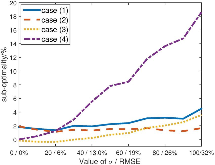
2

         Traffic/Application Type                     Examples
       Non-deferrable application          Online gaming, web browsing
                                                                              future demand and renewable energy supply, and Parise et al
    Discrete-rate non-interruptible DA   Movie streaming, video conference    [31] that proposes a decentralized charging control for EVs to
    Continuous-rate interruptible DA     Applications update, photos backup   flatten the aggregate power demand profile. They all consider
        TABLE I: Traffic/Application types and examples.                      only continuous decision variables.
                                                                                 To ease the stress from high demand in cellular networks,
                                                                              various demand-shaping-based methodologies as well as traffic
variation in the aggregate traffic profile subject to the time and            offloading strategies have been studied in existing literatures.
rate specification on each DA. We first assume complete traffic               Tadrous et al in [36] propose a paradigm to proactively
information and design an offline demand shaping algorithm.                   serve peak-hour requests during the off-peak time based on
There are two challenging issues in the offline algorithm de-                 prediction to smoothen the traffic demand over time without
sign. First, the optimization problem is non-convex because of                changing customers’ activity pattern. However, such strategy
discrete-rate non-interruptible applications. We instead solve                is limited to routine behaviors only. In [19] Hajiesmaili et
its convex relaxation and design a randomized scheme based                    al introduce an online procurement auction framework to
on the solution to the relaxed problem. Second, demand                        incentivize mobile devices to participate in device-to-device
shaping involves potentially a huge number of applications                    load balancing to offload traffic from one heavy-loaded base
and users. A centralized algorithm is not scalable. We instead                station to adjacent idle ones. Besides, WiFi and femtocell
design an iterative and distributed algorithm based on the                    offloading of cellular data is another major approach to easing
descent method. We establish the almost surely convergence                    the congestion of cellular networks; see [10], [13], [22], [26],
for the algorithm based on supermartingale theory.                            [27], [30] for related works.
   We then consider a more realistic setting with incomplete                     In this paper we have focused on designing demand shaping
information where we can only predict future traffic to a                     algorithms based on a general and simplified system model.
certain degree of accuracy, and design an online and distributed              We do not investigate the important practical issues such as the
demand shaping algorithm that updates the schedules of DAs                    timescale and granularity at which we schedule and reschedule
each timeslot when new information and updated prediction                     the DAs. We plan to develop a platform to enable automatic
are available, based on the offline algorithm for an optimiza-                demand shaping in the future, and will investigate various
tion problem over a shrinking horizon from the current time to                practical issues then. Also, demand shaping involves not only
the end of the day. We compare the performance of the online                  the design of control algorithms but also the design of right
algorithm against the optimal offline algorithm, and provide                  mechanisms to incentivize the users to move out of their
numerical examples to complement the theoretical analysis.                    “comfortable zone” in wireless applications and data usage.
   The rest of the paper is organized as follows. Section II                  Incentive design for demand shaping is currently an active
briefly reviews some related work and discusses some related                  research area; see, e.g., the smart data pricing in wireless
issues. Section III describes the system model and problem for-               networks [18], [35], [37], pricing design in general network
mulation. Section IV presents an offline distributed algorithm                service to remove congestions [23], [32], pricing/reward sig-
for demand shaping under the assumption of complete traffic                   nals in power distribution system [28], [40], and the references
information and characterizes its performance. Section V con-                 therein.
siders a realistic setting of incomplete traffic information, and                Some discussion on the practicality of demand shaping
presents an online algorithm for demand shaping. Section VI                   is also in place. People tend to use mobile data services
provides numerical examples to complement theoretical anal-                   whenever they want, regardless of whether it is at peak time
ysis, and Section VII concludes the paper.                                    or valley time for the cellular network. However, a survey [17]
                                                                              conducted in India and USA in 2012 shows that, given proper
                  II. R ELATED W ORK AND I SSUES                              monetary incentive, many people are willing to postpone their
   Demand shaping in cellular networks is similar to demand                   mobile data usage, with acceptable postponement varying from
response in power networks, in terms of design objectives,                    minutes to hours, depending on different types of services and
problem formulation, and the associated algorithmic chal-                     different individual preferences [18]. For example, wireless
lenges. Indeed, we borrow insights from demand response in                    service providers can motivate the users to shift their demand
power networks; see, e.g., [12], [14], [15], [29]. In particular,             by implementing the time-dependent pricing (TDP) strategy.
our online demand shaping algorithm is motivated by the                       TDP is now applied as a simple two-period plan by many
solution approach for online control of continuous load in                    wireless service providers around the world, in voice services
reference [15], and mathematically can be seen as its exten-                  and data services; e.g., Verizon [8] and Sprint [5] in the US
sion to incorporate discrete decision variables considered in                 have “happy hours” in the night and weekend for voice service,
reference [14]. However, our model captures realistic cellular                TelCom [7] in South Africa has “Night Surfer” plans giving
traffic settings, as it includes both continuous and discrete de-             free data from 11pm to 5am, and Airtel [1] in India provides
cision variables. Moreover, the integration of discrete decision              unlimited data in the night. More refined TDP strategies can
variables into the online algorithm makes the performance                     be applied to maximize benefits for both wireless service
analysis of the algorithm more challenging, compared to that                  providers and users, by dynamically adjusting prices according
in [15]. Related work also includes Zhao et al [38] that designs              to the data usage of the current time and predicted future.
a centralized online EV charging algorithm to minimize the                    For instance, Ha et al [18] have worked on a TDP-based
peak procurement from the grid under uncertain prediction of                  application named TUBE. Trials in cooperation with a local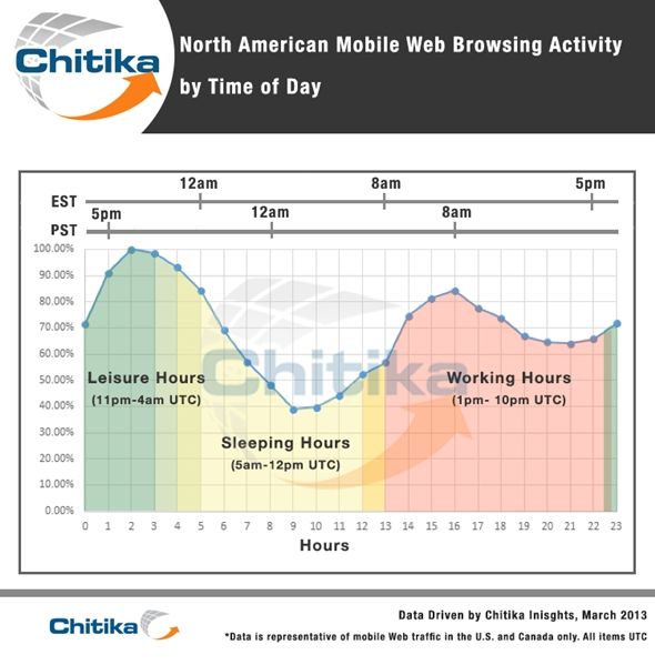
3

     t     time index, t ∈ T := {1, . . . , T }
     n     DA index, n ∈ N := {1, · · · , N }                           We assume that δb(t) has a mean of 0 and variance of δ 2 (t),
   N0      set of N 0 continuous DAs                                    and may be temporally correlated. We further assume that we
   N 00    set of N 00 = N −N 0 discrete DAs                            can make better prediction for the timeslots that are closer
   N̂t00   set of discrete DAs started earlier
                                                                        to current time, modeled by a time-dependent deviation from
   Ñt     set of DAs adjustable at time t
     b     base traffic profile, b = {b(t); t ∈ T }                     the mean, i.e., the base traffic at some future time τ ∈ T is
    pn     data rate profile of DA n, pn = {pn (t); t ∈ T }             predicted at current time t by
  pn (t)   upper bounds of DA n on the data rate at time t
    rn     constant bit rate for DA n ∈ N 00                                             bt (τ ) = b̄(τ ) + δbt (τ ),                (1)
    ln     number of timeslots to finish transmission for DA n ∈ N 00
     q     virtual deferrable traffic profile
                                                                        where the subscript t represents the timeslot when the pre-
     d     average traffic profile                                      diction is made, and δbt (τ ) has a decreasing variance δt2 (τ )
     dˆ    average traffic profile of online ODS                        as t approaches τ . More concrete model for prediction will
    dˆ∗    average traffic profile of online relaxed ODS                be introduced in Section VI. The parameters b̄ and δt will be
    d∗     average traffic profile of offline relaxed ODS
   Pn
                                                        P
           total traffic required from DA n, Pn = t∈T pn (t)            specified exogenously, and can be estimated from the historical
  Pn (t)   remaining traffic to be served for DA n ∈ Nt0                traffic records.
   xkn     change in traffic profile of DA n, xkn = pk+1  n   − pkn
    tan    arrival time of DA n
    tdn    deadline of DA n                                             B. Deferrable Applications
   An      number of feasible profiles of DA n ∈ N 00
  fn,a     a-th feasible profile of DA n ∈ N 00
                                                                           Assume that there are N DAs in the network, indexed
  un,a     probability corresponding to fn,a                            by n ∈ N = {1, · · · , N }. Each DA n is characterized by
   Fn      set of all feasible traffic profiles for discrete DAs,       an arrival time tan when it is requested or after which it
           Fn = {fn,a ; 1 ≤ a ≤ An }
   V (d)   objective value: (time) variance of d
                                                                        can be started, a deadline tdn by which its transmission must
                                                                        be done, and certain requirement or constraint on data rate
                   TABLE II: Main notation.                             pn = {pn (t); t ∈ P T }. Let Pn denote the total traffic required
                                                                        by DA n, i.e.,        t∈T pn (t) = Pn . We can classify DAs
wireless service provider shows its effectiveness in shaping the        into two main categories: continuous-rate interruptible DAs
traffic profile [24]. Also refer to [34] for a review of pricing        (or continuous DAs for simplicity) that allow any data rates
strategies.                                                             between certain upper and lower bounds and can be interrupted
                                                                        and resumed at any time before the deadline, and discrete-
    III. S YSTEM M ODEL AND P ROBLEM F ORMULATION                       rate non-interruptible DAs (or discrete DAs for simplicity)
   Consider a cellular network that serves users for different          that require certain (roughly) constant data rate and cannot
applications such as web browsing, file sharing, real-time              be interrupted once they are started. For example, system
entertainment, etc. The applications can be broadly divided             backup is usually interruptible and allows any continuous data
into two categories: deferrable applications (DAs) and non-             rates, while video conference is usually preferred to be non-
deferrable applications (non-DAs). DAs refer to those applica-          interruptible and runs at a constant (thus discrete) data rate
tions that are flexible in the starting time and/or data rate, while    once it is started.
the non-DAs refer to those that should be served immediately               Among the total N DAs, we assume there are N 0 continuous
and often have stringent data rate requirement. Please refer            DAs, indexed by n ∈ N 0 = {1, · · · , N 0 }. For each continuous
to the third paragraph of Section I and TABLE I for more                DA, denote by pn (t) and pn (t) the lower and upper bounds
detailed description and examples of DAs and non-DAs.                   on its data rate at time t ∈ T , i.e.,
   This work aims to schedule the traffic of DAs so as to flatten                    pn (t) ≤ pn (t) ≤ pn (t), t ∈ T .               (2)
the aggregate traffic profile over a day, subject to the time
                                                                        Naturally, 0 ≤ pn (t) ≤ pn (t). The lower bounds pn (t) are
constraints and rate constraints of each application. We use a
                                                                        usually zero, and the upper bounds pn (t) can be set according
discrete-time model where one day is divided equally into T
                                                                        to, e.g., the available bandwidth. The arrival time tan and the
timeslots, indexed by t ∈ T = {1, 2, · · · , T }. The duration of
                                                                        deadline tdn can be integrated into the rate constraints (2) by
a timeslot can be, e.g., 30 minutes or 1 hour [18], depending
                                                                        setting pn (t) = 0 for t < tan and t > tdn , i.e., no traffic is
on the time resolution of scheduling decisions.
                                                                        transmitted before arrival time or after deadline.
                                                                           Index the rest N 00 = N −N 0 discrete DAs by n ∈ N 00 =
A. Non-Deferrable Applications                                          {N 0 + 1, · · · , N }. For a discrete DA such as a streaming
   Non-DAs include web browsing, online gaming, and real-               application, a constant bit rate rn corresponds to a certain
time chatting with multimedia, etc. The latency tolerated by            graphic quality, e.g., rn = 3 Mbps for a SD quality movie
these applications usually varies from hundreds of millisec-            on Netflix [4], and rn = 1.2 Mbps for a HD video call on
onds to seconds. Since these applications should be served              Skype [3]. As the graphic quality usually (preferrably) does
immediately upon request, their traffic is inelastic and consti-        not change during those applications, this seemingly over-
tutes the base traffic whose profile cannot be shaped. Denote           simplified assumption of a single discrete rate is reasonable.
the base traffic profile by b = {b(t); t ∈ T }. As we can only             For each DA n ∈ N 00 with its total traffic Pn and the rate
predict the base traffic to a certain accuracy, we model it as          rn , it takes ln = Pn /rn consecutive timeslots (or equivalently
a random vector with mean b̄ = {b̄(t); t ∈ T } and random               the other way around, i.e., we calculate Pn = ln ∗ rn based
derivation δb = {δb(t); t ∈ T } from the mean, i.e., b = b̄+δb.         on ln and rn ). Therefore, the number of its feasible traffic
4
profiles is An = tdn − tan − ln + 1, wherein the a-th feasible constraint (3e). Consider the convex hull of Fn , defined as
profile is denoted as n An
X
n rn , if tan + a − 1 ≤ t ≤ tan + a + ln o conv(Fn ) := pn | pn = un,a · fn,a , ua,n ≥ 0
fn,a = pn pn (t) = . a=1
0, otherwise An
X o
00 and un,a = 1 , (4)
We denote the set of all feasible traffic profiles of DA n ∈ N
by Fn = {fn,a : 1 ≤ a ≤ An }, i.e., pn ∈ Fn , ∀n ∈ N 00 . a=1
Remark 1: All the modeled traffic parameters can be rea- where un := {un,1 , . . . , un,An } is the convex combination
sonably accessed or estimated in practice. For example, infor- coefficients, and will be interpreted as probability distribution
mation regarding total required traffic Pn and video streaming in the randomized algorithm to be introduced soon. We will
rate rn is available from metadata of traffic to be transmitted, instead solve the convex relaxation of the ODS problem by
parameters like tan and tdn are specified by the users in advance replacing (3e) with the following constraint:
(and Fn can then be calculated accordingly), whereas data rate pn ∈ conv(Fn ), n ∈ N 00 . (5)
bounds pn (t) and pn (t) can be either determined by available
We call the relaxed problem (3a)–(3d)(5) the R-ODS problem.
bandwidth or designated by the users. See, e.g., [18] for an
However, a solution p∗n ∈ conv(Fn ), n ∈ N 00 to the R-ODS
example system involving similar information requirement and
problem might not be feasible for original ODS, i.e., p∗n ∈
/ Fn .
implemented with real users and service provider. 2
solution p∗n can always be written
But since by definition (4) aP
An
as the convex combination a=1 un,a fn,a we will randomly
C. Problem Formulation pick a traffic profile pn = fn,a ∈ Fn with corresponding
We aim to schedule the traffic of DAs, so as to flatten probability un,a . That said, we will design a randomized
the aggregate traffic profile as much as possible. Denote the algorithm for the offline ODS problem, based on the solution
“average” traffic profile by d = {d(t); t ∈ T } := N1 (b + to the R-ODS problem. We will integrate it into a distributed
algorithm next.
P
n∈N pn ). Traffic flattening can be achieved by minimizing
the time variance of d, formulated as the following optimal
demand shaping (ODS) problem:
ODS: 1 X 1 X 2
min V (d) = d(t) − d(τ ) (3a)
p,d T T B. Distributed Algorithm
t∈T τ ∈T
1 X
s.t. d(t) = b(t) + pn (t) , t ∈ T , (3b)
N
n∈N Solving the R-ODS problem (and the offline ODS problem)
pn (t) ≤ pn (t) ≤ pn (t), t ∈ T , n ∈ N 0 , (3c) directly in a centralized way requires collecting information on
X
pn (t) = Pn , n ∈ N 0 , (3d) all DAs, which may incur too much communication overhead
t∈T and is impractical in the real network. Moreover, the users may
pn ∈ Fn , n ∈ N 00 . (3e) not be willing to reveal information on DAs due to privacy
Notice that the constraints (3e) for discrete DAs are non- concern. Therefore, we seek to solve it in a distributed way.
convex. In next section, we will investigate an offline algorithm Noticing that R-ODS problem has decoupled constraints, we
together with a randomized scheme for solving the ODS attempt to design an iterative and distributed algorithm based
problem under the assumption of complete information on the on the decent method [11].
base traffic and DAs. Then in Section V, we will study an Before deriving the algorithm, we establish the following
online algorithm for demand shaping under a more realistic useful results. At k-th iteration, let pk = k
P{pn ; nk ∈ N } be the
k 1
setting of incomplete information where we can only predict traffic profiles of all DAs, d = N (b + n∈N pn ) the average
the future traffic to a certain degree of accuracy. The offline traffic profile, and xkn = pk+1
n − pkn , n ∈ N the change in
ODS problem and algorithm will later serve as a benchmark traffic profile of DA n from iteration k to k + 1. We have:
to characterize the performance of the online algorithm. X k 2 X X 2
E xn 2 = V ar(xkn ) + E[xkn ] 2 , (6)
n∈N n∈N n∈N
IV. O FFLINE D EMAND S HAPING A LGORITHM where the variance V ar(xkn )
:= E
kxn k2 − kE[xkn ]k22 ,
k 2
and
1
In this section, we assume complete traffic information, i.e., E[·] denotes the average. By Jensen’s inequality,
the base traffic and arrival of DAs are accurately known, and k
X
E[xkn ]k22 ≤ N
X 2
E[xkn ] 2 . (7)
study how to solve the resulting offline ODS problem. The n∈N n∈N
offline problem and algorithm will provide insights into the Therefore, one has
online algorithm design for a realistic setting of incomplete X k 2 X X 2
information that will be considered in Section V. E k xn k2 ≤ V ar(xkn ) + N E[xkn ] 2
. (8)
n∈N n∈N n∈N
A. Convex Relaxation and Randomized Scheme
The offline ODS problem is non-convex, as each discrete 1 Notice that we consider a randomized scheme only for discrete DAs. That
DA has to pick a traffic profile from a discrete set; see said, for continuousDAs there is no randomness and their variance is zero.5
And it follows that algorithm is not only preserving privacy of the users, but also
2
T N E[V (d k+1 k
)|p ] − V (d )
k scalable and thus capable of quick response, which is crucial
X k 2 X especially in real-time implementation in Section V.
xn k2 + 2hN dk , xkn i
= E k
The computational complexity of the Off-DS algorithm is
X n∈N X n∈N X estimated as follows for completeness. Given certain accuracy
≤ V ar(xkn ) + N kE[xkn ]k22 + 2 E[hN dk , xkn i]
requirement > 0 in the objective function value, the
n∈N n∈N n∈N
X descent method requires O(log(1/)) iterations [11]. At each
X
= 2hN dk , xkn i + N kxkn k22 + 2hN dk , E[xkn ]i iteration, DAs solves an easy quadratic programming with a
n∈N 0
n∈N 00 polynomial complexity of O(T O(1) ) [33]. On the other hand,
+ N kE[xkn ]k22 + V ar(xkn ) . (9) the coordinator calculates the average traffic profile which
Denote by W1 the first term in (9) and W2 the second. For requires O(N ) complexity each iteration. As a result, the Off-
n ∈ N 0 , we choose pk+1 so as to minimize W1 , i.e., to solve DS algorithm requires overall computational complexity of
n
O (N + T O(1) ) log(1/) .
min 2hdk , pn − pkn i + kpn − pkn k22 (10a)
pn Remark 2: For simpler expression, we use pn as the deci-
s.t. (3c) − (3d). (10b) sion variable for DA n ∈ N 00 in algorithm design and analysis,
On the other hand, after some mathematical manipulations, while in real implementation, it is more convenient to use
we have probability distribution un as the equivalent decision variable.
X Also notice that, if there is no continuous DA, Algorithm 1
2N hdk − pkn , E[pk+1 k+1 2
k
W2 = n ]i+(N −1)kE[pn ]k2 +Π , reduces to the stochastic algorithm in [14]. We expect that
n∈N 00
the solution approach—randomized algorithm based on the
where Π is a constant given pkn . For n ∈ N 00 , we choose
k
“steepest” descent method for the convex relaxed problem—
pn∗k+1 so as to minimize W2 , i.e., to solve that we lay out in Sections IV-A and IV-B will find broad
N −1 application in designing efficient algorithms for optimization
min 2hdk − pkn , pn i + kpn k22 . (11)
pn ∈conv(Fn ) N problems that involve both continuous and discrete decision
In essence, what we have done is to maximize the expected variables. 2
incremental decrease in the objective value V (d) at each
iteration (i.e., steepest descent). This motivates a distributed
demand shaping algorithm with the collaboration of a coor-
dinator; see Algorithm 1. The wireless service provider can
implement a logical coordinator at the base station. C. Convergence
Algorithm 1 Offline Demand Shaping (Off-DS) Algorithm Before showing the convergence of the Off-DS algorithm,
we first establish two useful relations. For each DA n ∈ N 0 ,
At k-th iteration:
since pk+1
n solves the problem (10), we have the first-order
1) Upon gathering traffic profiles pkn from DAs, the coordi- optimality condition
nator calculates the average traffic profile dk = N1 (b +
P k hpk+1 − pkn + dk , pn − pk+1
n i≥0 (12)
n∈N pn ) and announces it to DAs (or the end users)
n
over a signaling or control channel. for any feasible pn . Set pn = pkn to obtain
2) Upon receiving the average traffic profile dk , hd k
, pk+1 − pkn i ≤ −kpk+1 − pkn k22 . (13)
0 n n
• DA n ∈ N updates its traffic profile by 00
2
For each DA n ∈ N , recalling that = p∗k+1
n E[pk+1
n ], by the
pk+1
n = arg min pn − pkn + dk 2 first-oder optimality condition, we have
pn
s.t. (3c)–(3d), N
h (dk − pkn ) + p∗k+1
n , pn − p∗k+1
n i≥0 (14)
and submits it to the coordinator. N −1
• DA n ∈ N 00 calculates the average traffic profile by for any feasible pn . Set pn = pkn to get
N 2 hN dk , p∗k+1
n − pkn i ≤ −(N − 1)kp∗k+1n − pkn k22
pn∗k+1 = arg min pn − (pkn − dk ) ,
pn ∈conv(Fn ) N −1 2 + hpkn , p∗k+1
n − pkn i. (15)
∗k+1
PAn k+1
which is pn = a=1 un,a fn,a , and then ran- Now, construct a filtration Σ∗ of the probability space
domly chooses a traffic profile pk+1 n = fn,a with {Ω, Σ, P}, where the sample space Ω is the feasible set
probability uk+1
n,a and submits it to the coordinator. specified by the constraints (3c)–(3e), the σ-algebra Σk =
Ω, k ≥ 0, and P(Σk ) = {δ(pn − pkn ), n ∈ N 0 ; ukn,a , 1 ≤
a ≤ An , n ∈ N 00 }, i.e., determined by the k-th iteration of
The Off-DS algorithm is a distributed algorithm wherein
the Off-DS algorithm.
each DA solves its own simple optimization problem based on
its previous decision, the average traffic profile dk , and local Theorem 1: The pair (V (d), Σ∗ ) is a supermartingale. 2
constraints, while the coordinator collects the proposed traffic Proof: First, notice that V (d) is bounded from below. So,
profiles and updates the average traffic profile. Therefore, this E[− min{0, V (d)}] < ∞. Second, applying relations (13)–6
(15) to equation (9), we obtain discrete DAs increases, i.e.,
2 k+1 k k
lim Goff
T N E[V (d )|p ] − V (d ) r = 0. (18)
N 00 →∞
2
X X
k 2
≤ −N kxn k2 + V ar(xkn ) P
n∈N 0 n∈N 00 Proof: For notational simplicity, let cd := t∈T d(t)/T ,
2
+ 2hpkn , pn∗k+1 − pkn i
E[xkn ] 2
+ (−N + 2) which is a constant given the total amount of traffic. The
X X 2 objective value can be written as
= −N kxkn k22 + (−N + 1) E[xkn ] 2
1 1
n∈N 0 n∈N 00 V (d) = kd − cd · 1k22 = (kdk22 + c2d k1k22 − 2hd, 1i)
≤ 0, T T
1
i.e., E[V (dk+1 )|pk ] ≤ V (dk ). By definition, (V (d), Σ∗ ) is a = (kdk22 + T · c2d − 2T · cd ),
T
supermartingale [16].
where only the part kdk22 contains decision variables. We can
Notice that (V (d), Σ∗ ) is a nonnegative supermartingale.
thus write the gap Goff as
By the martingale convergence theorem [16], the following
1
Goff = V (d∞ ) − V (d∗ ) = kd∞ k22 − kd∗ k22
result is immediate.
T
Corollary 1: V (d∞ ) = limk→∞ V (dk ) exists almost =
1
− kd∞ − d∗ k22 + h2d∞ , d∞ − d∗ i
surely, where V (d∞ ) is some random variable. 2 T
Theorem 2: Denote by P ∞ an “equilibrium” distribution 1
≤ h2d∞ , d∞ − d∗ i
over traffic profiles that (V (d), Σ∗ ) converges to. The support T X
2 ∞ ∞ ∗
X
∞ ∞ ∗
of P ∞ is a singleton. 2 = hN d , p n − pn i + hN d , p n − p n i
N2
Proof: When (V (d), Σ∗ ) converges, E[V (dk+1 )|pk ] = n∈N 0
2 X ∞ ∞
n∈N 00
∗
V (dk ). This requires E[xkn ] = E[xkn0 ], n, n0 ∈ N , pk+1 n = ≤ hpn , pn − pn i
TN2
pkn , n ∈ N 0 , and pn∗k+1 = pkn , n ∈ N 00 for (8), (13), and n∈N 00
2 X
(15) to hold with equality. Notice that p∗k+1n = pkn implies ≤ kp∞ 2
n k2 ,
pn = pn , as different feasible traffic profiles of DA n ∈ N 00
k+1 k TN2 00
n∈N
are linearly independent. Thus, pk+1 n = pkn , n ∈ N . So, the where the second inequality follows from (16). Note that
∞
support of P contains only one point. kp∞ 2 00
n k2 is a constant for n ∈ N . Then the relative gap Gr
off
Denote by p∞ an “equilibrium” traffic profile of the Off-DS can be bounded as
algorithm, i.e., if pk = p∞ , then pk+1 = p∞ . Obviously the 2 X
Goff
r ≤ kp∞ 2 ∗
n k2 /V (d )
set of equilibrium profiles is not empty, as an optimum of the TN2 00
n∈N
offline ODS problem is an equilibrium. The following result ∞ 2
P
n∈N 00 kpn k2
follows immediately from Theorem 2 and Corollary 1. = ,(19)
kb + n∈N p∗n k22 + N 2 (T · c2d − 2T · cd )
P
Theorem 3: The Off-DS algorithm converges almost surely
whose numerator increases linearly with N 00 and denominator
to an equilibrium traffic profile. 2
increases linearly with the square of N 00 . Equation (18)
By equations (12)–(14), we have the following optimality
follows.
conditions at equilibrium p∞ : for any feasible pn ,
X Remark 3: We use the relaxed problem R-ODS for compar-
hb + p∞ ∞
m , pn − pn i ≥ 0, n ∈ N ,
0
(16a) ison instead of the ODS problem for two reasons. First, it is
m∈N
X difficult to characterize the optimum of the non-convex ODS
hb + p∞ ∞
m , pn − pn i ≥ 0, n ∈ N .
00
(16b) problem, and thus evaluating the gap between the equilibrium
m6=n of the Off-DS algorithm and the optimum of ODS problem is
mathematically hard. Second, R-ODS achieves an optimal ob-
jective value that is not greater than ODS, resulted from convex
D. Performance Analysis of the Offline Algorithm relaxation for the discrete decision variables. Therefore, Goff
We now characterize the performance of Off-DS algorithm provides an upper bound for the “actual” sub-optimality, i.e.,
with respect to the relaxed problem R-ODS that at optimum the gap between the equilibrium of Off-DS and the optimum
may attain a lower objective value than the ODS problem. of ODS. 2
Specifically, denote by p∗ the solution of R-ODS, we bound
the gap between the equilibrium of the Off-DS algorithm and V. O NLINE D EMAND S HAPING A LGORITHM
the solution of the R-ODS P problem as: Goff := V (d∞ ) −
∗ ∞ ∞ ∗ In this section, we consider a realistic setting with incom-
V (d ), where d = (b + n∈N pn )/N and d = (b +
∗ ∞ ∗ plete information where we can only predict future traffic
off
))/V (d∗ )
P
n∈N n p )/N . Denote by Gr := (V (d ) − V (d
to a certain degree of accuracy, and study online demand
the relative gap achieved by the Off-DS algorithm.
shaping that makes decisions based on the prediction of future
Theorem 4: For the Off-DS algorithm, the gap Goff is
traffic and updates the decision as new information becomes
bounded as follows:
2 X available.
Goff ≤ kp∞ 2
n k2 . (17) A typical algorithm used in this setting is the receding
TN2 00
n∈N horizon control; see, e.g., [25]. However, as the objective
Moreover, the relative gap diminishes as the number N 00 of function (3a) does not have a nice additive structure, receding7
horizon control algorithm does not admit an easy analysis. Algorithm 2 Online Demand Shaping (On-DS) Algorithm
We will instead extend a shrinking horizon control algorithm, At each timeslot t ∈ T :
(t−1)
which is used in [15] that studies mathematically the same 1) Denote by pn , n ∈ Nt−1 the schedules determined
problem with only continuous DAs, to include discrete DAs, by time t − 1, and by N̂t00 ⊆ Nt00 the set of discrete
and apply it to our online demand shaping (online DS) DAs that has been started before time t. For each DA
problem. n ∈ N̂t00 , set its schedule pn (t; T ) = {pn (τ ); t ≤ τ ≤ T }
(t−1)
as pn (τ ) = pn (τ ), t ≤ τ ≤ T .
A. Online Algorithm 2) Solve the ODSt problem iteratively: at k-th iteration,
We assume that the number mt of DAs arriving at time t a) Upon gathering traffic profiles pkn (t : T ) = {pkn (τ ); t ≤
is randomly distributed with a mean λt and variance (δλt )2 , τ ≤ T } from DAs n ∈ Ñt , the coordinator solves
and the total amount of traffic of each DA is randomly XT X X 2
distributed with a mean P and variance (δP )2 . Denote by min bt (τ ) + q(τ ) + pn (τ ) + pkn (τ )
q(t+1:T )
Nt0 = {1, · · · , Nt0 } the set of continuous DAs and Nt00 = τ =t+1 n∈N̂t00 n∈Ñt
{N 0 + 1, · · · , Nt } the set of discrete DAs that have arrived s.t. (20f),
by time t ∈ T , and let Nt = Nt0 ∪ Nt00 and Nt00 = Nt − Nt0 . to obtain a virtual deferrable traffic {q k (τ ); t + 1 ≤
k
Notice that we cannot reschedule the remaining traffic of a τ ≤ T }, and then calculates P traffickd (τ) =
the average
discrete DA that has already started. Denote by Ñt00 ⊆ Nt00 1 k
P
Nt bt (τ )+q (τ )+ p
n∈N̂t00 n (τ )+ n∈Ñt n ) for
p (τ
the set of discrete DAs that have not been started by time t. τ ≥ t and announces it to DA n ∈ Ñt over a signaling
For DA n ∈ Ñt00 , denote by Fn (t) = {fn,a ; 1 ≤ a ≤ An (t)} or control channel.
the set of feasible traffic profiles at time t. Let Ñt = Nt0 ∪ Ñt00 b) Upon receiving the average traffic profile dk ,
be the set of DAs whose profiles are still adjustable at time t 0 k+1
• DA n ∈ Nt obtains pn (t : T ) by
(i.e., all the continuous DAs and the discrete DAs that have 2
not started by time t). min pn (t : T ) − pkn (t : T ) + dk (t : T ) 2
pn (t:T )
At time t, we make a prediction bt (t : T ) of base traffic for s.t. (20c)–(20d),
the rest timeslots of the day, and we also have the information and submits the updated profile to the coordinator.
on DAPn ∈ Nt and the expected total future deferrable • DA n ∈ Ñt00 calculates p∗k+1 (t : T ) by
T n
traffic τ =t+1 P λτ . Following [15], we introduce a virtual 2
Nt
deferrable trafficPprofile q(t : TP ) = {q(τ ); t ≤ τ ≤ T } with min pn (t : T ) − (pkn (t : T ) − dk (t : T ))
q(t) = 0 and
T
q(τ ) =
T pn (t:T ) Nt − 1 2
τ =t τ =t+1 P λτ , to emulate the s.t. pn (t : T ) ∈ conv(Fn (t)), n ∈ Ñt00 ,
impact of the future deferrable traffic upon the current demand
shaping decision. With the afore setup, we aim to schedule and represents it as a convex combination p∗k+1
n =
PAn (t) k+1
reschedule the DAs, so as to solve the following problem at a=1 u f
n,a n,a , and randomly chooses a traffic
each timeslot t ∈ T . profile pk+1
n = fn,a with probability uk+1
n,a and
ODSt : submits it to the coordinator.
T PT
1 X d(s) 2
min V (d) = d(τ ) − s=t (20a)
T −t+1 τ =t T −t+1 B. Performance Analysis of the Online Algorithm
over p(t : T ), d(t : T ), q(t : T ) We now characterize the performance of On-DS algorithm
P
bt (τ )+q(τ )+ n∈Nt pn (τ ) with respect to the result of Off-DS algorithm which serves
s.t. d(τ ) = , τ ≥ t, (20b)
Nt as a benchmark. We will make the following assumptions to
pn (τ ) ≤ pn (τ ) ≤ pn (τ ), τ ≥ t, n ∈ Nt0 , (20c) simplify the analysis and obtain insights into how uncertainties
T
X affect the performance of On-DS algorithm.
pn (τ ) = Pn (t), n ∈ Nt0 , (20d) Assumption 1: The amount of deferrable traffic is large and
τ =t flexible enough so that a valley-filling schedule exists at every
pn ∈ Fn (t), n ∈ Ñt00 , (20e) time t = 1, . . . , T , i.e., there exists some constant C(t) ≥
T T
X X bt (τ ), ∀τ = t, . . . , T such that
q(τ ) = P λτ , (20f)
τ =t τ =t+1 N d(t) = C(t)
T T Nt
where p(t : T ) = {pn (τ ); t ≤ τ ≤ T, nP∈ Ñt }, d(t : T ) = 1 X X X
= bt (τ ) + P λτ + Pn (t) . (21)
t−1
{d(τ ); t ≤ τ ≤ T }, and Pn (t) = Pn − τ =1 pn (τ ), n ∈ Nt0 T − t + 1 τ =t τ =t+1 n=1
is the amount of traffic to be served at or after time t. 2
We can solve the ODSt problem at each timeslot the same Remark 4: Assumption 1 looks a strong assumption, and
way as we solve the offline ODS problem (3), constituting an we do not have empirical evidence to support it as demand
online demand shaping algorithm; see Algorithm 2, wherein shaping has not being widely adopted in current cellular
the convergence (and computational complexity) of Step networks. However, with increasing penetration of deferrable
2) can be established (and analyzed) in the same way as traffics and users, this assumption expects to hold. One purpose
Algorithm 1. of algorithm design as in this paper and incentive design8
rem 4, we have
ˆ − V (dˆ∗ ) ≤ 2 X
kp̂n k22 ,
0 ≤ E V (d) (25)
TN2
n∈N 00
2 X
kp̂n k2 ≤ E V (d ) − V (d∞ ) ≤ 0.
2 ∗
− (26)
TN2
n∈N 00
For the second term of (23), under Assumptions 1–2, following
[15], we get
T T −1
Fig. 2: Strategy to calculate the gap between the equilibrium (δλ)2 X 1 δ2 X 2 T − t − 1
E V (dˆ∗ )−V (d∗ ) =
of the On-DS algorithm and that of Off-DS algorithm. + 2 F (t) .
T t=2 t T t=0 t+1
(27)
Combine (25)–(27) to obtain (24).
as in [18] is to facilitate and incentivize wide adoption of
Theorem 5 indicates that, the size of the gap between online
demand shaping. On the other hand, valley-filling represents
and offline algorithms changes monotonically with prediction
the scenario where demand shaping is most useful and presents
error of both base traffic and future arrival of deferrable traffic.
a benchmark for the potential of demand shaping. Mathe-
Accordingly we can improve the result of On-DS algorithm
matically, it is very difficult to analyze the performance of
by implementing better prediction mechanism, e.g., On-DS
the online algorithm under more general assumption than
algorithm which updates its prediction to keep the value of
Assumption 1. However, notice that in numerical examples in
prediction error small. Also, if the impulse response f is
Section VI, we do not impose Assumption 1 while the results
chosen to fade quickly enough, then as we have finer time
still fall into the bound specified in Theorem 5. 2
granularity, we have T → ∞, and Gon → 0, which intuitively
Assumption 2: The base traffic prediction at t is modeled indicates that, with infinitely small timeslot, we can update
as the following causal filter our decisions frequently enough to mitigate prediction errors,
T
X and therefore have a negligible performance gap.
bt (τ ) = b̄(τ ) + e(s)f (τ − s), τ = 1, . . . , T, (22) Lastly, similar to Theorem 4, define a relative gap Gon r :=
s=1
G /V (d∞ ). The following result is immediate.
on
where e = {e(s)}Ts=1 is an uncorrelated sequence of indepen- Theorem 6: The relative gap Gon r diminishes as the number
dent and identically distributed random variables with mean of discrete DAs N 00 increases, i.e.,
0 and variance δ 2 , and f = {f (τ )}∞ τ =−∞ is the impulse
t lim Gon
r = 0. (28)
2
P
response with f (0) = 1. Let F (t) := s=0 f (s). N 00 →∞
We denote by Gon the gap defined as the expected difference 2
Remark 5: It is worth noting that equation (28) does not
between the results of On-DS algorithm and Off-DS algo-
ˆ − V (d∞ )], where E denotes the necessarily imply a monotone decreasing of Gon r with respect
rithm, i.e., Gon = E[V (d)
ˆ ∞ to N 00 . This can be seen from Fig. 6 in Section VI that does
expectation, and d and d denote the average traffic profiles
not show a decreasing Gon 00
r as N increases. 2
achieved by the On-DS algorithm and the offline-DS algorithm
By equations (25) and (27), it is straightforward to obtain
respectively. It turns out that direct calculation of this gap is
the following result.
difficult. We therefore utilize two intermediate variables: d∗ ,
Corollary 2: The expected difference between the On-DS
the average traffic profile achieved by the R-ODS problem,
algorithm and the optimum of the R-ODS problem is bounded
and dˆ∗ , the average traffic profile achieved by the relaxed
as follows:
online DS, i.e., the counterpart of R-ODS problem in the
ˆ − V (d∗ )] ≤ 2
X
online scenario. Similar notations are applied to individual E[V (d) kp̂n k22
TN2
traffic profile pn . With the relation shown in Fig. 2, we can T
n∈N 00
T −1
write online gap as (δλ)2 X 1 δ2 X 2 T − t − 1
+ + 2 F (t) .
Gon = E V (d)−V
ˆ (dˆ∗ )+V (dˆ∗ )−V (d∗ )+V (d∗ )−V (d∞ )
T t=2 t T t=0 t+1
ˆ − V (dˆ∗ ) + E V (dˆ∗ ) − V (d∗ )
2
= E V (d)
+ E V (d∗ ) − V (d∞ ) .
(23) VI. N UMERICAL E XAMPLES
Theorem 5: The gap, i.e., the expected difference between In this section, we provide numerical examples to evaluate
the results of On-DS algorithm and Off-DS algorithm is the performance of the On-DS algorithm. We use certain
bounded as follows: composite traffic traces to drive simulations to show the impact
of base traffic prediction errors, deferrable traffic prediction
ˆ − V (d∞ )] ≤ 2
X
Gon = E[V (d) kp̂n k22 errors, and deferrable traffic penetration levels. We expect the
TN2 00
n∈N conclusions obtained to hold for real traffic.
T T −1
(δλ)2 X 1 δ2 X 2 T − t − 1
+ + 2 F (t) . (24)
T t=2 t T t=0 t+1 A. Experimental Setup
2 Consider a 48-hour period of time starting from 4:00 pm to
Proof: Applying the approach and results from Theo- 3:59 pm two days later. We divide the 48 hours equally into9
15.13
1100
average base traffic
1000 "real" base traffic
15.125
objective function value
900
aggregate traffic
800 15.12
700
15.115
600
500 15.11
400
15.105
300 1 10 20 30 40
16:00 22:00 04:00 10:00 16:00
time of day number of iterations
Fig. 4: Repetitive experiments show that a number of 20 to
Fig. 3: Base traffic: the average (blue/dotted) and a “real” trace 30 iterations give a satisfying result in terms of convergence.
(red/solid).
3) Benchmarks for Comparison: We compare the perfor-
96 timeslots, each 30 minutes long. We consider scheduling mance of the On-DS algorithm with a few typical benchmarks
traffic that arrives within the first 24 hours only, which may to evaluate the impact of base traffic prediction error, the
be allocated to the second 24 hours. benefit of updating the prediction in real time, and the impact
1) Non-deferrable Traffic: The “real” trace we use for non- of deferrable traffic’s penetration level. We thus consider the
deferrable traffic, or base traffic, is shown in Fig. 3 (red line). It followings five cases in our experiments:
is constructed by random fluctuation around the average base (0) Offline demand shaping w/ Off-DS algorithm. We use
traffic trace (blue line) composed based on North American “real” trace for future base traffic and use arrival infor-
mobile web browsing activity by time of day in 2013 [21], mation recorded from case (1) below for DAs. Applied
shown in Fig. 1. As modeled in Section III-A, the prediction with Off-DS algorithm, this case gives the optimal per-
of base traffic follows (1), consisting of average base traffic formance used as benchmark to characterize the gap of
b̄(τ ) and random deviation δbt (τ ) from the average value. other cases.
Following [15], at time t, δbt (τ ) is modeled as (1) Online demand shaping w/ On-DS algorithm. We make
τ
X prediction for both DAs’ arrival and base traffic in the
δbt (τ ) = ωs (τ ), t < τ ≤ T, (29) future. Prediction is updated at each timeslot. We run
s=t+1
On-DS algorithm to schedule traffic.
where ωs (τ ) are random variables of Gaussian distribution (2) Online demand shaping w/ exact information for base
with 0 mean and variances traffic and w/o exact information for DAs. We use “real”
σ2 trace for base traffic and prediction for DAs. We apply
E[ωs2 (τ )] = , 1 ≤ s ≤ τ ≤ T. (30)
τ −s+1 On-DS algorithm. Comparison of case (2) with case (1)
In this way, δbt (τ ) has decreasing variance as t approaches τ , shows the impact of uncertainty in base traffic.
simulating a gradually improving prediction for some future (3) Demand shaping w/ updating prediction of base traffic
timeslot τ as one gets closer to it. In simulation, we take the and w/ exact information for DAs. We use DAs arrival
values of σ 2 in (30) from 0 to 100 with increment of 10, information recorded from case (1). Instead of applying
corresponding to a root-mean-square prediction error (RMSE) virtual deferrable traffic, we schedule traffic profiles for
ranging from 0% to 32%, looking 48 timeslots (24 hours) all the future deferrable traffic. Since the exact base
ahead. traffic information is not available, we updated base
2) Deferrable Traffic: We assume that the number of DAs traffic prediction at each timeslot. Comparison of case (3)
arriving at each timeslot follows a “shifted” Poisson process and (1) shows the impact of uncertainty in DAs arrival
m + poissrnd(λp ), with m ≥ 0 and poissrnd(λp ) denoting a prediction.
Poisson process with rate λp . Here, we set λp = 4, while each (4) Demand shaping w/o updating prediction of base traffic
DA has a 50-50 chance to require continuous- or discrete-rate and w/ exact information for DAs. We use prediction of
traffic. The total traffic Pn of each DA is uniformly distributed the base traffic at the beginning (t = 1) without further
in [P , P ] where we set P = 12 and P = 24. The deadline for updating, and use arrival information recorded from case
DA n is uniformly distributed in [tan + ln + D, tan + ln + D], (1) for DAs. This case shows how the online algorithm
where ln = pPn /pn q is the minimum number of timeslots benefits from updating prediction at each timeslot.
required by the DA calculated by ceiling function p·q. We set We use the metric of relative gap Gr (d) = (V (d) −
D = 6, D = 14, and a universal bit rate upper bound pn = 3. V (d0 ))/V (d0 ) to evaluate the performance, where d0 is the10
2
Fig. 5: Base traffic prediction error has little impact on online Fig. 6: Increasing penetration level of deferrable traffic does
algorithms with updated base traffic prediction. not influence the relative gap of online algorithms.
results obtained from case (0). Also notice that when d is cal- VII. C ONCLUSION
culated based on case (1), Gr (d) becomes Gon r in Theorem 6. We have formulated demand shaping in cellular networks
as an optimization problem that minimizes the time variation
in aggregate traffic subject to the rate and time requirements
B. Experiment Results of the applications. We design a distributed and randomized
Considering randomness in DAs’ arrivals, base traffic pre- offline demand shaping algorithm under complete traffic in-
diction, and deciding traffic profiles for discrete DAs, we run formation and prove its almost surely convergence. We then
simulation for 10 times, and take the average as the final result consider a realistic setting with incomplete information where
to present. we can only predict future traffic to a certain degree of
1) Convergence Speed: We first run a case of randomly accuracy, and design an online demand shaping algorithm
generated 143 continuous DAs and 150 discrete DAs by Off- that updates the schedules of deferrable applications each
DS algorithm with different numbers of iterations ranging time new information is available, based on solving at each
from 1 to 40 for 10 times. Because of the random process timeslot an optimization problem over a shrinking horizon
in choosing traffic profiles for discrete DAs, we observe from the current time to the end of the day. We compare
oscillation in objective function values for each individual the performance of the online algorithm against the optimal
run. However, the oscillation has a trend of diminishing as offline algorithm analytically and numerically. As future work,
the more iterations are implemented, with satisfying enough we are investigating to integrate the incentive mechanisms
results generated from running 20 to 30 iterations. See Fig.4 such as the smart data pricing into the demand shaping
for the results. We will implement a number of 30 iterations algorithm design. We also plan to develop a platform to enable
to make each decision for the rest of simulation. automatic demand shaping in cellular networks and investigate
2) Impact of Base Traffic Prediction Error: As described the related practical issues.
in Section VI-A, we can tune the variance σ 2 to emulate
situations with different prediction errors in base traffic. As ACKNOWLEDGEMENT
Fig. 5 shows, with updated prediction, case (1)’s performance We would like to thank Seungil You for help with simula-
is barely affected by the increasing prediction error, keeping its tions and Lingwen Gan for careful comments.
relative gap under 5%. This is almost as good as that of case
(2) with perfect base traffic information. We can also see from R EFERENCES
the performance of case (3) the pure impact from prediction
[1] Airtel launches unlimited-usage night plans for calls, internet.
errors, while case (4) gives an example showing what happens http://businesstoday.intoday.in/story/airtel-night-plans-unlimited-usage
if there is no updated prediction. -for-calls-internet/1/205272.html.
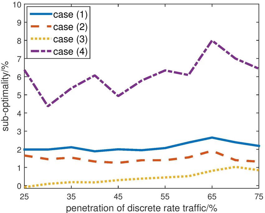
3) Impact of Penetration Level of Discrete DAs: In this [2] AT&T still throttles “unlimited data”—even when network not con-
gested. https://arstechnica.com/information-technology/2014/12/att-still
case, we fix the prediction error in base traffic at σ 2 = 40 and -throttles-unlimited-data-even-when-network-not-congested/.
the average number of DAs’ arrival at each timeslot at λp = 4. [3] How much bandwidth does Skype need? https://support.skype.com/en/f
We then tune the penetration level of discrete DAs from 25% aq/FA1417/how-much-bandwidth-does-skype-need.
[4] Netflix internet connection speed recommendations. https://help.netflix.
to 75% with granularity of 5%. As shown in Fig. 6, the relative com/en/node/306.
gap maintains relatively unaffected by the changes of discrete [5] Sprint night and weekend minutes. http://shop2.sprint.com/en/stores/p
DAs whose penetration has increased by three times. Here, we opups/voice nights weekends 7pm popup.shtml.
[6] T-mobile now throttling mobile hotspots when network is con-
do not observe a decreasing relative gap mainly because the gested. https://arstechnica.com/information-technology/2016/10/t-mobil
gap is not monotonically decreasing with number of N 00 . e-now-throttling-mobile-hotspots-when-network-is-congested/.11
[7] Telkom night surfer plan. http://www.telkommobile.co.za/plans/prepaid [33] F. A. Potra and S. J. Wright. Interior-point methods. Journal of
-data/60gbpromo/. Computational and Applied Mathematics, 124(1):281–302, 2000.
[8] Verizon nationwide for business plans. http://business.verizonwireless.c [34] S. Sen, C. Joe-Wong, S. Ha, and M. Chiang. Pricing data: A look
om/content/b2b/en/shop-business-products/business-plans/nationwide-f at past proposals, current plans, and future trends. arXiv preprint
or-business.html. arXiv:1201.4197, 2012.
[9] Verizon wireless to slow down users with unlimited 4G LTE [35] S. Sen, C. Joe-Wong, S. Ha, and M. Chiang. Smart data pricing (SDP):
plans. https://arstechnica.com/information-technology/2014/07/verizo Economic solutions to network congestion. SIGCOMM eBook on Recent
n-wireless-to-slow-down-users-with-unlimited-4g-lte-plans/. Advances in Networking, 2013.
[10] A. Balasubramanian, R. Mahajan, and A. Venkataramani. Augmenting [36] J. Tadrous, A. Eryilmaz, and H. El Gamal. Proactive resource allocation:
mobile 3G using WiFi. Proceedings of International Conference on Harnessing the diversity and multicast gains. IEEE Transactions on
Mobile Systems, Applications, and Services, pages 209–222, 2010. Information Theory, 59(8):4833–4854, 2013.
[11] S. Boyd and L. Vandenberghe. Convex Optimization. Cambridge [37] L. Zhang. Smart Data Pricing in Wireless Data Networks: An Economic
University Press, 2004. Solution to Congestion. PhD thesis, The Hong Kong Polytechnic
[12] L. Chen, L. Jiang, N. Li, and S. H. Low. Optimal demand response: University, 2016.
Problem formulation and deterministic case. Control and Optimization [38] S. Zhao, X. Lin, and M. Chen. Peak-minimizing online EV charging:
Theory for Electric Smart Grids, 2012. Price-of-uncertainty and algorithm robustification. Proceedings of IEEE
[13] M. H. Cheung, F. Hou, J. Huang, and R. Southwell. Congestion-aware Conference on Computer Communications (INFOCOM), pages 2335–
distributed network selection for integrated cellular and Wi-Fi networks. 2343, 2015.
IEEE Journal on Selected Areas in Communications, 35(6):1269 –1281, [39] X. Zhou and L. Chen. Demand shaping in cellular networks. Proceed-
2017. ings of Annual Allerton Conference on Communication, Control, and
[14] L. Gan, U. Topcu, and S. H. Low. Stochastic distributed protocol for Computing (Allerton), pages 621–628, 2014.
electric vehicle charging with discrete charging rate. Proceedings of [40] X. Zhou, E. Dall’Anese, L. Chen, and A. Simonetto. An incentive-based
Power and Energy Society General Meeting, pages 1–8, 2012. online optimization framework for distribution grids. IEEE Transactions
[15] L. Gan, A. Wierman, U. Topcu, N. Chen, and S. H. Low. Real- on Automatic Control, 2017.
time deferrable load control: Handling the uncertainties of renewable
generation. Proceedings of International Conference on Future Energy
Systems, pages 113–124, 2013.
[16] G. R. Grimmett and D. R. Stirzaker. Probability and Random Process.
Oxford University Press, third edition, 2001.
[17] S. Ha, S. Sen, C. Joe-Wong, Y. Im, and M. Chiang. Tube survey
questions and demographics. http://www.princeton.edu/∼cjoe/TUBE S
urvey.pdf, Jan 2012.
[18] S. Ha, S. Sen, C. Joe-Wong, Y Im, and M. Chiang. Tube: Time-
dependent pricing for mobile data. ACM SIGCOMM Computer Com-
munication Review, 42(4):247–258, 2012.
[19] M. H. Hajiesmaili, L. Deng, M. Chen, and Z. Li. Incentivizing device-to-
device load balancing for cellular networks: An online auction design.
IEEE Journal on Selected Areas in Communications, 35(2):265–279,
2017.
[20] Cisco Visual Networking Index. Global mobile data traffic forecast
update, 2016–2021. 2017.
[21] Chitika Insights. Hour-by-hour examination: Smartphone, tablet, and
desktop usage rates, 2013.
[22] G. Iosifidis, L. Gao, J. Huang, and L. Tassiulas. A double-auction
mechanism for mobile data-offloading markets. IEEE/ACM Transactions
on Networking (TON), 23(5):1634–1647, 2015.
[23] L. Jiang, S. Parekh, and J. Walrand. Time-dependent network pricing
and bandwidth trading. Proceedings of IEEE Network Operations and
Management Symposium Workshops, pages 193–200, 2008.
[24] C. Joe-Wong, S. Ha, and M. Chiang. Time-dependent broadband pricing:
Feasibility and benefits. Proceedings of International Conference on
Distributed Computing Systems (ICDCS), pages 288–298, 2011.
[25] W. H. Kwon and A.E. Pearson. A modified quadratic cost problem
and feedback stabilization of a linear system. IEEE Transactions on
Automatic Control, 22(5):838–842, Oct 1977.
[26] J. Lee, Y. Yi, S. Chong, and Y. Jin. Economics of WiFi offloading:
Trading delay for cellular capacity. IEEE Transactions on Wireless
Communications, 13(3):1540–1554, 2014.
[27] K. Lee, J. Lee, Y. Yi, I. Rhee, and S. Chong. Mobile data offloading:
How much can WiFi deliver? IEEE/ACM Transactions on Networking,
21(2):536–550, 2013.
[28] N. Li. A market mechanism for electric distribution networks. Pro-
ceedings of IEEE Annual Conference on Decision and Control (CDC),
pages 2276–2282, 2015.
[29] N. Li, L. Chen, and S. H. Low. Optimal demand response based on
utility maximization in power networks. Proceedings of IEEE Power
Engineering Society General Meeting, July 2011.
[30] F. Mehmeti and T. Spyropoulos. Is it worth to be patient? Analysis and
optimization of delayed mobile data offloading. Proceedings of IEEE
INFOCOM, pages 2364–2372, 2014.
[31] F. Parise, M. Colombino, S. Grammatico, and J. Lygeros. Mean field
constrained charging policy for large populations of plug-in electric
vehicles. Proceedings of IEEE Annual Conference on Decision and
Control (CDC), pages 5101–5106, 2014.
[32] I. C. Paschalidis and J. N. Tsitsiklis. Congestion-dependent pricing of
network services. IEEE/ACM Transactions on Networking, 8(2):171–
184, 2000.You can also read