Dialectometry-Based Classification of Central-Southern Italian Dialects
←
→
Page content transcription
If your browser does not render page correctly, please read the page content below

Dialectometry-Based Classification of
            Central-Southern Italian Dialects
                              Antonio Sciarretta
                                   July 2022

Abstract
This paper provides a new classification of Central-Southern Italian dialects us-
ing dialectometric methods. All varieties considered are analysed and cast in a
data set where homogeneous areas are evaluated according to a selected list of
phonetic features. Using numerical evaluation of these features and Manhattan
distance, a linguistic distance rule is defined. On this basis, the classification
problem is formulated as a clustering problem, and a k-means algorithm is used.
Additionally, an ad-hoc rule is set to identify transitional areas and silhouette
analysis is used to select the most appropriate number of clusters. While mean-
ingful results are obtained for each number of clusters, a nine-group classification
emerges as the most appropriate. As the results suggest, this classification is less
subjective, more precise, and more comprehensive than traditional ones based
on selected isoglosses.

1    Introduction
The standard classification of peninsular Italian dialects is that proposed by
G.B. Pellegrini [Pellegrini, 1977]. Within the Italo-Romance branch of the
Romance languages, the dialectal areas (systems) identified are: i) Tuscan,
ii) Central (Mediano), iii) Intermediate Southern, and iv) Extreme Southern.
Area i) largely corresponds to Tuscany. Area ii) comprises of four subareas
(Central Marchigiano in Central Marche, Umbrian, Latian in Central-Northern
Latium, and Cicolano-Sabino-Aquilano between Latium and the Abruzzi). Area
iii) is further subdivided into five subareas (Southern Marchigiano-Abruzzese,
Molisano, Apulian, Southern Latian-Campanian, Lucanian-Northern Calabrian).
Area iv) comprises of three subareas (Salentino, Central-Southern Calabrese,
and Sicilian). These subareas, largely inspired by the administrative regions
(Regioni ) of Italy, are further subdivided into sub-sub-areas Ia, Ib, etc., often
corresponding to a provincial (Provincia) level.
     In SIL International’s Ethnologue database [Eberhard et al. 2022], upon
which ISO 693-3 is based, Italian (ita) is based on Pellegrini’s Tuscan and Cen-

                                         1
tral, Napoletano-Calabrese (nap) is based on Pellegrini’s Intermediate Southern,
and Sicilian (scn) on Pellegrini’s Extreme Southern. UNESCO’s endangered lan-
guages list [Moseley, 2010] and the Glottolog database [Hammarström et al., 2022]
adopt a virtually identical classification, albeit with slight differences in naming,
even including some of Pellegrini’s subareas.
    While Pellegrini’s primary classification is largely based on phonetic and
morphological isoglosses (up to 33 for the whole of Italy), the subarea classi-
fication is much less clear and seems rather to be grounded on administrative
subdivisions, probably due to lack of data by the author. For example, the
boundaries between Molisano and Southern Latian-Campanian, or between the
latter and Apulian, resp., Lucanian-Northern Calabrian, largely reflect the ad-
ministrative boundaries between the corresponding regions.
    The goal of this work is to investigate to which extent modern dialectometry
confirms the standard picture. Dialectometry [Séguy, 1973, Goebl, 1982] aims
at providing an objective view of dialect variation through the use of quantita-
tive data analysis. In particular, dialectometric clustering has been applied to
several regions, including The Netherlands [Wieling & Nerbonne, 2011], Catalo-
nia [Valls et al., 2012], English dialects [Wieling et al., 2013]. In Italy, relevant
examples are mostly concerning Tuscany [Montemagni & Wieling, 2016].
    In these works, various clustering techniques have been applied mainly on the
basis of distance matrices, although other examples exist [Syrjanen et al., 2016].
Distance matrices collect the linguistic distances between any pair of N sites or
areas. Linguistic distance has been defined in several different ways.
    One common procedure consists in considering categorical lexical data, that
is, M entries in a linguistic atlas, which may have up to P variants each. A
distance between two sites is then defined by counting the number of pair-
wise variant mismatches for all features. An example is the Relative Difference
Value (RDV), initially used as a difference function for unequivocal outcomes
of features [Goebl, 2010] and later adapted to cover features with multiple pos-
sible outcomes [Pickl, 2014]. A slightly modified metric, the Weighted Iden-
tity/difference Value (WIV), can use weights to emphasise some particular fea-
tures [Goebl, 1982]. This approach has been extended to variables/features
other than lexical, i.e., phonological rules [Valls et al., 2012].
    Another approach considers individual word pronunciations, which are con-
verted in edit-distances between strings of characters, typically using one partic-
ular location as a reference. The most common edit distance used is Levenshtein
distance [Levenshtein, 1966], which describe the cost (number of elementary
operations) of changing one string into another or, equivalently, the character
mismatches when the string are opportunely aligned. More refined methods
with variable costs of substitutions (weights) also exist, such as the PMI-based
Levenshtein distance [Wieling et al., 2014]. Once normalized by the length of
alignment, the edit distances between m word pairs can be then aggregated
by taking their average [Heeringa, 2004], leading to the distance between two
varieties.
    Once a distance matrix is obtained, several analyses can be performed, the
basic ones being beam maps, honeycomb maps, and cluster analysis. Among

                                        2
clustering techniques, hierarchical clustering such as complete-linkage, UPGMA
or Ward’s has been more often used [Goebl, 2008]. Partitional clustering has
been somehow less used in dialectometry, although both k-means and k-medoid
clustering have been applied on different kinds of linguistic data [Hyvönen et al., 2007,
Burridge et al., 2019, Cheshire et al., 2011, Syrjanen et al., 2016].
    Hierarchical clustering or k-medoid can be used directly once the distance
matrix is defined since these methods only need the distance metric between
the sites. On the contrary, k-means requires to evaluate the distance between
actual sites and iteratively updated centroids, which do not correspond to any
site, therefore preventing the use of pre-calculated distance matrices.
    Dimensionality Reduction (DR) techniques try to reduce the number of vari-
ables while preserving the variation as much as possible. For instance, Bipar-
tite Spectral Graph Partitioning (BSGP) using Singular Value Decomposition
(SVD) has been used in [Wieling & Nerbonne, 2011, Montemagni & Wieling, 2016,
Wieling et al., 2013]. This technique uses a binary segment substitution matrix
(N × M ) with value Aij = 1 when segment substitution j occurs in variety i.
SVD is applied to produce a synthetic vector of size N + M , which is then pro-
cessed by k-means, in an attempt to simultaneously cluster sites and linguistic
features which give rise to the geographical clustering.
    Other dimensionality reduction techniques such as Multidimensional Scaling,
Principal Component Analysis (PCA), or Factor Analysis [Pröll et al., 2014]
are usually used to discover indirectly latent clusters and dialect continua in
the data, e.g., by converting the distance matrix into a N × 3 matrix, then
attributing RGB values to rows and visualizing them on maps. However, these
DR techniques usually do not provide explicit clustering capability.
    Recently, spatial Bayesian Clustering (BC) has been applied to linguistic
data by [Romano et al., 2022]. While hard clustering generates clear boundaries
between clusters and thus may fail to represent gradual variations in continuous
dialect data, in BC clustering is fuzzy: each point belongs to every cluster
with a certain probability. Bayesian clustering yields core regions where points
predominantly belong to a single cluster and gradual boundaries where points
belong to multiple clusters with almost equal probabilities.
    The data used for clustering are generally the entries of linguistic atlases.
For the region under consideration, the web page of Salzburg dialectometry team
[Goebl et al., 2019] provides a classification based on the AIS [Jaberg & Jud, 1987]
data and two hierarchical clustering algorithms. However, Central-Southern
Italian dialects are classified alongside with other Italian dialects: even set-
ting the number of clusters to the maximum value available (20), only four-five
groups emerge in the region considered. Moreover, the results change dramati-
cally depending on the corpus considered, which is probably due to the relatively
low number of sites (N less than 100) in the corpus.
    In this work, we try to consider all Central-Southern Italian varieties, that
is, more than a thousand communes in nine regions: The Marches (South of
Esino river), Umbria, Latium, Abruzzi, Molise, Campania, Apulia, Basilicata,
and Calabria. To obtain access to useful and homogeneous data, we select
the most relevant L phonetic features instead of trying to gather a vocabulary

                                         3
of word entries. Then we apply k-means clustering to points in an abstract
L-dimensional space. Each point represents a group of varieties that are homo-
geneous according to the selected phonetic features and can be represented as
strings of numerical values that describe the outcomes of those features. Thanks
to the relatively low dimension of the dataset (N × L), clustering can be per-
formed directly with the k-means algorithm, without the need of dimensionality
reduction techniques. Distance can be calculated between any strings, also not
representative of any variety, e.g., the k-means centroids. We adopt the sil-
houette analysis to choose the most appropriate number of clusters. Based on
that, we propose a heuristic method to define fuzzy or transitional areas across
groups.

2      Method
Varieties are classified according to L = 18 phonetic traits, which are listed in
Table 1. These traits have been selected according to two principles:

     • Being sufficiently compact in their areal distribution, thus avoiding the
       use of “darting” phenomena occurring here and there. This criterion dis-
       carded, e.g., the propagation of /u/ in pre-tonic position (Savoia & Baldi,
       2016; Schirru, 2016) or the semivocalization of initial and intervocalic /v/.
     • Being sufficiently comprehensive, concerning at least two-three provinces.
       For this reason, e.g., the palatalization of pre-tonic /a/, which concerns a
       compact but limited area in Molise (Iannacito, 2002), was discarded.
     • Being sufficiently studied (having a sufficient scientific literature) or easy
       to identify in written texts.

        Table 1: Set of phonetic features considered and their possible
        outcomes.

 ℓ      Phonetic trait – Outcomes               Examples                     xℓ   wℓ
 1      Metaphony, given /-U/                   ‘bed’                             0.5
        Absent                                  ["lEt:o]                     0
        Raising-type                            ["let:u]                     1
        Diphthonigization-type                  ["ljEt:@]                    2
        Monophthongization-type                 ["lit:@]                     3
 2      Metaphony, given /-I/                   ‘good’ (pl.)                      0.5
        Absent                                  ["bOno]                      0
        Raising-type                            ["bonu]                      1
        Diphthonigization-type                  ["bwOn@]                     2
        Monophthongization-type                 ["bun@]                      3
 3      Vocalic differentiation by position     ‘thing’, ‘mouth’                  1

                                          4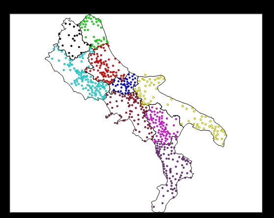
Absent                                  ["kOsa], ["vOk:a]             0
     Present (central-southern origin)       ["kosa], ["vOk:a]             1
     Present (northern origin)               ["kosa], ["vok:a]             -1
4    Word-final vowels                       ‘house’, ‘heart’, ‘eight’,         1
                                             ‘wolf’
     Reduction of all (/@/)                  ["kas@], ["kOr@], ["Ot:@],    0
                                             ["lup@]
     Conservation of -a, reduction of        ["kasa], ["kOr@], ["Ot:@],    1
     others (/a/, /@/)                       ["lup@]
     Conservation of three (/a/,             ["kasa], ["kOre]-["kOri],     2
     /e/-/@/-/i/, /o/-/u/) or four vowels    ["Ot:u], ["lupu]
     (with /i/ distinct from /e/-/@/)
     Conservation of all five vowels         ["kasa], ["kOre], ["Ot:o],    3
     (/a/, /e/, /i/, /o/, /u/)               ["lupu]
5    Alteration of -LL-                      ‘horse’                            1
     Absent (/ll/)                           [ka"val:u]                    0
     Palatal (/j/, /L/, /J/)                 [ka"vaj:u]                    1
     Occlusive (/dd/) and retroflex          [ka"vad:u]                    2
6    Metaphony of -A-                        ‘hands’                            1
     Absent                                  ["man@]                       0
     Present                                 ["min@]                       1
7    Some groups of consonants + L           ‘(it) rains’, ‘white’,             1
                                             ‘flower’
     Standard (/pj/, /bj/, /fj/)             ["pjov@], ["b:jang@],         0
                                             ["fjor@]
     Alteration of /pl/ > /kj/               ["cov@], ["b:jang@],          1
                                             ["fjor@]
     Further alteration of /bl/ > /j/        ["cov@], ["jang@], ["fjor@]   2
     Further alteration of /fj/ > /S/,       ["cov@], ["jang@], ["Sor@]    3
     /x/ etc.
8    Apocope of -no, -ne                     ‘bread’, ‘wine’                    0.5
     Absent                                  ["pane], ["vino]              0
     Only -ne                                ["pa], ["vino]                1
     Both                                    ["pa], ["vi]                  2
9    Outcomes of -LJ-                        ‘son’                              1
     Palatal (/L/)                           ["fiL@]                       0
     Approximant (/j/)                       ["fij@]                       1
     Occlusive (/é/)                         ["fié@]                       2
10   Aspiration of -F-                       ‘coffee’                           1
     Absent                                  [ka"fe]                       0
     Present                                 [ka"he]                       1
11   Rhotacization of -D-                    ‘tooth’                            1
     Absent                                  ["dEnd@]                      0
     Present                                 ["rEnd@]                      1

                                         5
12 Degemination of -RR- and other ‘ground’ 1
geminates
Absent ["tEr:a] 0
Present (of -rr-) ["tEra] 1
Present (of -rr- and others) ["tEra] 2
13 Postnasal sonorization of stops and ‘spring’, ‘when’ 1
progressive assimilation in groups
of /n/ + stops
Both present ["fonde], ["kwan:o] 0
Only assimilation ["fonte], ["kwan:o] 1
Both absent ["fonte], ["kwando] 2
14 “Florentine” Anaphonesis ‘tongue’ 1
Absent ["leNgwa] 0
Present ["liNgwa] 1
15 Some groups of consonants + J ‘arm’, ‘to eat’, ‘to go 1
out’
Standard (/Ù/, /ñ/, /j/) ["vraÙ:@], [ma"ñ:a], ["ji] 0
Alteration of /kj/ > /ţ/ ["vraţ:@], [ma"ñ:a], ["ji] 1
Further alteration of /ngj/ > /nÃ/ ["vraţ:@], [ma"nÃa], ["ji] 2
Further alteration of /j/ > /S/ ["vraţ:@], [ma"nÃa], ["Si] 3
16 Group R + J ‘baker’ 1
Central-southern /r/ [for"naro] 0
Tuscan /j/ [for"najo] 1
17 Group S + J ‘kiss’ 1
Postalveolar (/S/) ["vaS@] 0
Alveolar (/s/) ["vas@] 1
18 Tonic vowel system ‘snow’, ‘month’, ‘cross’ 1
Common Romance ["nev@], ["mes@], ["kroÙ@] 0
“Romanian” ["nev@], ["mes@], ["kruÙ@] 1
“Sardinian” ["niv@], ["mEs@], [’kruÙ@] 2
“Sicilian” ["niv@], ["mis@], ["kruÙ@] 3
Traditionally, most of these features are associated with “isoglosses” that
have been used to define dialect groups or subgroups. For instance, trait no. 4
is the definitory isogloss that separates the Central dialects from Intermediate-
Southern dialects in the classification of Pellegrini.
All varieties in the geographical space considered have been inspected and
attributed a numerical value for each trait. Traits that have just two outcomes
can generate either a digit 0 (in general, absence of that trait) or 1 (presence).
Traits with multiple (P ) outcomes can generate digits ranging from 0 to P −
1 where 0 is generally attributed to the “most standard” outcome, and the
digit increases with the degree of deviation from this standard. The numerical
values of each outcome are equally listed in Table 1. In case of intermediate,
simultaneous, or uncertain outcomes, sometimes fractional values have been
6Figure 1: Localization of the homogeneous areas (circles). Each colour corre-
sponds to one of the administrative regions. Boundaries between regions are
drawn.
used.
Resulting from this transcription, each dialect corresponds to a string of L
digits, {xℓ }L
1 . Varieties that are geographically adjacent and share the same
string are considered as equal and form a “homogeneous area” (HA) for the
purposes of this study. In the whole space, no less than N = 628 homogeneous
areas have been identified in this way: 108 in Latium, 89 in Calabria, 88 in the
Abruzzi, 83 in Campania, 79 in Basilicata, 76 in Apulia, 40 in Molise, 44 in the
Marches, 21 in Umbria. The localization of these areas is shown schematically
in Fig. 1. Their actual extension and the varieties included in each of them are
detailed in the companion web site.
Each homogeneous area represents one point in the data set used for the
classification. The metrics used is the Manhattan distance
X
Dij = wℓ |xiℓ − xjℓ |, (1)
ℓ
where | · | denotes the absolute value and w is a vector of weights. In this study,
wℓ is always 1 except for ℓ = {1, 2, 8} where w = 0.5 has been used, see Table
71. We note that this procedure is roughly equivalent to ‘count the isoglosses’
between two different locations.
Based on this metric, a k-means algorithm has been used to classify the
N L-dimensional points into K groups. This well-known algorithm tries to
attribute each point to one of the clusters by minimising the within-cluster sum
of Manhattan distances, that is,
K X X
X L
min wℓ |xiℓ − mkℓ |, (2)
k=1 xi ∈Ck ℓ=1
where the centroid mk is defined as the mean of points belonging to cluster k
(Ck ),
1 X
mk = xj . (3)
card(Ck )
xj ∈Ck
In practice, the algorithm proceeds iteratively. First, a set of K means is
randomly generated. Then, each point is attributed to the cluster with the
‘nearest’ mean. Further, means are recalculated based on the points attributed
to each cluster. This process is repeated for T iterations. However, the algorithm
is not guaranteed to find the optimum, i.e., the clustering that minimizes the
objective in (2) [Russel & Norvig, 2020]. For this reason, the algorithm is run
for R times, each time with a different (random) initialization of the means.
For each run, the objective is calculated and finally the run with the minimal
objective is chosen as the result. For this study, the algorithm is parametrized
with T = 20 and R = 200K.
To choose the optimal number of clusters K, the silhouette analysis is used.
According to this method, a silhouette metric is defined as a function of the
number of clusters as
bi − ai
σ(K) = (4)
max(ai , bi )
where ⟨·⟩ denotes the average over all points i, and
1 X 1 X
ai = Dij , bi = min Dij (5)
card(CI ) − 1 J̸=I card(CJ )
j∈CI ,j̸=i j∈CJ
are the mean distance between point i and all other points in the same cluster CI
and the smallest mean distance of i to all points in any other cluster, respectively.
The optimal number of clusters is chosen as to maximise the silhouette. The
silhouette coefficient SC = maxK σ(K) summarizes the final result.
It is common opinion that belonging to one particular dialectal group is not a
rigid attribute, but instead, transition bands exist. To retrieve this intuitive be-
haviour in a quantitative way, we have used the following method. We compute
the distance between each HA and the centroids of all clusters,
X
Dik = wℓ |xiℓ − mkℓ |. (6)
ℓ
8The lowest distance corresponds by definition to the cluster k to which the
HA is member. If the difference between the second lowest distance (say, with
cluster h) and the lowest distance is less than a specified fraction of the lowest
distance, then that HA is marked as a transitional area between cluster k and
cluster h,
\
i ∈ CKH if Dih < Diℓ ,∀ℓ ̸= {k, h} Dih < (1 + ξ)Dik . (7)
3 Data
Data for all varieties considered have been collected from multiple and diverse
sources, including material covering the phonetics of specific varieties (see Se-
lected Sources: Specific Varieties), larger areas or entire regions (see Selected
Sources: Larger Areas), comprehensive monographies (see Selected Sources:
Comprehensive Monographies) and linguistic atlases (see Selected Sources: Lin-
guistic Atlases) including acoustic atlases. Other acoustic material available on
the web, both ethnographic and spontaneous, has also provided data for cer-
tain dialectal traits. Good dialectal dictionaries, although often written by
non-professional researchers, have been found for many varieties. Dialectal lit-
erature (mostly, poetry) in specific varieties and collections covering broader
areas have been also perused, particularly for those traits that are unambiguous
when written. Many of these non-scholarly sources are listed in the compan-
ion website. Less canonically, many data have been obtained by inspecting,
searching, and sometimes querying dialect-oriented groups in social networks
such as Facebook. Older scholarly data have been systematically checked in the
(written) conversations found in these groups.
As a result, a database containing thousands of observations has been pre-
pared and is available to the readers upon request to the author. Based on that,
the strings for each variety have been constructed and the homogeneous areas
identified.
Inspection of unclassified results provides already some useful insight. For
instance, it is possible to graphically represent on a map the distances from a
given HA, creating similarity maps as defined in [Goebl et al., 2019]. Moreover,
“isogloss maps” and “beam maps” have been also created. Examples of the
latter for all regions considered are shown in the companion website, where only
‘beams’ corresponding to distances D ≤ 1 are plotted, depicting the emergence
of dialectal continua. However, this analysis yields many small continua and a
large number of isolated areas (whose distance with all conterminous areas is
larger than 1), making a significant classification impossible. For this purpose,
the most useful analysis is that of clustering, which is presented in the next
section.
94 Results
Clustering with several values of K ranging from 2 to 11 have been run and
inspected. For higher values of K the overall results become very sensitive to the
random initialization, unstable, and thus are not shown. Table 2 summarizes
the main divides (traditionally, the “isoglosses”) that characterize each new
partition, as well as the new groups that emerge from it.
The silhouette factor as a function of K is shown in 2. Values are given as
the mean of four series of runs plus/minus the standard deviation. When the
latter is small, it means that the results are stable when different series of runs
are executed. As it can be observed, the factor σ generally decreases with the
number of clusters, with the coincidence intervals of two consecutive K that are
generally not overlapping. However, two values of K emerge as local maxima,
namely, K = 2 and 4. A third cluster number, K = 9 has a mean silhouette
factor that is close to that with K = 8. Moreover, there is an overlap of the
respective confidence intervals, which means that for some series of runs the
silhouette could be higher with K = 9 than with K = 8.
Table 2: Clustering results as a function of the no. of clusters K.
New groups in bold.
K Main new divide (w.r.t. Groups identified σ
K − 1)
2 Salerno-Lucera-Vieste Northern space vs. 0.400 ± 0.000
(SLV) Southern space
3 Gaeta-Sora-Termoli (GST), Northern, Central, 0.361 ± 0.002
Alento-Agri-Taranto- Southern subspaces
Brindisi
4 GST, SLV, Alento-Crati- Northern, 0.365 ± 0.000
Nardò-Brindisi Central-Northern,
Central-Southern,
Southern subspaces
5 Sora-L’Aquila-S. Benedetto Northern subspace, 0.341 ± 0.000
Abruzzese,
Central-Northern,
Central-Southern,
Southern subspaces
6 Foggia-Potenza-Cassano Northern subspace, 0.329 ± 0.003
Abruzzese,
Central-Northern subspace,
Apulian,
Irpino-Lucanian,
Southern subspace
100.4
silhouette coefficient
0.38
0.36
0.34
0.32
0.3
2 4 6 8 10
K
Figure 2: Silhouette coefficient as a function of the number of groups.
7 Pollino-Sila-Lamezia Northern subspace, 0.321 ± 0.002
Abruzzese,
Central-Northern subspace,
Apulian, Irpino-Lucanian,
Cosentino,
Salentino-Calabrian
8 Latina-Ancona Perimedian, Median, 0.315 ± 0.003
Abruzzese,
Central-Northern subspace,
Apulian, Irpino-Lucanian,
Cosentino,
Salentino-Calabrian
9 irregular Perimedian, Median, 0.311 ± 0.001
Abruzzese, Samnite,
Neapolitan-Molisano,
Apulian, Irpino-Lucanian,
Cosentino,
Salentino-Calabrian
10 Irregular As above, but 0.308 ± 0.001
Irpino-Lucanian split in
two groups
11 Irregular As above, but 0.304 ± 0.002
Marsican-Southern Latian
split from Abruzzese
11Table 3: List of Province codes. Regional capital cities in bold.
THE MARCHES (Marche) CAMPANIA
Ancona AN Avellino AV
Ascoli Piceno AP Benevento BN
Fermo FM Caserta CE
Macerata MC Napoli NA
UMBRIA Salerno SA
Perugia PG APULIA (Puglia)
Terni TN Bari BA
LATIUM (Lazio) Barletta-Andria-Trani BT
Frosinone FR Brindisi BR
Latina LT Foggia FG
Rieti RI Lecce LE
Roma RM Taranto TA
Viterbo VT BASILICATA
ABRUZZI (Abruzzo) Matera MT
L’Aquila AQ Potenza PZ
Chieti CH CALABRIA
Pescara PE Cosenza CS
Teramo TE Catanzaro CZ
MOLISE Crotone KR
Campobasso CB Reggio di Calabria RC
Isernia IS Vibo Valentia VV
The first optimal classification with K = 2 divides the overall space con-
sidered into a Northern and a Southern space, separated by a line that resem-
bles the traditional Salerno-Lucera (actually, Salerno-Lucera (FG)-Vieste (FG),
SLV) isogloss bundle. For instance, around this line lays the northern limit of
KJ > /ţ:/ (see trait 15 in Table 1).
In the partition with K = 4 each of these subspaces split in two. Thus,
a Northern subspace is separated from a Central-Northern subspace by a line
running from around Gaeta (LT) on the Tyrrhenian coast to around Termoli
(CB) on the Adriatic coast, with an elbow around Sora (FR). The Central-
Northern subspace is separated from a Central-Southern subspace by a SLV line,
although not exactly coincident with the previous one. Finally, the Central-
Southern subspace is separated from a Southern subspace by two lines, one
running from around the mouth of the Alento river (SA) on the Tyrrhenian
coast to the mouth of the Crati river (CS) on the Ionian coast, the other running
from around Nardò (LE) on the Ionian coast to around Brindisi on the Adriatic
coast.
A further relevant partition is obtained with K = 9, not only because a
substantial plateau of σ is observed, but also because the results are more stable
than with K = 7 or K = 8 (lower std). Incidentally, this value of K matches
the number of administrative regions (Regioni) in the space considered. This
partition could be thus a promising basis for the definition of more accurate
12“regional languages” in this half of Italy. The groups identified by clustering
with K = 9 are listed in Table 2 and detailed here from North to South as:
1. “Perimedian” group, including provincial capitals AN, PG, VT, RM, LT,
and areas in Northern Marches, in Central-Western Umbria, in Western
Latium, besides a hamlet (frazione) in Basilicata (a Marchigiano colony).
2. “Median” group, including provincial capitals MC, FM, TN, RI, FR, AQ,
and areas in Central Marche, South-Eastern Umbria, Central Latium,
Western Abruzzi.
3. “Abruzzese” group, including provincial capitals AP, TE, PE, CH, and
areas in Southern Marche, Eastern Abruzzi, Southern Latium, besides
two smaller areas in Molise.
4. “Samnite” group, including provincial capitals IS, CB, BN, and areas in
South-Eastern Latium, Western Molise, Northern Campania, besides some
smaller areas in Campania, Northern Apulia, and Basilicata around and
including the provincial capital PZ (Gallo-Italic colonies).
5. “Neapolitan-Molisano” group, including provincial capitals NA, CE, SA,
and areas in Central Campania, Eastern Molise, besides some smaller
areas in North-Western Apulia.
6. “Apulian” group, including provincial capitals FG, BAT, BA, TA, MT,
BR, and areas in Northern-Central Apulia, South-Eastern Basilicata, North-
Eastern Calabria, besides some smaller areas in Central Campania.
7. “Irpino-Lucanian” group, including provincial capital AV and areas in
Southern-Eastern Campania, Western Basilicata, and North-Eastern Apu-
lia.
8. “Cosentino” group, including provincial capital CS and areas in Southern
Campania (likely having a Greek substratum), Northern Calabria, besides
some smaller areas in Basilicata (most of them being or having been Gallo-
Italic colonies).
9. “Salentino-Calabrian” group, including provincial capitals LE, KR, VV,
CZ, RC, and areas in Southern Apulia and Central-Southern Calabria,
besides some smaller areas in Northern Calabria.
Figure 3 shows the attribution of each HA to one of the nine clusters, iden-
tified by a colour. It must be noted that the k-means algorithm has no knowl-
edge about the spatial correlation between the HA, each of them representing
a “point” in an 18-dimensioned space, with these points that can be geograph-
ically ordered in any arbitrary way. Though, the spatial consistency of the
results is striking, and the groups obtained clearly recall traditional regions and
dialectal groups. The actual boundaries between the nine groups can be traced
on a map as depicted in Fig. 4.
13Figure 3: HA clustered in K = 9 groups: schematic representation.
Each colour corresponds to one group: blue (Perimedian), purple (Median),
pink (Abruzzese), red (Samnite), orange (Neapolitan-Molisano), green (Apu-
lian), yellow (Irpino-Lucanian), grey blue (Cosentino), light blue (Salentino-
Calabrian).
14Figure 4: HA clustered in K=9 groups: a linguistic map with actual group
boundaries. Colours of groups correspond to those of Fig. 3
15Boundary between groups 1–2 recalls a well-known isogloss, the Northern
limit of simultaneous /nt/ > /nd/ and /nd/ > /nn/ (see trait 13 in Table 1)
that traditionally separates the Central Italian dialects into a “Perimedian”
and a “Median” section (whence the naming of groups 1 and 2 used here).
Boundary 2–3 runs similarly to another definitory isogloss, the Northern limit
of [@] (see trait 4 in Table 1), which serves to separate Central from Southern
(“Neapolitan language”) dialects in traditional classifications. Boundary 3–4,
or the GST bundle introduced above, is similar to the Northern limit of PL
> /kj/ (see trait 7 in Table 1) or isogloss 21 in Pellegrini’s map. Boundary
between 4, 5 on one side and 6, 7 on the other, is the SLV bundle discussed
above. Boundary between 6, 7 on one side and 8, 9 on the other, recalls the
Northern limit of non-standard tonic vowel systems (trait 18 in Table 1), which
is different from isogloss 25 (Southern limit of [@]) that is traditionally used to
separate the Intermediate Southern dialects from the Extreme Southern dialects
(“Sicilian” language). Finally, the North-South boundary between groups 7, 8
on one side and 6, 9 on the other, matches almost perfectly a less used isogloss,
i.e., the Western limit of LJ > /é/ (see trait 9 in Table 1), whereas in traditional
classifications the corresponding boundaries are purely administrative.
Figures 5 (schematic view) and 6 (pictorial) show the transitional areas
identified with the method (7) of second-best clusters (with ξ = 0.5). These
results suggest the existence of such areas at the geographical boundary between
groups 1 and 2 (in Marche, Umbria, and Latium), 2 and 3 (in Marche, Abruzzi,
and Latium), 2 and 4, 3 and 4 (in Latium), 3 and 5 (in Abruzzi and Molise), 4
and 5 (in Molise, Campania and Apulia), 4 and 7 (in Campania), 5 and 6 (in
Apulia), 6 and 7 (in Apulia and Basilicata), 7 and 8 (in Basilicata), 6 and 8,
6 and 9 (in Apulia and Calabria), 8 and 9 (in Calabria). Again, these results
are consistent with geography in the sense that transitional areas are generally
identified between clusters that actually share a geographical border.
5 Conclusions
In this paper, we have presented a dialectometry-based study aimed at classi-
fying the Romance varieties of Central-Southern Italy. We have analysed the
thousands of varieties under study and operated a massive pre-treatment of data
available from many sources, resulting in a substantial reduction of the problem
dimension. We have characterized these varieties with respect to 18 phonetic
traits, including the isoglosses that have been traditionally used by linguists to
define dialectal groups. On this basis we have identified 628 homogeneous areas
as the groups conterminous varieties that share the same traits. As a result, we
have got an operating data set of 628 points in an 18-dimensional space, where
we could define linguistic distances. We have then formulated the problem as a
clustering problem, that is, find the K clusters of those points that minimise the
within-cluster linguistic distance. We have used a k-means algorithm to cluster
and an ad-hoc rule to define second-best clusters and transitional areas. We
have used silhouette analysis to select the most appropriate number of clusters.
16Figure 5: HA clustered in K=9 groups with second-best clusters: schematic
representation. Core clusters are identified by the left-half colour of the circles;
second-best clusters in transitional area are identified by right-half colours.
17Figure 6: HA clustered in K=9 groups with second-best clusters: a linguistic
map with actual group boundaries and transitional areas (hatched).
18The results are geographically consistent, although the algorithms used have no
information about the actual geographical distance between areas or the bound-
aries shared by them. The methods used suggest that clustering with 9 groups
is the most appropriate choice.
The dialectal groups identified (labelled as Perimedian, Median, Abruzzese,
Samnite, Neapolitan-Molisano, Apulian, Irpino-Lucanian, Cosentino, and Salentino-
Calabrese) resemble but do not coincide with the regional varieties traditionally
invoked. Both hard and fuzzy boundaries between them are based only on lin-
guistic considerations, and not administrative or historical boundaries. Often
these boundaries coincide at least partially with known isoglosses, suggesting
a high linguistic consistency of the results. We conclude that a classification
based on these grounds is less arbitrary than traditional ones based on selected
isoglosses as it considers multiple dialectal traits. It is also less subjective since
the partitioning is made by an algorithm that tries to minimise a clearly defined
objective function. Another strength of the method is that it can be readily
adapted as long as new data is available, varieties evolve, or corrections are
made to the data set.
References
[Burridge et al., 2019] Burridge, James, B. Vaux, M. Gnacik, & Y. Grudeva.
2019. Statistical physics of language maps in the USA. Phys. Rev. E.
99:032305.
[Cheshire et al., 2011] Cheshire, J. A., P. Mateos, & P.A. Longley. 2011. Delin-
eating Europe’s cultural regions: population structure and surname clus-
tering. Hum. Biol. 83. 573–598.
[Eberhard et al. 2022] Eberhard, David M., G.F. Simons, & C.D. Fennig (eds.).
2022. Ethnologue: Languages of the World. Twenty-fifth edition. Dallas,
Texas: SIL International. Online version: http://www.ethnologue.com.
[Goebl, 1982] Goebl, Hans. 1982. Dialektometrie, vol. 157. Vienna: Verlag der
Osterreichischen Akademië der Wissenschaften.
[Goebl, 2008] Goebl, Hans. 2008. Le Laboratoire de dialectométrie de
l’Université de Salzbourg. Un bref rapport de recherche. Zeitschrift für
französische Sprache und Literatur 118(1). 35–55.
[Goebl, 2010] Goebl, Hans. 2010. Dialectometry and quantitative mapping. In
A. Lameli, R. Kehrein, & S. Rabanus (eds.), Language and Space. An Inter-
national Handbook of Linguistic Variation, Volume 2: Language Mapping,
433–457. Berlin & New York: de Gruyter.
[Goebl, 2018] Goebl, Hans. 2018. Dialectometry. In Boberg, C, J. Nerbonne &
D. Watt (eds.), The handbook of dialectology, 123-142. Oxford: Wiley.
19[Goebl et al., 2019] Goebl, Hans, Edgar Haimerl, Pavel Smečka, Bernhard
Castellazzi, & Yves Scherrer. 2019. Dialectometry AIS. Retrieved from
http://dialektkarten.ch/dmviewer/ais/index.en.html.
[Hammarström et al., 2022] Hammarström, Harald, R. Forkel, M. Haspelmath
& S. Bank, 2022. Glottolog 4.6. Leipzig: Max Planck Institute for Evolu-
tionary Anthropology. Online version http://glottolog.org
[Heeringa, 2004] Heeringa, W.J. 2004. Measuring Dialect Pronunciation Differ-
ences using Levenshtein Distance. Ph.D. dissertation. Groningen: Univer-
sity of Groningen.
[Hyvönen et al., 2007] Hyvönen, Saara, Antti Leino, & Marko Salmenkivi.
2007. Multivariate analysis of Finnish dialect data—an overview of lexi-
cal variation. Literary and Linguistic Computing 22(3). 271–290.
[Jaberg & Jud, 1987] Jaberg, Karl & Jacob Jud. 1987. Atlante linguistico ed
etnografico dell’Italia e della Svizzera meridionale (AIS). Milano: Unicopli.
Retrieved from NavigAIS-web, https://navigais-web.pd.istc.cnr.it/
[Levenshtein, 1966] Levenshtein, Vladimir I. 1966. Binary codes capable of cor-
recting deletions, insertions, and reversals. Soviet Physics Doklady 10(8).
707–10.
[Montemagni & Wieling, 2016] Montemagni, Simonetta & Martijn Wieling.
2016. Tracking linguistic features underlying lexical variation patterns: A
case study on Tuscan dialects. In Côté, M.-H., R. Knooihuizen & J. Ner-
bonne (eds.). The future of dialects, 117-135. Berlin: Language Science
Press.
[Moseley, 2010] Moseley, Christopher (ed.). 2010. Atlas of the World’s Lan-
guages in Danger (3rd edition). UNESCO Publishing. Online version
https://unesdoc.unesco.org/ark:/48223/pf0000187026
[Nerbonne et al., 2021] Nerbonne, John, W.J. Heeringa, Jelena Prokić & Mar-
tijn Wieling. 2021. Dialectology for computational linguists. In Zampieri,
M. & P. Nakov (eds.), Similar languages, varieties, and dialects: A compu-
tational perspective, Studies in Natural language processing, 96-118.
[Pellegrini, 1977] Pellegrini, Giovan Battista. 1977. Carta dei dialetti d’Italia.
Pisa: Pacini.
[Pickl, 2014] Pickl, Simon, Aaron Spettl, Simon Pröll, Stephen Elspass, Werner
König, & Volker Schmidt. 2014. Linguistic Distances in Dialectometric In-
tensity Estimation. Journal of Linguistic Geography 2(1). 25-40.
[Pröll et al., 2014] Pröll, Simon, Pickl, Simon, & Spettl, Aaron. 2014. Latente
Strukturen in geolinguistischen Korpora. In Michael Elmentaler, Markus
Hundt, & Jürgen Erich Schmidt (eds.), Deutsche Dialekte. Konzepte, Prob-
leme, Handlungsfelder. Akten des, 4., vol. 4, 247–58. Stuttgard: Steiner.
20[Romano et al., 2022] Romano, Noemi, P. Ranacher, S. Bachmann & Stéphane
Joost. 2022. Linguistic traits as heritable units? Spatial Bayesian cluster-
ing reveals Swiss German dialect regions. Journal of Linguistic Geography
10(1). 11-22.
[Russel & Norvig, 2020] Russel, Stuart & Peter Norvig. 2020. Artificial Intelli-
gence: A Modern Approach. Englewood Cliffs, NJ: Prentice Hall.
[Séguy, 1973] S’eguy, Jean. 1973. La dialectométrie dans l’Atlas linguistique de
la Gascogne. France: Société de linguistique romane.
[Syrjanen et al., 2016] Syrjänen, Kaj, Terhi Honkola, Jyri Lehtinen, Antti Lein
& Outi Vesakoski. 2016. Applying Population genetic approaches within
languages. Language dynamics and change 6. 235-283.
[Valls et al., 2012] Valls, Esteve, Nerbonne, John, Prokić, Jelena, Wieling, Mar-
tijn, Clue, Esteve, & Rosa Lloret, Maria. 2012. Applying the Levenshtein
Distance to Catalan dialects: A brief comparison of two dialectometric
approaches. Verba: anuario galego de filoloxia 39. 35–61.
[Wieling & Nerbonne, 2011] Wieling, Martijn & John Nerbonne. 2011. Bipar-
tite spectral graph partitioning for clustering dialect varieties and detecting
their linguistic features. Computer Speech and Language 25. 700-715.
[Wieling et al., 2013] Wieling, Martijn, R.G. Shackleton & John Nerbonne.
2013. Analyzing phonetic variation in the traditional English dialects: Si-
multaneously clustering dialects and phonetic features. Literary and Lin-
guistic Computing 28(1). 31-41.
[Wieling et al., 2014] Wieling, Martjin, J. Bloem, K. Mignella, M. Timmermeis-
ter, & John Nerbonne. 2014. Validating and using the PMI-based Leven-
shtein distance as a measure of foreign accent strength. Poster presented
at Methods in Dialectology XV, Groningen (The Netherlands).
Selected Sources
Specific Varieties
1. Abete, Giovanni. 2006. Sulla questione della sillaba superpesante: I dit-
tonghi discendenti in sillaba chiusa nel dialetto di Pozzuoli. In Savy, R. &
C. Crocco (eds.), Atti del II Convegno Nazionale dell’Associazione Italiana
di Scienze della Voce (AISV), 379-398. Torriana: EDK.
2. Abete, Giovanni. 2020. Nuove acquisizioni sul vocalismo marginale: il
dialetto di Calitri (AV). L’Italia dialettale 81. 311-339.
3. Avolio, Francesco & Antonio Romano. 2010. Ai margini dell’area Laus-
berg: le varietà di Aliano e Alianello nei risultati di un’indagine dialet-
tologica e fonetica. In Iliescu, M., H.-S. Runggaldier & P. Danler (eds.),
21Actes du XXVe Congrès International de Linguistique et de Philologie
Romane, vol. 4, 25-36. Berlin: De Gruyter.
4. Ceppaglia, Marco & Antonio Romano. 2018. Il dialetto di Martina Franca
da G. Grassi a G.G. Marangi: analisi fonetica descrittiva del vocalismo.
L’idomeneo 25. 241-250.
5. Colonna, Valentina & Antonio Romano. 2018. La variazione diatopica
nel micro-spazio dialettale leccese: il dialetto salentino delle frazioni di
Vernole. In Caramuscio, G. & A. Romano (eds.), Una d’arme, di lingua,
d’altare, di memorie, di sangue, di cor: omaggio a Luciano Graziuso.
Lecce: Grifo.
6. Costagliola, Angelica. 2007. Il vocalismo tonico di Lecce: analisi Acustica
di un campione di parlanti differenziati per sesso ed età. Atti del I Con-
gressso Nazionale dell’Associazione Italiana di Scienze della Voce (AISV),
567-596.
7. D’Alessandro, Roberta & Marc van Oostendorp. 2014. La metafonia
fra fonologia e lessico: Il caso dell’ariellese. In Pescarini, Diego & Diana
Passino (eds.), Studi sui dialetti dell’Abruzzo. Quaderni di lavoro ASIT
17, 1-18.
8. D’Andrea, Federica, Carmela Lavecchia, Francesca V. Russo, Carminella
Scarfiello, Anna M. Tesoro & Francesco Villone. 2016. I dialetti: patri-
moni culturali locali nella lingua (rivista di proietti dottorali in Corso).
Ianua. Revista Philologica Romanica 17. 133-168.
9. De Iacovo, Valentina. 2018. Il dialetto di Leporano (TA): un confronto tra
un’inchiesta dialettale recente e l’inchiesta della Carta dei Dialetti Italiani.
L’idomeneo 25. 215-222.
10. Ferrari-Bridgers, Franca. 2010. The Ripano dialect: Toward the end of
a mysterious linguistic island in the heart of Italy. In Millar, Robert Mc-
Coll (ed.). Marginal Dialects: Scotland, Ireland and Beyond. Aberdeen:
Forum for Research on the Languages of Scotland and Ireland. 106-130.
11. Gaglia, Sascha. 2007. Metaphonie im kampanischen Dialekt von Piedi-
monte Matese. Ph.D. dissertation. Konstanz: Universität Konstanz.
12. Hončová, Marketa. 2011. La scelta del verbo ausiliare nei dialetti di
Corropoli e Nereto. Ph.D. dissertation. Praha: Univerzita Karlova.
13. Iannacito, Roberta. 2002. L’assimilazione progressive nel dialetto molisano
di Villa San Michele (IS). Italica 79(4). 509-524.
14. Iannacito-Provenzano, Roberta. 2005. Cenni sulla frase ipotetica in due
dialetti dell’Alto Molise. Forum Italicum: A Journal of Italian Studies
39(2). 498-519.
2215. Idone, Alice & Giuseppina Silvestri. 2018. Verbicarese. Zurich: Univer-
sität Zürich. Retrieved from http://www.dai.uzh.ch/new/#/public/
overviews
16. Loporcaro, Michele & Dafne Pedrazzoli. 2016. Classi flessive del nome e
genere grammaticale nel dialetto di Agnone (Isernia). Revue de Linguis-
tique Romane (RLiR) 80(317). 73-100.
17. Lupini, Carmelo. 2004. Frangimenti e turbamenti di “a” tonica nella
Calabria centro-settentrionale: il dialetto di Acri. Atti del convegno su
Padula, la Calabria, l’Italia: nuovi orizzonti della ricerca paduliana (Roc-
cella Jonica, Italy, March).
18. Maggiore, Marco & Angelo Variano. 2015. Differenziazione vocalica per
posizione e differenziazione fonetica su base sessuale nella varietà di Zap-
poneta (FG). L’Italia dialettale 76. 83-104.
19. Mancarella, Giovan Battista. 2018. L’attività Contadina narrate nel di-
aletto di Sava. L’idomeneo 25. 133-146.
20. Paciaroni, Tania & Michele Loporcaro. 2007. Funzioni morfologiche
dell’opposizione fra -u e -o nei dialetti del maceratese. In Iliescu, M.,
H. Siller-Runggaldier & P. Danler (eds.), Actes du XXVe Congrès Inter-
national de Linguistique et de Philologie Romanes, 497-506. Innsbruck
(Austria).
21. Paciaroni, Tania. 2009. Coarticolazione e mutamento: una ricerca sul vo-
calismo atono finale nell’entroterra maceratese. In Schmid, S., M. Schwarzen-
bach & D. Studer (eds.), La dimensione temporale del parlato: Atti del 5°
convegno nazionale AISV, 177-194. Zürich: Phonetisches Laboratorium.
22. Paciaroni, Tania. 2012. Dialecte et italien standard à Macerata: du côté
du locuteur. In Léonard, J.L. & K.J. Avilés Gonzáles (eds.), Documen-
tation et revitalisation des “langues en danger”: épistémiologie et praxis.
Paris: Houdiard. 327-369.
23. Passino, Diana & Diego Pescarini. 2018. Il Sistema vocalico del dialetto
alto-meridionale di San Valentino in Abruzzo Citeriore con particolare
riferimento agli esiti di Ū. In Antonelli, Roberto, Martin Glessgen & Paul
Visdott (eds.), Proc. of the XXVIII Congresso internazionale di linguistica
e filologia romanza, 484-497. Roma.
24. Patrascu, Francesca-Alessandra. 2019. Dialetto e italiano regionale ad
Assisi. Mag. Phil. Dissertation. Vienna: Universität Wien.
25. Radtke, Edgar. 1997. Tortorella: eine bislang unbekannte galloitalienische
Sprachkolonie im Cilento. Zeitschrift für romanisce Philologie 113(1). 82-
108.
2326. Romano, Antonio. 2010. Norma e variazione nel dialetto salentino di
Parabita. In Spedicato, M. (ed.), Scritti in memoria di Oronzo Parlangeli
a 40 anni dalla scomparsa (1969-2009), 237-268. Galatina: EdiPan.
27. Romano, Antonio. 2013. Il vocalismo del dialetto salentino di Galatone:
differenze d’apertura metafonetiche, trace isolate di romanzo commune e
interferenze diasistematiche. In Romano, A. & M. Spedicato (eds.), Sub
voce Sallentinitas: Studi in onore di G.B. Mancarella, 247-276. Lecce:
Grifo.
28. Russo, Michela. 2010. Le origini della dittongazione spontanea nei dialetti
italiani meridionali dell’ovest (Ischia e Pozzuoli): Isocronia diacronica an-
tischürriana e quantificazioni isocroniche attuali. Zeitschrift für Romanis-
che Philologie 126(2). 304-349.
29. Schirru, Giancarlo. 2016. Propagginazione e flessione nominale in al-
cuni dialetti italiani centro-meridionali. Atti del Sodalizio Glottologico
Milanese 8-9. 121-130.
30. Sornicola, Rosanna. 1999. Alcune recenti ricerche sul parlato: le di-
namiche vocaliche di € nell’area flegrea e le loro implicazioni per una
teoria della variazione. In Dardano, M., A. Pelo & A. Stefinlongo (eds.),
Atti del colloquio internazionale di studi Scritto e parlato: metodi, testi e
contesti, 239-264. Roma.
31. Sornicola, Rosanna. 1999. La variazione dialettale nell’area costiera napo-
letana: il Progetto di un Archivio di testi dialettali parlati. In Marcato,
G. (ed.), Dialetti oggi, Atti del convegno Tra lingua, cultura, società: di-
alettologia sociologica (Sappada-Plodn 1-4 luglio 1999), 103-122. Padua:
Unipress.
32. Villone, Francesco. 2018. Tra micro e macro aree: elementi linguistici
ed extra-linguistici nel case study Avigliano alla luce dei dati dell’Atlante
Linguistico della Basilicata (A.L.Ba). In Sampino, G. e F. Scaglione (eds.),
Saperi umanistici nella contemporaneità, Atti del convegno internazionale
dei dottorandi (Palermo, Italy, 17-18 Sept. 2015), 161-177. Palermo:
Palumbo.
33. Vitolo, Giuseppe. 2005. L’ausiliare nei dialetti di Salerno, Cetara, Cas-
tiglione dei Genovesi e Salitto. Quaderni del Dipartimento di Linguistica
15, 238-254. Firenze: Università di Firenze.
34. Vitolo, Giuseppe. 2017. Fenomeni fonetici e morfo-sintattici del dialetto
campano di Pagani. Quaderni di Linguistica e Studi Orientali 3. 219-241.
Larger Areas
1. Abete, Giovanni. 2011. I processi di dittongazione nei dialetti dell’Italia
meridionale: un approccio sperimentale. Roma: Aracne.
242. Abete, Giovanni. 2017. Parole e cose della pastorizia in Alta Irpinia.
Napoli: Giannini.
3. Avolio, Francesco. 1995. Note sulla variabilità linguistica nell’Appennino
abruzzese. Nouvelles du Centre d’Etudes Francoprovençales René Willien,
Mélanges en souvenir de Marco Perron 31. 91-105.
4. Avolio, Francesco. 2010. I dialetti dell’area cassinese e dell’odierno basso
Lazio: alcune considerazioni. Quaderni Coldragonesi 1. 27-36.
5. Balducci, Sanzio. 1987. I dialetti. In Anselmi, S. (ed.), La provincial di
Ancona: storia di un territorio, 273-284. Bari: Laterza.
6. Cangemi, Francesco, Rachele Delucchi, Michele Loporcaro & Stephan
Schmid. 2010. Vocalismo finale atono “toscano” nei dialetti del Vallo
di Diano (Salerno). In Cutugno, F., P. Maturi, R. Savy, G. Abete, &
I. Alfano (eds.), Parlare con le persone, parlare alle machine, 477-490.
Torriana: EDK.
7. Capotosto, Silvia. 2011. La palatalizzazione di -LL- e -L- nel quadro
linguistico mediano. Contributi di filologia dell’Italia mediana 25. 275-
300.
8. Carosella, Maria. 1999. La metafonesi nei dialetti garganici nord-occidentali.
Quaderni del Dipartimento di Linguistica, Università di Firenze 9. 97-138.
9. Castagna, Raffaele (ed.). 2006. I dialetti d’Ischia nella tesi di laurea di
Ilse Freund elaborate dopo un soggiorno a Serrara Fontana (1929). La
rassegna d’Ischia 1.
10. Cimarra, Luigi & Francesco Petroselli. 2001. Proverbi e detti proverbiali
della Tuscia viterbese. Viterbo: Gruppo interdisciplinare per lo studio
della cultura tradizionale dell’Alto Lazio.
11. Corsi, Anna, Valentina Cardinale & Vincenzo Luciani. 2014. Dialetto e
poesia nei 33 comuni della provincia di Latina. Roma: Cofine.
12. Di Carlo, Miriam. 2015. Né toscani né romani: per una caratterizzazione
dei dialetti dell’area viterbese. In Marcato, G. (ed.), Dialetto parlato,
scritto, trasmesso, 345-352. Padua: CLEUP.
13. Egidi, Francesco. 1965. Dizionario dei dialetti piceni fra Tronto e Aso.
Montefiore dell’Aso.
14. Garrapa, Luigia. Vocali maschili e femminili fra Salentocentrale e Salento
meridionale: problemi sincronici per un’analisi diacronica. Atti del I Con-
gressso Nazionale dell’Associazione Italiana di Scienze della Voce (Padova,
Italy, 2-4 Dec. 2004), 651-669.
2515. Germani, Alfonso. 2014. Il tipo dialettale del Lazio meridionale: alcuni
fenomeni linguistici caratteristici. In Lucrările celui de-al XV-lea Sim-
pozion Internat, ional de Dialectologie, 135-165. Cluj-Napoca: Argonaut,
Scriptor.
16. Granatiero, Francesco. 2012. Vocabolario dei dialetti garganici. Foggia:
Grenzi.
17. Grimaldi, Mirko. 2001. Ancora sulla questione del vocalismo siciliano alla
luce di processi metafonetici scoperti nel Salento meridionale. In Quaderni
del Dipartimento di Linguistica 11, 69-105. Firenze: Università di Firenze.
18. Loporcaro, Michele. 2009. Opposizioni di caso nel pronome personale: i
dialetti del mezzogiorno in prospettiva romanza. In De Angelis, A. (ed.),
I dialetti italiani meridionali tra arcaismo e interferenza, Atti del Con-
vegno internazionale di Dialettologia (Messina, 4-6 June 2008), 207-235.
Palermo.
19. Maiden, Martin. 1987. New perspectives on the genesis of Italian metaphony.
Transactions of the Philological Society 85(1). 38-73.
20. Mancarella, Giovan Battista. 2015. Dialetti salentini. L’idomeneo 19.
147-156.
21. Melillo, Giacomo. 1926. I dialetti del Gargano. Pisa: Simoncini.
22. Memoli, Giovanna. Il patrimonio linguistico del Vallo di Diano. In Aro-
mando, G. (ed.), Per angusta ad augusta 1(2). 110-132.
23. Paggini, Valentina & Silvia Calamai. 2016. L’anafonesi in Toscana: il
contributo degli archivi sonori del passato. Atti del Convegno Associazione
Italiana Scienze della Voce, 155-168. Milano: Officinaventuno.
24. Paternostro, Luigi. 2019. Gli alti Bruzi e Il loro linguaggio. Firenze:
Phasar.
25. Retaro, Valentina & Giovanni Abete. 2016. Sull’importanza delle aree
intermedie: I dialetti del Vallo di Lauro. In Antonelli, R., M. Glessgen &
P. Videsott (eds.), Atti del XXVIII Congresso internazionale di linguistica
e filologia romanza vol. 2, 957-968. Roma.
26. Romano, Antonio. 2015. Una selezione di carte linguistiche del Salento.
L’idomeneo 19. 43-56.
27. Romito, Luciano, Tiziana Turano, Michele Loporcaro & Antonio Mendi-
cino. 1996. Micro e macrofenomeni di centralizzazione nella variazione
diafisica: rilevanza dei dati fonetico-acustici per il quadro dialettologico
calabrese. Fonetica e fonologia degli stili dell’italiano parlato. 14-15.
2628. Romito, Luciano, Vincenzo Galatà, Rosita Lio, Francesca Stillo. 2006. La
metafonia nei dialetti dell’area Lausberg: un’introspezione sulla natura
della sillaba. In Savy, R. & C. Crocco (eds.), Analisi prosodica: teorie,
modelli e sistemi di annotazione. Torriana: EDK.
29. Romito, Luciano & Daniela Gagliardi. 2007. La metafonia in alcuni centri
del Nord Calabria: verso una mappa regionale. In Romito, L., V. Galatà &
R. Lio (eds.), Atti del IV Convegno Nazionale dell’Associazione Italiana
di Scienze della Voce (Arcavacata di Rende, Italy, 30-5 Dec.), 423-436.
Torriana: EDK.
30. Russo, Michela. 2002. Metafonesi opaca e differenziazione vocalica nei
dialetti della Campania. Zeitschrift für romanische Philologie 118(2). 195-
223.
31. Savoia, Leonardo M. & Benedetta Baldi. 2016. Propagation and preserva-
tion of rounded back vowels in Lucanian and Apulian varieties. Quaderni
di Linguistica e Studi Orientali / Working Papers in Linguistics and Ori-
ental Studies 2. 11-58.
32. Trumper, John B. La valle del Savuto e la catena paolana: alcune osser-
vazioni storico-linguistiche, anche sulla ‘presenza longobarda’. Retrieved
from https://lingcal.wordpress.com/letture-varie/
33. Vecchia, Cesarina. 2017. La variazione fonetica degli esiti di -LL- in
Irpinia: Processi di rotacizzazione e di retroflessione nelle varietà dell’alta
valle del Calore. Ph.D. dissertation. Napoli: Università Federico II.
34. Vitolo, Giuseppe. 2012. Parlate campane: la selezione dell’ausiliare e il
sistema clitico. Roma: Aracne.
Comprehensive Monographies
1. Avolio, Francesco. 1995. Bommespr@: profile linguistico dell’Italia centro-
meridionale. San Severo: Gerni.
2. Giammarco, Ernesto. 1968-1979. Dizionario abruzzese e molisano. Roma:
Ateneo.
3. Loporcaro, Michele. 2013. Profilo inguistico dei dialetti italiani. Bari:
Laterza.
4. Loporcaro, Michele. 2021. La Puglia e il Salento. Bologna: Il Mulino.
5. Loporcaro, Michele. 2016. Metaphony and diphthongization in Southern
Italy: Reconstructive implications for sound change in early Romance. In
Torres-Tamarit, F., K. Linke & M. van Oostendorp (eds.). Approaches to
metaphony in the languages of Italy, 55-87. Berlin: De Gruyter.
276. Moretti, Giovanni. 1975. Profilo dei dialetti italiani: Umbria. Pisa:
Pacini.
7. Piemontese, Pasquale (ed.). 1982. La parabola del figliuol prodigo nei
dialetti italiani: I dialetti del Molise. Bari: Università di Bari.
8. Rohlfs, Gerhard. 1966. Grammatica storica della lingua italiana e dei suoi
dialetti, vol. 1 Fonetica. Torino: Einaudi.
9. Vignuzzi, Ugo. 1994. Il volgare nell’Italia mediana. In Serianni, Luca
& Pietro Trifone (eds.), Storia della lingua italiana 3, 329-372. Torino:
Einaudi.
Linguistic Atlases
1. Vivaio acustico delle Lingue e dei Dialetti d’Italia (VIVALDI). 1998-2018.
Retrieved from https://www2.hu-berlin.de/vivaldi/index.php
2. Archivio di parlato – La tramontana e il sole. 2017. Torino: Laboratorio
fonetica sperimentale Arturo Genre (LFSAG). Retrieved from https://
www.lfsag.unito.it/ark/table_ita.html
3. Microcontact. Utrecht: Utrecht University. Retrieved from https://
microcontact.hum.uu.nl
28You can also read