Diel quenching of Southern Ocean phytoplankton fluorescence is related to iron limitation
←
→
Page content transcription
If your browser does not render page correctly, please read the page content below
Biogeosciences, 17, 793–812, 2020
https://doi.org/10.5194/bg-17-793-2020
© Author(s) 2020. This work is distributed under
the Creative Commons Attribution 4.0 License.

Diel quenching of Southern Ocean phytoplankton fluorescence is
related to iron limitation
Christina Schallenberg1 , Robert F. Strzepek1 , Nina Schuback2 , Lesley A. Clementson3 , Philip W. Boyd1,4 , and
Thomas W. Trull1,3
1 Antarctic  Climate and Ecosystems Cooperative Research Centre, University of Tasmania, Hobart, Tasmania, Australia
2 Swiss  Polar Institute, École Polytechnique Fédérale de Lausanne, Lausanne, Switzerland
3 Commonwealth Scientific and Industrial Research Organisation Oceans and Atmosphere Unit, Hobart, Tasmania, Australia
4 Institute for Marine and Antarctic Studies, University of Tasmania, Hobart, Tasmania, Australia

Correspondence: Christina Schallenberg (christina.schallenberg@utas.edu.au)

Received: 26 August 2019 – Discussion started: 4 September 2019
Revised: 10 December 2019 – Accepted: 3 January 2020 – Published: 17 February 2020

Abstract. Evaluation of photosynthetic competency in time          decreasing with increased Fe availability, confirming previ-
and space is critical for better estimates and models of           ous work. The fortuitous presence of a remnant warm-core
oceanic primary productivity. This is especially true for areas    eddy in the vicinity of the study area allowed comparison of
where the lack of iron (Fe) limits phytoplankton productivity,     fluorescence behaviour between two distinct water masses,
such as the Southern Ocean. Assessment of photosynthetic           with the colder water showing significantly lower Fv /Fm
competency on large scales remains challenging, but phyto-         than the warmer eddy waters, suggesting a difference in Fe
plankton chlorophyll a fluorescence (ChlF) is a signal that        limitation status between the two water masses. Again, NPQ
holds promise in this respect as it is affected by, and conse-     capacity measured with the FRRf mirrored the behaviour
quently provides information about, the photosynthetic effi-       observed in Fv /Fm , decreasing as Fv /Fm increased in the
ciency of the organism. A second process affecting the ChlF        warmer water mass. We also analysed the diel quenching of
signal is heat dissipation of absorbed light energy, referred to   underway fluorescence measured with a standard fluorome-
as non-photochemical quenching (NPQ). NPQ is triggered             ter, such as is frequently used to monitor ambient chloro-
when excess energy is absorbed, i.e. when more light is ab-        phyll a concentrations, and found a significant difference in
sorbed than can be used directly for photosynthetic carbon         behaviour between the two water masses. This difference
fixation. The effect of NPQ on the ChlF signal complicates         was quantified by defining an NPQ parameter akin to the
its interpretation in terms of photosynthetic efficiency, and      Stern–Volmer parameterization of NPQ, exploiting the flu-
therefore most approaches relating ChlF parameters to pho-         orescence quenching induced by diel fluctuations in incident
tosynthetic efficiency seek to minimize the influence of NPQ       irradiance. We propose that monitoring of this novel NPQ
by working under conditions of sub-saturating irradiance.          parameter may enable assessment of phytoplankton physi-
Here, we propose that NPQ itself holds potential as an easily      ological status (related to Fe availability) based on measure-
acquired optical signal indicative of phytoplankton physio-        ments made with standard fluorometers, as ubiquitously used
logical state with respect to Fe limitation.                       on moorings, ships, floats and gliders.
   We present data from a research voyage to the Subantarc-
tic Zone south of Australia. Incubation experiments con-
firmed that resident phytoplankton were Fe-limited, as the
maximum quantum yield of primary photochemistry, Fv /Fm ,          1   Introduction
measured with a fast repetition rate fluorometer (FRRf), in-
creased significantly with Fe addition. The NPQ “capacity”         A key limitation to confidence in estimates of global ocean
of the phytoplankton also showed sensitivity to Fe addition,       productivity is the lack of readily obtained information re-
                                                                   garding the physiological status of phytoplankton. Assess-

Published by Copernicus Publications on behalf of the European Geosciences Union.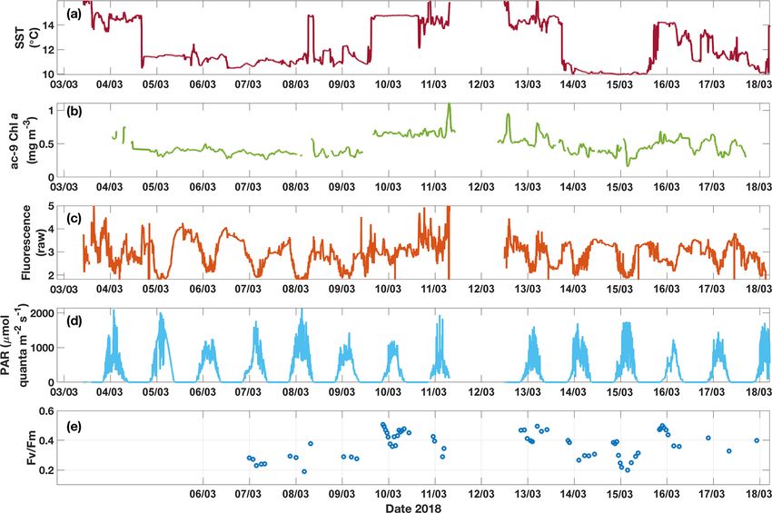
794                                   C. Schallenberg et al.: Diel quenching of Southern Ocean phytoplankton fluorescence

ment of photosynthetic competency in time and space is a                Active fluorometers such as a fast repetition rate fluorome-
crucial requirement for improved estimates and models of             ter (FRRf) exploit the complementary nature of the three pos-
oceanic primary productivity. This is especially true for areas      sible pathways of absorbed light energy. Triggering and de-
where iron (Fe) limitation is prevalent, such as the Southern        tecting changes in ChlF in the dark-regulated state (i.e. when
Ocean (Boyd et al., 2007; Moore et al., 2013). Fe-induced            NPQ is relaxed and does not quench ChlF), allows deriva-
variations in primary productivity in this region have been          tion of the commonly used parameter Fv /Fm . Fv /Fm , often
shown to arise from physiological drivers of photosynthesis          referred to as the maximum quantum yield of PSII, is a mea-
that are currently poorly represented in models of productiv-        sure of the maximum fraction of absorbed light energy that
ity (Hiscock et al., 2008). The Southern Ocean is of partic-         can be used for primary charge separation in RCII. Strong
ular interest because of its large influence on the global car-      links have been established between phytoplankton Fe status
bon cycle, which is directly linked to photosynthetic perfor-        and Fv /Fm . As Fe becomes more and more limiting, Fv /Fm
mance of the resident phytoplankton (Martínez-García et al.,         decreases (Geider et al., 1993; Greene et al., 1992). Further-
2014; Sigman and Boyle, 2000). While photosynthetic per-             more, benchtop FRRf instruments can quantify the induction
formance can readily be measured on small scales, i.e. dur-          of NPQ in response to increases in absorbed light energy, and
ing ship-based surveys conducting incubations for estimates          recent studies have found a strong link between the capacity
of primary productivity, assessment of photosynthetic com-           to induce NPQ and the Fe limitation status of phytoplankton
petency on larger scales remains challenging. Fluorescence           (Alderkamp et al., 2012; Schuback et al., 2015; Schuback
emitted by phytoplankton upon absorption of light is a signal        and Tortell, 2019).
that holds great promise in this respect, as it stems directly          The term “non-photochemical quenching” is a blanket
from the photosynthetic apparatus of phytoplankton and can           term for a number of processes and parameterizations, with
be measured by instruments mounted on drifters, floats, glid-        whole books dedicated to its many manifestations (e.g.
ers and even satellites (Letelier et al., 1997; Behrenfeld et al.,   Demmig-Adams et al., 2014). At its core, it is a photopro-
2009; Huot et al., 2013; Morrison, 2003; Schallenberg et al.,        tective mechanism that safely removes excess excitation en-
2008). Indeed, the signal has been shown to hold the poten-          ergy from the light-harvesting system of photosynthesizers
tial for providing information on the physiological state of         (Müller et al., 2001). It can be assessed in many ways, the
phytoplankton (Letelier et al., 1997; Behrenfeld et al., 2009;       most clearly defined ones are measured with active fluorom-
Morrison and Goodwin, 2010; Schallenberg et al., 2008).              eters such as FRRf, which allows for measurements in both
   Chlorophyll a fluorescence (ChlF) is one of three path-           the dark- and light-regulated state. Common parameteriza-
ways that light energy can take once absorbed by the light-          tions of NPQ include the Stern–Volmer (SV) and normal-
harvesting antenna of photosystem II (PSII) of a photosyn-           ized Stern–Volmer (NSV) parameterizations, but a myriad of
thetic organism. The other two possible pathways are pho-            other definitions are in use (e.g. Rohacek, 2002). In a less
tochemistry (i.e. primary charge separation in reaction cen-         strictly defined manner, NPQ can also be detected in mea-
tre II, RCII) and heat dissipation. Heat dissipation of ab-          surements that are made with what we will call “standard
sorbed light energy can be upregulated in situations where           fluorometers” (SF) in this paper, i.e. fluorometers conven-
light energy is absorbed in excess of photosynthetic ca-             tionally employed on floats, gliders, moorings and ships, to
pacity, which has the potential to damage the photosyn-              estimate ambient chlorophyll a concentrations as a proxy for
thetic apparatus. As the three possible pathways of absorbed         phytoplankton biomass (e.g. Roesler et al., 2017). Here, NPQ
energy are complementary, an upregulation of heat dissi-             can take the form of depressed fluorescence in the middle of
pation will quench the ChlF signal, which is known as                the day relative to the night, or it can manifest as a depression
non-photochemical quenching (NPQ) (Horton et al., 1996;              of fluorescence towards the ocean surface in daytime fluores-
Krause and Weis, 1984; Müller et al., 2001).                         cence profiles (Biermann et al., 2015; Grenier et al., 2015;
   At midday, NPQ can depress the ChlF signal by up to               Xing et al., 2012, 2018). Standard fluorometers are deployed
90 % (Falkowski et al., 2017). This affects daytime ChlF data        ubiquitously in the oceans and can be operated remotely; the
from ships, satellites, bio-optical floats and gliders, the lat-     prospect of harnessing physiological information contained
est and rapidly growing additions to the oceanographic tool-         in the NPQ signal they detect is thus tantalizing. Given the
box (Biermann et al., 2015; Grenier et al., 2015; Xing et            link between NPQ – as estimated with active fluorometers –
al., 2012, 2018). Sensitivity of NPQ to the light acclimation        and the Fe limitation status of phytoplankton (Alderkamp et
state of phytoplankton has been demonstrated (Milligan et            al., 2012; Schuback et al., 2015; Schuback and Tortell, 2019),
al., 2012; O’Malley et al., 2014), and other drivers of NPQ,         we investigated whether the NPQ signal detected by a stan-
including nutrient status and species composition, have also         dard fluorometer can also be interpreted with respect to the
been suggested (e.g. Kropuenske et al., 2009; Schallenberg et        Fe limitation status of the resident phytoplankton commu-
al., 2008; Schuback et al., 2015). An empirical relationship         nity.
between sea surface temperature and NPQ in the Southern                 The two main objectives of this study are as follows:
Ocean has been described (Browning et al., 2014), but the            (i) link NPQ capacity as measured with a FRRf to NPQ mea-
underlying controls are not fully understood.                        sured with a standard fluorometer and (ii) link the NPQ sig-

Biogeosciences, 17, 793–812, 2020                                                          www.biogeosciences.net/17/793/2020/
C. Schallenberg et al.: Diel quenching of Southern Ocean phytoplankton fluorescence 795
2 Methods
2.1 Oceanographic setting and sampling
A research voyage to the Southern Ocean Time Series
(SOTS) mooring site near 140◦ E and 47◦ S took place from 3
to 20 March 2018 aboard the RV Investigator. The SOTS site
lies in the SAZ southwest of Tasmania, an area of consider-
able mesoscale and sub-mesoscale variability (Shadwick et
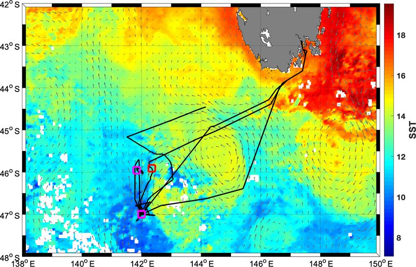
al., 2015; Weeding and Trull, 2014). During occupation of
the area, a remnant eddy with sea surface temperatures (SST)
> 14 ◦ C was just east of the SOTS site and was visited mul-
tiple times by the ship (Fig. 1).
Figure 1. Average sea surface temperature (SST) for March 2018 The ship’s underway seawater supply, which had an intake
from the MODIS-Aqua satellite, overlaid with geostrophic currents in the ship’s drop keel (water depth ∼ 7 m), was equipped
for 16 March 2018 (grey arrows) and the cruise track (black line), with a WETStar fluorometer (Wetlabs, Inc., Philomath, Ore-
as well as CTD locations in the cold water mass (purple squares) gon, USA) that measured ChlF at 695 nm (excitation at
and in the warm water mass (red square). 460 nm) continuously throughout the voyage. Travel time
through the ship’s plumbing from intake to the fluorome-
ter was between 1 and 2 min. The underway seawater line
nals from both to the Fe limitation status of the resident phy- also supplied water to a WETLabs absorption and attenua-
toplankton community. The first objective accounts for the tion metre (ac-9) in flow-through mode (see below). At regu-
fact that measurements with an FRRf are made under very lar intervals, the underway seawater supply was sampled for
controlled conditions, while the fluorescence detected with a pigment analysis by high-performance liquid chromatogra-
standard fluorometer is measured under ambient conditions phy (HPLC), particulate absorption spectra following the fil-
that can be highly variable due to differences in incident sun- ter pad approach (Mitchell, 1990), chlorophyll a concentra-
light, in the rate of change in illumination (e.g. due to pass- tion analysed fluorometrically (Chl a) and for fluorescence
ing clouds) and in the mixing depth, which also affects light light curves measured with an FRRf (more details on the
history and acclimation. We further note that there is a ship- respective methods below). Oceanic profiles (conductivity,
specific period of “dark-acclimation” prior to measurement temperature, depth, hereafter CTD) were collected at 6 sta-
if the standard fluorometer is installed on a ship’s underway tions using Sea-Bird SBE 9plus instrumentation, with asso-
seawater line, yielding an acclimation status of the phyto- ciated sampling conducted from a 36-bottle rosette equipped
plankton that is neither fully dark-regulated nor fully light- with 12 L Niskin bottles. Onboard measurements of oxygen
regulated, since some NPQ components can be reversed on and salinity on discrete samples from the Niskin bottles were
the order of minutes and even seconds (Müller et al., 2001). used to calibrate CTD sensors. Samples for macronutrients
In order to investigate our research objectives, we un- (NOx (sum of nitrate and nitrite), silicate, phosphate) were
dertook the following measurements and experiments on a also drawn from Niskin bottles and analysed onboard with a
voyage to the Subantarctic Zone (SAZ) south of Australia: Seal AA3 segmented flow instrument following the methods
(1) deck-board incubation experiments under controlled Fe of Rees et al. (2019).
conditions to confirm the link between Fe limitation and
NPQ capacity, as measured with an FRRf, in the resident
phytoplankton. (2) FRRf measurements on samples from the 2.2 Incubation experiments
underway seawater line, yielding estimates of Fv /Fm and
NPQ capacity that could be related to the Fe limitation sta- At three stations, all located in close vicinity to 47◦ S, 142◦ E,
tus of the phytoplankton. This step revealed that two distinct either a trace-metal-clean rosette system (TMR) or a trace-
water masses had been repeatedly sampled by the ship, with metal-clean pumped “fish” (i.e. a submerged body towed
significantly different Fv /Fm , indicating differences in their abeam of the ship and outside the ship wake with an intake
Fe limitation status. (3) NPQ estimated from the standard at 3–5 m depth) were deployed in order to retrieve samples
fluorometer on the underway seawater line was linked to the uncontaminated by trace metals. For each of the three incu-
different water masses and thus to Fe limitation status, as bation experiments, one initial HPLC sample was drawn and
well as to Fv /Fm and NPQ capacity measured with an FRRf. four acid-washed polycarbonate bottles (250 mL each) were
filled with unfiltered seawater from the mixed-layer and in-
cubated in a deck incubator that was continuously supplied
with surface seawater for temperature control. Light levels
were controlled with mesh bags placed around the bottles
www.biogeosciences.net/17/793/2020/ Biogeosciences, 17, 793–812, 2020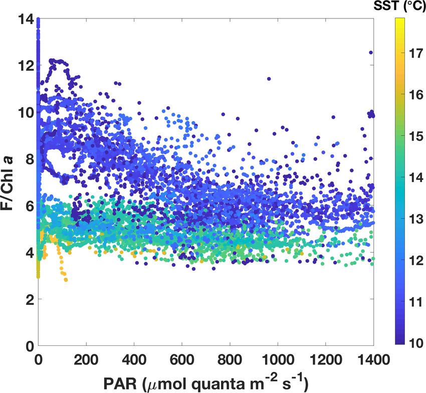
796                                   C. Schallenberg et al.: Diel quenching of Southern Ocean phytoplankton fluorescence

Table 1. Details of incubation experiments.

      Experiment    Date             Sampling time    Sampling     SST        Light level    Duration   Starting Chl a    Initial
      no.           (UTC)                   (UTC)     method       (◦ C)   (% of surface)         (h)   concentration    Fv /Fm
                                                                                                            (mg m−3 )
      1             6 Mar 2018                20:30   TMR (35 m)   10.7               67           53            0.35       0.33
      2             8 Mar 2018                18:40   Fish         11.2               67           55            0.30       0.32
      3             13 Mar 2018               22:30   Fish         10.5               25         51.5            0.37       0.34

(see Table 1). Each experiment consisted of the following           for ∼ 1 h prior to each fluorescence light curve measure-
four treatments (final concentrations indicated):                   ment to ensure relaxation of fast-relaxing NPQ as well as
                                                                    some (but likely not all) slow-relaxing NPQ. Measurement
  – 20 nM desferrioxamine B (DFB), a strong iron chelator,          of each fluorescence light curve took 24 min and was com-
                                                                    prised of eight light steps of increasing intensity (see Fig. S2
  – control (no additions)
                                                                    for details). Fluorescence light curves were optimized to
  – 0.2 nM Fe (added as FeCl3 dissolved in acidified Milli-         yield estimates of NPQ capacity at light intensities of ei-
    Q water),                                                       ther 750 µmol quanta m−2 s−1 (for samples from the under-
                                                                    way seawater system) or 1000 µmol quanta m−2 s−1 (incu-
  – 2 nM Fe (added as FeCl3 dissolved in acidified Milli-Q          bation samples). These high light intensities were chosen
    water).                                                         based on experimentation earlier in the voyage and repre-
                                                                    sent a balance such that a curve could still be fitted to the
Incubations were run for ∼ 51.5–55 h (see Table 1), and at          fluorescence induction data, while maximizing the NPQ sig-
the end of the experiments each polycarbonate bottle was            nal. Since maximum NPQ capacity was our main focus, we
sub-sampled for an FRRf measurement (see below). Fluo-              chose an experimental design that struck a balance between
rescence parameters are sensitive to the light history expe-        (i) ensuring a good fit at the maximum light intensity, (ii) in-
rienced by the phytoplankton, so the time of day at which           creasing light levels slowly enough to allow the cells to reach
measurements are made can change results. In order to make          steady-state quenching (thus choosing longer time steps at
all four treatments comparable to each other, they had to be        the more stressful high light intensities), and (iii) keeping the
measured as closely in time as possible, hence only one repli-      fluorescence light curves as short as possible so that the four
cate per treatment was prepared, allowing us to complete one        treatments in each incubation experiment could be measured
round of FRRf measurements in less than 2 h. The duration           within the smallest time frame possible (< 2 h) in recognition
of the incubations was chosen to allow an adequate physio-          of the sensitivity of fluorescence parameters to light history
logical response time (see Fig. S1 in the Supplement for the        and time of day.
time course of experiment 1, indicating that results were con-         Three measured fluorescence signals, Fo , Fm and Fm0 were
sistent between 29 and 52 h sampling points but more pro-           used to calculate fluorescence parameters, following Ro-
nounced after 52 h).                                                hacek (2002). Fo and Fm refer to minimum and maximum
                                                                    fluorescence in the dark-acclimated state, while Fm0 is the
2.3   Photosynthetic competency: FRRf measurements                  maximum fluorescence in the light-regulated state, in this
                                                                    case measured at the highest light level of the respective flu-
Photosystem II (PSII) variable ChlF was measured on a               orescence light curve.
fast repetition rate fluorometer (FRRf, Chelsea Technolo-              The maximum quantum yield of PSII, Fv /Fm , was esti-
gies Group FastOcean Sensor fitted with an Act2 laboratory          mated from fluorescence measurements during the dark step
system) using the factory-supplied Act2Run software. All            of the fluorescence light curve as follows:
measurements were made in a temperature-controlled room
that was kept at the ambient SST temperature (10–14 ◦ C).           Fv   Fm − Fo
                                                                       =         .                                                  (1)
Prior to each measurement, a blank was prepared by filter-          Fm     Fm
ing a small aliquot of sample through a 0.2 µm syringe fil-
                                                                    There are a number of different NPQ formulations available
ter and was subsequently subtracted from all measured fluo-
                                                                    in the literature (e.g. see Rohacek, 2002), each with their re-
rescence signals. The excitation wavelength of the FRRf’s
                                                                    spective advantages and disadvantages. We chose to focus on
light-emitting diodes (LEDs) was 450 nm, and the instru-
                                                                    two parameterizations, i.e. Stern–Volmer (NPQSV ) and the
ment was used in single turnover mode, with a saturation
                                                                    normalized Stern–Volmer NPQ (NPQNSV ):
phase comprised of 100 flashlets on a 2 µs pitch and a relax-
ation phase comprised of 40 flashlets on a 60 µs pitch. Sam-                    Fm − Fm0
ples were low-light acclimated (at 2–5 µmol quanta m−2 s−1 )        NPQSV =              ,                                          (2)
                                                                                  Fm0

Biogeosciences, 17, 793–812, 2020                                                            www.biogeosciences.net/17/793/2020/
C. Schallenberg et al.: Diel quenching of Southern Ocean phytoplankton fluorescence 797
Fo0 2.4.3 Fluorometric measurement of chlorophyll
NPQNSV = , (3)
Fv0
Samples for fluorometric Chl a analyses (2 L) were filtered
with Fo0 calculated following Oxborough and Baker (1997): onto 25 mm glass fibre filters (Whatman, GF/F) and immedi-
ately frozen at −80 ◦ C. Within 3 weeks of sampling, all fil-
Fo
Fo0 = , (4) ters were extracted with 10 mL of 90 % acetone at −20 ◦ C for
Fv
Fm + FFo0 24 h. Fluorescence was measured on a Turner Trilogy Labo-
m
ratory Fluorometer and converted to Chl a following the acid
and ratio method (Holm-Hansen et al., 1965). The fluorometer
had been calibrated with a spectrophotometrically measured
Fv0 = Fm0 − Fo0 . (5) dilution series of Chl a (Jeffrey and Humphrey, 1975).
Fluorometric Chl a showed excellent agreement with
Both parameters were estimated at the respective maximum Chl a measured using the HPLC method, albeit with an off-
light levels of the fluorescence light curves (i.e. 750 and set and a slight decrease in the slope relative to the 1 : 1
1000 µmol quanta m−2 s−1 for underway and incubation sam- line (Fig. S3). In order to bring the Chl a measured fluo-
ples, respectively) and should thus be regarded as a NPQ “ca- rometrically in line with the more precise HPLC measure-
pacity” that can be achieved under given nutrient availabili- ment (e.g. Trees et al., 1985), all fluorometric Chl a es-
ties and light histories of the phytoplankton assemblage (see timates were corrected using the slope and intercept from
Schuback and Tortell, 2019). The light levels at which the the regression of HPLC Chl a against fluorometric Chl a
NPQ parameters were measured are indicated in parentheses (ChlHPLC = ChlF ·0.879−0.052; r 2 = 0.97; n = 15; standard
in the respective figures; see also Table 2 for a summary of error of the estimate = 0.029 mg m−3 ). All Chl a estimates
fluorescence parameters discussed in this paper. could thus be combined for calibration of the ac-9 absorp-
tion line height approach (see below).
2.4 Phytoplankton pigments and absorption
2.4.4 Phytoplankton absorption (filter pad)
2.4.1 HPLC analyses
Sample volumes of 3–4 L were filtered through a 25 mm
Sample volumes of 3–4 L were filtered through a 25 mm
glass fibre filter (Whatman GF/F), and the filter was then
glass fibre filter (Whatman GF/F), blotted dry and stored at
stored flat at −80 ◦ C until analysis. Optical density spectra
−80 ◦ C until analysis. Samples were extracted over 15–18 h
for total particulate matter were obtained using a Cintra 404
in an acetone solution before analysis by high-performance
UV/VIS dual-beam spectrophotometer equipped with an in-
liquid chromatography (HPLC) using a C8 column and bi-
tegrating sphere. Quartz glass plates were used to hold the
nary gradient system with an elevated column temperature
sample and blank filters against the integrating sphere. The
following the method of Clementson (2013). Pigments were
optical density of the total particulate matter of each sam-
identified by retention time and absorption spectrum from a
ple was obtained using a blank filter as a reference (from
photodiode array (PDA) detector, and concentrations of pig-
the same batch number as the sample filters) wetted with fil-
ments were determined from commercial and international
tered seawater (0.2 µm) and scanned from 200 to 900 nm with
standards (Sigma, USA; DHI, Denmark).
a spectral resolution of 1.3 nm. Following the scan for total
2.4.2 Diagnostic pigment indices particulate matter, the sample filter was returned to the origi-
nal filtering units, and any pigmented material was extracted
The results from HPLC analyses were used to derive diag- using the method of Kishino et al. (1985). Blank reference fil-
nostic pigment (DP) indices following Barlow et al. (2008), ters were treated in the same manner. The filters were rinsed
which give an indication of the phytoplankton community with filtered seawater and then re-scanned to determine the
composition in terms of three functional groups: diatoms, optical density of the detrital or non-algal matter. An estimate
flagellates and prokaryotes. The DP index and resulting func- of the optical density due to phytoplankton was obtained as
tional groups are defined based on seven biomarker pigments the difference between the optical density of the total partic-
as follows: ulate matter and the detrital or non-algal matter. The optical
DP = (alloxanthin (Allo) + 190 -hexanoyloxyfucoxanthin density scans were converted to absorption spectra by first
(Hex-fuco) + 190 -butanoyloxyfucoxanthin (But-fuco) + fu- normalizing the scans to zero at 750 nm and then correct-
coxanthin (Fuco) + zeaxanthin (Zea) + chlorophyll b (Chl- ing for the path length amplification using the coefficients of
b) + peridinin (Perid)), Mitchell (1990).
Diatoms = Fuco/DP,
Flagellates = (Allo + Hex-fuco + But-fuco + Chl b)/DP,
Prokaryotes = Zea/DP.
www.biogeosciences.net/17/793/2020/ Biogeosciences, 17, 793–812, 2020798 C. Schallenberg et al.: Diel quenching of Southern Ocean phytoplankton fluorescence
Table 2. List of fluorescence-related parameters derived and discussed.
Parameter Units Method
σPSII Functional absorption cross nm2 RC−1 FRRf single turnover protocol during dark-
section of PSII regulated state
F Fluorescence Arbitrary Measured with a standard fluorometer with minimal
or no dark-acclimation period
Fmin Minimum fluorescence in Arbitrary Measured with a standard fluorometer, with mini-
the day (at high light) mal or no dark-acclimation
Fmax Maximum fluorescence in Arbitrary Measured with an standard fluorometer, with mini-
the day (at low light) mal or no dark-acclimation
Fv /Fm Maximum quantum yield No units FRRf single turnover protocol during dark-
of PSII regulated state, calculated as (Fm − Fo )/Fm
NPQ Non-photochemical No units Term comprised of a number of non-photochemical
quenching quenching processes that decrease fluorescence at
0 relative to
supersaturating light intensities (e.g. Fm
Fm and Fmin relative to Fmax )
NPQNSV (750), NPQNSV (1000) Normalized Stern– No units FRRf single turnover protocol during light-
Volmer NPQ at light regulated state, i.e. Eq. (3)
intensities of 750 and
1000 µmol quanta m−2 s−1
NPQSV (750), NPQSV (1000) Stern–Volmer NPQ at No units FRRf single turnover protocol during light-
light intensities of 750 and regulated state, i.e. Eq. (2)
1000 µmol quanta m−2 s−1
NPQSF NPQ analogous to Stern– No units Measured with a standard fluorometer with mini-
Volmer NPQ mal or no dark-acclimation, calculated as (Fmax −
Fmin )/Fmin
2.4.5 Particulate absorption (ac-9) of repeat measurements on Milli-Q water in the laboratory
prior to the voyage (2–7 min each, then the average taken
A WETLabs ac-9 instrument with 25 cm flow tubes was em- for each measurement) indicated that the precision of these
ployed in underway mode on the underway seawater line of three channels ranged from 0.0023 to 0.0028 m−1 (2.3 %–
the RV Investigator. The instrument was immersed in the 2.9 %) when expressed in terms of the standard deviation of
upright position in a flow-through water bath for tempera- measurements (n = 8). The absolute range, determined as the
ture control, and the flow tubes were shielded from ambi- difference between the maximum and minimum value of the
ent light. Flow was upwards through the tubes and trickled measurements, was 0.0059–0.0071 m−1 (5.9 %–7.4 %).
from there into the water bath, where an overflow valve con- Bubbles in the flow tubes were a common problem on the
trolled the water level. About two-thirds of the instrument voyage and were dealt with by applying a thorough clean-
was immersed, with the upper part exposed to the atmo- ing routine as well as smoothing of the time series during
sphere. Internal instrument temperature was monitored ev- processing (see Supplement for details). Particulate absorp-
ery few hours and fluctuated between 21 and 26 ◦ C. The tion was calculated by subtracting interpolated filtered mea-
inflow was manually switched between unfiltered and fil- surements (i.e. dissolved absorption) from unfiltered mea-
tered seawater (0.8/0.2 µm; AcroPak™ 1500 capsule filter surements (total absorption) at each wavelength (Slade et
with Supor® membrane), with filtered measurements last- al., 2010). The particulate absorption line height at 676 nm
ing ∼ 10 min and conducted every ∼ 2 h. The flow rate was (LH(676), m−1 ) was then calculated following Roesler and
1–1.5 L min−1 for unfiltered seawater and not lower than Barnard (2013), subtracting a baseline based on absorption
0.5 L min−1 for filtered seawater. The filter was exchanged measurements at 650 and 715 nm. This LH(676) was cali-
for a new one after 10 d. brated against discrete Chl a (Chl a from fluorometric and
Because we were only interested in the absorption line HPLC measurements combined; see above) and also against
height at 676 nm, only the red absorption channels of the phytoplankton absorption as determined with the filter pad
ac-9 (λ = 650, 676 and 715 nm) were processed. Analysis method (see Supplement).
Biogeosciences, 17, 793–812, 2020 www.biogeosciences.net/17/793/2020/C. Schallenberg et al.: Diel quenching of Southern Ocean phytoplankton fluorescence 799
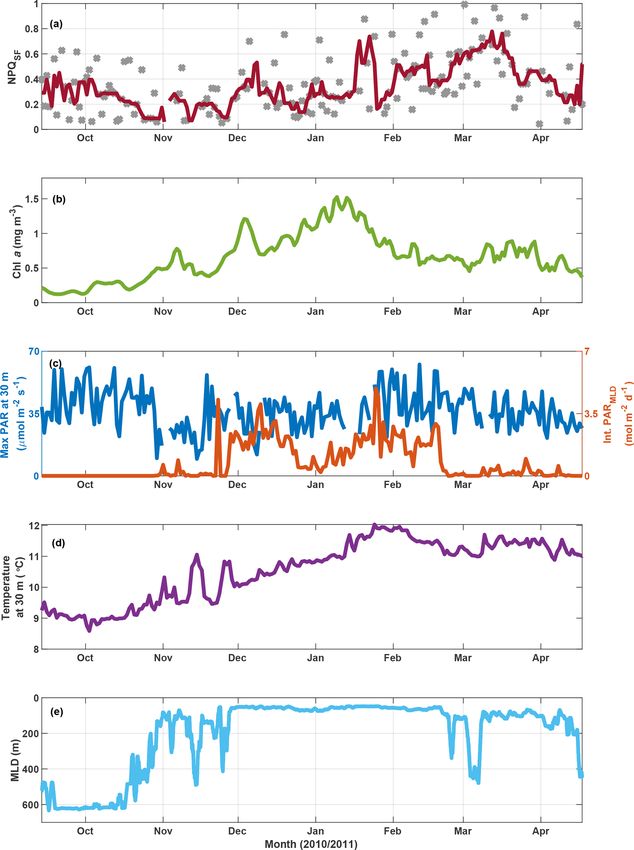
2.5 Simulated in situ measurements of and mixed-layer depth (MLD) was calculated based on a
size-fractionated primary production temperature difference of 0.3 ◦ C relative to the 30 m mea-
surement. Only data with a quality flag < 2 were used, and
Photosynthetic production of organic matter was measured the fluorescence sensor had been calibrated using factory-
twice during the voyage (7 and 18 March 2018; both times supplied dark values and scale factors (Schallenberg et al.,
with water from SST < 11.5 ◦ C) by the 14-carbon (14 C) 2019). Fluorescence-based WETLabs ECO sensors have
tracer method. Algal carbon fixation was measured on sam- been shown to overestimate Chl a in the Southern Ocean by
ples collected pre-dawn from trace-metal-clean Niskin bot- up to a factor of 7 compared to pigment samples, with a fac-
tles deployed on a TMR from three or four depths: 35, tor of ∼ 4 overestimation reported for the Indian sector of the
50, (70 m for the 18 March incubation) and 100 m. Sam- Southern Ocean (Roesler et al., 2017). We have thus divided
pling depths were determined from in situ irradiance depth the fluorescence output from the FLNTUS sensor by 4 when
profiles obtained during midday CTD casts on the day Chl a concentration as a proxy of phytoplankton biomass was
prior to the collection. Samples were dispensed into 300 mL the entity of interest, consistent with previous approaches to
acid-washed polycarbonate bottles and spiked with 16 µCi fluorescence data from the SAZ (e.g. Eriksen et al., 2018).
of sodium 14 C-bicarbonate (NaH14 CO3 ; specific activity However, the fluorescence data were also used to estimate
1.85 GBq mmol−1 ; PerkinElmer). Following the addition of NPQ over the daily cycle, and for this exercise fluorescence
14 C, samples were incubated for 24 h in neutral density mesh was neither divided by 4 nor in any other way normalized to
bags in a deck-board incubator. The temperature of the incu- biomass.
bator was controlled by a continuous supply of surface sea- NPQ from the FLNTUS fluorometer was estimated analo-
water. Six samples (five light and one dark bottle per irradi- gously to the Stern–Volmer parameterization:
ance) were incubated under natural sunlight at six light in- Fmax − Fmin
tensities (from 67 % to 0.2 % of incident irradiance), which NPQSF = , (6)
Fmin
were adjusted by varying the layers of neutral density mesh.
Light attenuation was measured with a Biospherical Instru- where NPQSF stands for NPQ measured with a standard
ments QSL2101 Quantum Scalar PAR (Photosynthetically fluorometer and Fmax and Fmin are the maximum and min-
Available Radiation) Sensor. Carbon fixation based on ra- imum fluorescence measurements made with said fluorome-
dioisotope measurements and 24 h incubations are reported ter in a day, with the following restrictions: the daily fluores-
to approximate net primary production (Laws, 1991). cence and PAR data were first smoothed with a loess (local
Upon completion of the 24 h incubation, four replicate regression using weighted linear least squares and a second-
samples were filtered in series through 0.2, 2.0 and 20 µm degree polynomial model) filter, and NPQSF was only esti-
polycarbonate filters (Poretics) separated by 200 µm nylon mated if the minimum fluorescence was within 2 h of max-
mesh, and two samples were filtered through 0.2 µm filters imum PAR. The parameter Fmax designates the maximum
(a total community “light” control and a total community smoothed fluorescence between 05:00 and 12:00 LT on a
“dark” control). Data for the dark-corrected size-fractionated given day. This was preferable to using Fmax from night-time
samples are reported here. Filters were rinsed with 0.2 µm fil- because it decreases the time gap between the two fluores-
tered seawater, acidified to volatilize any remaining inorganic cence measurements and thus the likelihood of Fmax varying
carbon (Boyd and Harrison, 1999) and collected in 20 mL due to fluctuations in Chl a concentrations is reduced. Fur-
glass scintillation vials (Wheaton) into which 10 mL of liquid thermore, this approach corresponds to analyses carried out
scintillation cocktail (UltimaGold, PerkinElmer) was added. on the underway fluorescence data from the SOTS voyage,
Samples were subsequently analysed by liquid scintillation as discussed below. Note that NPQSF is a “realized” NPQ at
counting (PerkinElmer Tri-Carb 2910 TR). Water-column- incident light, in contrast to the NPQ capacity estimated with
integrated carbon assimilation rates were calculated using the the FRRf.
trapezoid rule with the shallowest value extended to 0 m and
the deepest extrapolated to a value of zero at 200 m. 3 Results and discussion
2.6 Mooring data 3.1 Incubation experiments: sensitivity of ChlF
parameters to Fe status
We show SOTS mooring data from the Pulse-7 deployment
in 2010–2011. The mooring was equipped with a number The incubation experiments were designed with the goals
of instruments, including a downward-looking WETLabs of (1) testing whether the resident phytoplankton were Fe-
ECO FLNTUS fluorometer with a “bio-wiper” at 30 m and limited and (2) investigating how NPQ capacity and Fv /Fm ,
a wiped ECO PAR sensor at the same depth. Seawater tem- as derived from FRRf measurements, respond to changes
perature was measured at 15 discrete depths with Vemco in Fe status. All three incubations were carried out with
Minilog Classic sensors (except for the shallowest sensor source waters colder than 11.5 ◦ C (Table 1), i.e. with wa-
at 30 m, which was a Sea-Bird Electronics SBE16plusV2), ters from the colder water mass as evident in Fig. 1, and
www.biogeosciences.net/17/793/2020/ Biogeosciences, 17, 793–812, 2020800 C. Schallenberg et al.: Diel quenching of Southern Ocean phytoplankton fluorescence
Figure 2. FRRf results after ∼ 53 h for the three pooled incubation experiments. The respective treatments are indicated on the x axes
(2 and 0.2 nM Fe additions were pooled into +Fe), and measured parameters are on the y axes. NPQ capacity was estimated at
1000 µmol quanta m−2 s−1 after 24 min exposure to increasing actinic light intensities (see Fig. S2 for details of the fluorescence light
curves). Box plots show the sample medians in red, with the blue boxes indicating the 25th and 75th percentiles; whiskers extend to the most
extreme data points. All +Fe treatments were significantly different from the respective DFB treatments (Wilcoxon rank-sum test, p < 0.05),
and all +Fe treatments, except for σPSII , were also significantly different from the respective control treatments.
the respective pigment compositions of the resident phyto- increased capacity and need to dissipate excess excitation en-
plankton were very similar (Fig. S4), indicating a dominance ergy as NPQ.
of haptophytes, with some diatoms and chrysophytes also For all parameters except σPSII , the results for the +Fe
present. The pooled data from the experiments show un- treatment were significantly different from the respective
equivocally that Fe addition increased the maximum quan- control (Wilcoxon rank-sum test, p < 0.05), indicating that
tum yield of PSII, Fv /Fm , as has been observed previously in phytoplankton in the sampled water mass, i.e. the cold wa-
HNLC regions (e.g. Boyd and Abraham, 2001; Kolber et al., ters < 11.5 ◦ C, were Fe-limited. This view is further sup-
1994). The NPQ capacity, measured as both NPQSV (1000) ported by the low initial Fv /Fm observed for all experiments
and NPQNSV (1000), decreased with Fe addition (Fig. 2), (∼ 0.33, Table 1); a fully dark-regulated Fv /Fm in this range
most likely due to increased capacity for using absorbed is a widely accepted indicator of Fe limitation in HNLC wa-
light energy for photochemistry. The functional absorption ters (Boyd and Abraham, 2001; Kolber et al., 1994; Suggett
cross section of PSII, σPSII , also decreased with Fe addi- et al., 2009).
tion, as has been observed previously (Kolber et al., 1994; The changes in NPQ capacity were diametrically oppo-
Schuback et al., 2015; Schuback and Tortell, 2019). Overall, site to the changes in Fv /Fm with respect to Fe status: as Fe
σPSII were very large in all treatments (∼ 10–12 nm2 RC−1 ), stress increased, so did the capacity for NPQ. Similar NPQ
as has been observed previously for low Fe-adapted South- responses to Fe status have been observed previously in con-
ern Ocean phytoplankton (Strzepek et al., 2012, 2019). The trolled experiments both in the laboratory and with natural
addition of DFB, a strong organic ligand (siderophore) that phytoplankton communities from Fe-limited ocean regions
decreases Fe availability to phytoplankton, had the opposite (e.g. Alderkamp et al., 2012; Petrou et al., 2014; Schuback
effect to Fe addition for all parameters. The phytoplankton et al., 2015; Schuback and Tortell, 2019). While some of
thus showed a clear response to changes in Fe status, which these studies reported NPQSV , others estimated NPQNSV ,
affected their ability to process absorbed light energy, evident hence we decided to investigate the Fe effect on both. Non-
in a lower maximum quantum yield of PSII, Fv /Fm , and an photochemical quenching affects all fluorescence levels and
is most easily quantified using the Stern–Volmer parameter-
Biogeosciences, 17, 793–812, 2020 www.biogeosciences.net/17/793/2020/C. Schallenberg et al.: Diel quenching of Southern Ocean phytoplankton fluorescence 801
ization, which was originally developed for higher plants.
However, this parameterization does not take into account
differences in Fv /Fm in the dark-regulated state, which can
mask differences in NPQ as only the light-induced compo-
nent is assessed, ignoring differences in basal levels of heat
dissipation. The normalized Stern–Volmer parameterization
explicitly accounts for differences in Fv /Fm , which means it
is a more appropriate parameter when samples with different
Fv /Fm are being compared, as is the case in our incubations
with different levels of Fe stress. However, it is important
to note that, mathematically, NPQNSV is inversely related to
Fv /Fm when Fo0 is calculated (see Eq. 4) rather than mea-
sured directly, as is the case in our study:
Fo Fv
NPQNSV = / . (7)
Fm0 Fm
Figure 3. FRRf results from underway samples (n = 66). NPQ ca-
This inverse mathematical relationship, in conjunction with pacity at a light intensity of 750 µmol quanta m−2 s−1 is plotted
the established sensitivity of Fv /Fm to Fe limitation (Boyd against Fv /Fm , with two different NPQ parameterizations used
and Abraham, 2001; Kolber et al., 1994; Suggett et al., 2009), as follows: normalized Stern–Volmer (a) and Stern–Volmer (b).
means that NPQNSV is not a truly independent parameter Colour indicates SST of the corresponding waters.
with respect to Fe status, even though the inverse relation-
ship with Fv /Fm may be physiologically relevant. Further-
more, measurement of NPQNSV requires knowledge or cal- summer (Boyd et al., 2001; Hutchins et al., 2001; Lannuzel
culation of Fo or Fo0 (Eqs. 3–5), which means it can only be et al., 2011; Sedwick et al., 1999).
measured with an active fluorometer, such as a FRRf. Con-
versely, parameters analogous to the NPQSV parameter can 3.2 Underway data: two SST regimes with different
be estimated with any fluorometer so long as a dark-regulated ChlF parameters (FRRf)
and light-regulated measurement is available.
Fluorescence measurements similar to the ones carried out
A physiological relationship between NPQ and Fe stress
on the incubations were also performed on samples taken
can be understood conceptually as a result of increased ex-
from the underway seawater line on the SOTS voyage (n =
citation pressure on the reaction centres when Fe is limiting
66). Fv /Fm ranged from 0.2 to 0.5 in the resident phyto-
(Schuback et al., 2015). Under Fe stress, there are fewer re-
plankton and showed an inverse relationship with NPQ ca-
action centres and electron transport chains per chlorophyll
pacity (Fig. 3), as was observed for the incubations. The
because electron transport chains are Fe-expensive (Behren-
trends in ChlF parameters appeared to fall into two groups
feld and Milligan, 2013). More energy is thus funnelled to
based on sea surface temperature (SST): phytoplankton in
fewer reaction centres, which causes the increase in σPSII
the colder water mass (< 11.5 ◦ C) showed lower Fv /Fm and
(Alderkamp et al., 2019; Ryan-Keogh et al., 2017; Strzepek
higher NPQ capacity, consistent with increased Fe limitation,
et al., 2012). This arrangement comes at the expense of the
compared to the phytoplankton in the warmer water mass
ability to deal with fluctuations in light; the system is “less
(> 13.5 ◦ C). Grouping the ChlF parameters based on SST il-
robust”. Iron limitation thus increases the need for rapid pho-
lustrates this point even further (Fig. 4): Fv /Fm , as well as
toprotection, which can be achieved through an increased ca-
the capacity to dissipate excess excitation energy (estimated
pacity for NPQ, as has been observed previously (Schuback
as NPQNSV and NPQSV ), was significantly different between
et al., 2015; Schuback and Tortell, 2019).
the two water masses (p
0.01, Wilcoxon rank-sum test). It
From the data presented above, we conclude that the res-
thus appears that the phytoplankton in the two SST regimes
ident phytoplankton in the colder water mass were indeed
experienced different levels of Fe stress, but before such a
Fe-limited (evident in the clear treatment response to Fe-
conclusion can be drawn, a number of confounding factors
addition, Fig. 2) and that both the NPQ capacity and Fv /Fm ,
must be discussed, including species composition, mixed-
as derived from FRRf measurements, responded to changes
layer depth and the effect of temperature on physiology.
in Fe status. While Fv /Fm increased with Fe addition, the
NPQ capacity decreased, consistent with expectations. The
observation that the colder water mass exhibited signs of Fe
limitation is also consistent with expectations, as the SAZ,
and the SOTS site in particular, has been shown to be season-
ally Fe-limited, with limitation increasing towards the end of
www.biogeosciences.net/17/793/2020/ Biogeosciences, 17, 793–812, 2020802 C. Schallenberg et al.: Diel quenching of Southern Ocean phytoplankton fluorescence
Figure 4. Comparison of FRRf data from underway samples, grouped based on SST. All parameters are significantly different between the
two respective water masses (Wilcoxon rank-sum test, p
0.01).
between the two SST regimes, the overall pattern is similar,
indicating that the phytoplankton assemblages in the two wa-
ter masses were comparable (see Figs. S5 and S6 for detailed
pigment and phytoplankton absorption results). Moreover,
these distributions among major phytoplankton groups are
consistent with the phytoplankton community composition
in the SAZ reported by Mendes et al. (2015) using similar
methods. These authors also conducted a CHEMTAX anal-
ysis of their data that suggested a dominance of haptophytes
in the SAZ, with pelagophytes, prasinophytes and diatoms
making up the majority of other taxa. A recent microscopic
analysis of fortnightly samples from a remote sampler on the
SOTS mooring at 47◦ S, 142◦ E likewise indicated that flagel-
lates were the most abundant phytoplankton group between
September and April, followed by diatoms (Eriksen et al.,
Figure 5. Mean diagnostic pigment (DP) indices calculated based
2018). The results from the DP index analysis are thus con-
on pigment ratios from HPLC analyses for samples taken from
the underway seawater supply, grouped by SST (n = 6 for SST >
sistent with previous estimates for the region and show that
13.5 ◦ C; n = 7 for SST < 11.5 ◦ C). Error bars indicate 1 standard the two SST regimes were broadly similar with respect to
deviation. See Sect. 2.4.2 for calculation of the DP index. phytoplankton community composition.
3.2.2 Mixed-layer depths and average light field
3.2.1 Phytoplankton pigments and community
composition in the two SST regimes The depth of the mixed layer can have a profound impact on
NPQ capacity, as phytoplankton acclimate to their light expo-
The diagnostic pigment (DP) index, calculated from HPLC sure. Deeper mixed layers, resulting in stronger fluctuations
pigment analyses, provides a simple though not definitive in light availability, have been found to increase the NPQ
means of investigating phytoplankton community compo- capacity of phytoplankton in the field and under simulated
sition. It focusses on three major groups (diatoms, flagel- conditions in the laboratory (Browning et al., 2014; Milligan
lates and cyanobacteria) selected on the basis of their signif- et al., 2012). In our study region, the mixed-layer depth was
icance rather than their respective size ranges (Barlow et al., deepest in the warm SST regime (∼ 100 m; Fig. S7), while it
2008). Such a diagnostic index is naturally a simplification ranged between 20 and 90 m in the colder regime. The cor-
and should be treated with caution. However, the DP index responding median daily integrated PAR in the mixed layer
has been used across a number of ecological ocean regions, (for a nominal clear-sky day in March and with PAR atten-
including the SAZ and Southern Ocean, where it compared uation estimated as a function of Chl a based on Morel et
favourably to the more elaborate CHEMTAX analyses (e.g. al., 2007) was 0.13 mol m−2 d−1 for the warm SST regime,
Mendes et al., 2015). while it ranged from 0.5 to 15 mol m−2 d−1 for the cold SST
Our analysis indicates a dominance of flagellates in both regime. If the rates and magnitude of light intensity fluctu-
the warm and cold SST regimes, with diatoms and prokary- ations were the drivers for the observed differences in NPQ
otes playing a lesser role (Fig. 5). Despite some differences capacity between the two water masses, we would expect the
Biogeosciences, 17, 793–812, 2020 www.biogeosciences.net/17/793/2020/C. Schallenberg et al.: Diel quenching of Southern Ocean phytoplankton fluorescence 803
warmer water mass (with the deep mixed layer) to show in- well with those measured at the SOTS site in March 2016
creased NPQ capacity. However, the observed NPQ trend is using the same method (670 ± 25 mg C m−2 d−1 ) (Ellwood et
exactly the opposite, with higher NPQ capacity evident in the al., 2020) but are considerably lower than those measured by
colder water mass. With only one CTD station in the warmer Westwood et al. (2011) in subantarctic waters in austral sum-
SST regime, we may have under-sampled this water mass, mer (January–February 2007) when Fe concentrations are
but it is unlikely that it showed overall shallower mixed lay- higher: 1034–1627 mg C m−2 d−1 . While part of the differ-
ers than the cold-water regime. We thus conclude that the ence between our results and those of Westwood et al. (2011)
observed trend in NPQ capacity can not be explained by the may be due to methodological differences, i.e. short (2 h) ver-
mixed-layer depths encountered. sus long (24 h) 14 C incubations, we ascribe most of the dif-
ference to the seasonal cycle of Fe limitation observed pre-
3.2.3 Temperature effects on phytoplankton viously for SOTS (Boyd et al., 2001; Hutchins et al., 2001;
photophysiology Lannuzel et al., 2011; Sedwick et al., 1999). See the Supple-
ment for a full comparison of observed conditions between
It is well established that temperature has a strong effect on this study and Westwood et al. (2011).
phytoplankton growth, especially with respect to the opti- Fewer ancillary data are available for the warmer water
mal niche for a given species (e.g. Boyd et al., 2013; Davi- mass, as there were no primary productivity measurements
son, 1991; Raven and Geider, 1988). However, the maximum or Fe-addition experiments undertaken. However, macronu-
quantum yield of PSII, Fv /Fm , appears less sensitive to tem- trient data from the one CTD in that water mass indicate that
perature. Manipulative studies have reported little or no ef- the warm SST regime was not high nutrient–low chlorophyll
fect on Fv /Fm for phytoplankton grown at temperatures dif- (HNLC), as NOx was drawn down to near zero, which was
fering by 4–8 ◦ C between minimum and maximum tempera- not the case for the colder waters where NOx was always
ture (e.g. Kulk et al., 2012; Rose et al., 2009). Indeed, the well above 5 µM (Fig. S9). Phosphate concentrations were
latter study specifically investigated the synergistic effects also significantly lower in the warmer waters than the cold
of Fe and temperature on Antarctic phytoplankton. An in- waters, while silicate was depleted for both.
crease in temperature by 4 ◦ C did not result in any change The SST map in Fig. 1 indicates that the warm SST
of Fv /Fm compared to the control, but an addition of Fe in- signature near SOTS was part of a cyclonic eddy, which
creased Fv /Fm significantly – with and without an increase could be tracked back in time to even warmer waters south-
in temperature (Rose et al., 2009). We thus conclude that it is west of Tasmania based on its signature on satellite altime-
highly likely that the differences in Fv /Fm and NPQ capac- try and SST images (not shown). At the time of sampling,
ity we observed between the two SST regimes (with mean the eddy-associated water mass exhibited SSTs reaching >
SSTs of 10.8 ± 0.5 and 14.6 ± 0.7 ◦ C, respectively) were the 14 ◦ C, compared to < 12 ◦ C for the waters further west, and
result of physiological changes in the phytoplankton due to showed warmer and saltier water throughout the water col-
their nutritional (Fe) status, rather than being caused by the umn, with a salinity minimum around 34.4 (Fig. S10). Such
different ambient temperatures. a temperature–salinity signature is consistent with an origin
of the eddy-associated water mass either east or west of Tas-
3.2.4 The case for differences in physiological status in mania, with a strong influence from the Tasman Sea (Herraiz-
the two SST regimes Borreguero and Rintoul, 2011). Waters east of Tasmania have
previously been found to be Fe-replete (and low in nitrate),
The strongest indicator that the two SST regimes held phyto- with airborne dust and shelf sediments presumed to be the
plankton communities with different levels of Fe stress is the main Fe sources (Bowie et al., 2009; Lannuzel et al., 2011).
difference in Fv /Fm between the two regimes (Fig. 4). The Fv /Fm values indicative of Fe sufficiency (∼ 0.5) were also
decrease in Fv /Fm in the colder water mass corresponded to reported for the SAZ southeast of Tasmania (SST ∼ 15 ◦ C)
a large increase in Fo relative to the warm regime (Fig. S8), in late summer, along with very low nitrate and non-limiting
in line with the hypothesis that under Fe limitation damaged Fe concentrations at the surface (Hassler et al., 2014). It is
and/or disconnected light-harvesting complexes contribute to thus highly likely that the warmer water mass encountered
background fluorescence, as has been previously observed during the SOTS voyage in 2018 was Fe-replete, while the
(Behrenfeld and Milligan, 2013). The corresponding increase colder water mass was Fe-limited. The absence of dissolved
in Fm in the presumably Fe-limited water mass is also not un- Fe data leaves the Fe nutritional status of the warmer wa-
expected and has been observed in other Fe-limited regions ter mass community less than completely clear (although the
(e.g. Behrenfeld and Kolber, 1999). presence of Fv /Fm values above 0.4 suggests Fe limitation
Rates of water-column-integrated net primary productivity was unlikely since Fe status is known to be the dominant
measured in the cold SST regime also point to Fe limitation driver for Fv /Fm in the Southern Ocean, e.g. Suggett et al.,
in that water mass. Column-integrated primary production 2009). Regardless of this uncertainty, the Fe-limited status
rates ranged from 317±30 mg C m−2 d−1 (18 March 2018) to and corresponding high NPQ capacity of the cold-water com-
500 ± 104 mg C m−2 d−1 (7 March 2018). These rates agree munity is clear.
www.biogeosciences.net/17/793/2020/ Biogeosciences, 17, 793–812, 2020804 C. Schallenberg et al.: Diel quenching of Southern Ocean phytoplankton fluorescence
Figure 6. Time series for underway data from the SOTS voyage in 2018 of (a) SST, (b) Chl a from ac-9, (c) raw fluorescence, (d) above-
water PAR and (e) Fv /Fm measured on dark-acclimated discrete samples. Diel fluctuations in fluorescence are apparent, especially when
cold water was sampled. These fluctuations are not found in the corresponding Chl a time series. Note that the data gap around 12 March is
due to the ship leaving the SAZ region during that time.
3.3 Underway data: continuous measurements across 3.3.1 Physiological information in underway
the two SST regimes fluorescence: NPQ differences between the two
SST regimes
The two SST regimes were repeatedly visited by the ship dur-
ing the voyage (Fig. 6). The Chl a data from the ac-9 were
remarkably different from the fluorometer traces (compare In order to investigate NPQ as measured with the standard
Fig. 6b and c), with clear day–night fluctuations in the lat- fluorometer (Fig. 6c) in more detail, we normalized fluores-
ter that were not reflected in the ac-9 data. These fluctuations cence by Chl a as estimated by the ac-9 and plotted it against
were especially pronounced in the colder water mass, which incident daytime PAR (Fig. 7). Colour-coding by SST clearly
had overall lower Chl a concentrations than the warmer wa- shows that two NPQ regimes were at play. In the colder wa-
ters (mean Chl a = 0.38 ± 0.06 mg m−3 for SST < 11.5 ◦ C ters, F/Chl a was high at low PAR and decreased consid-
and 0.62 ± 0.11 mg m−3 for SST > 13.5 ◦ C). The daily fluo- erably as PAR increased – dynamic NPQ was high. In the
rescence minima coincided with the maxima in above-water warmer waters, F/Chl a was relatively constant across PAR
incident PAR and vice versa; i.e. fluorescence was highest values and dynamic NPQ was thus low. Note that normaliza-
during the night. Such daily fluorescence cycles are consis- tion to Chl a removes differences in the fluorescence signal
tent with non-photochemical quenching of fluorescence in that would be caused by differing Chl a concentrations in the
the daytime. water masses.
The NPQ signal from the standard fluorometer was fur-
ther investigated by formally separating the data from the
two water masses based on SST (Fig. 8). A loess filter was
applied to the respective pooled data sets (for values mea-
sured at PAR > 5 and PAR < 1000 µmol quanta m−2 s−1 ),
Biogeosciences, 17, 793–812, 2020 www.biogeosciences.net/17/793/2020/C. Schallenberg et al.: Diel quenching of Southern Ocean phytoplankton fluorescence 805
Antarctic Circumpolar Current, while subtropical gyre-type
waters, where Fe was replete and nitrogen was low, exhib-
ited subdued NPQ. Overall, they found that their NPQ pa-
rameterization showed the strongest correlation with SST,
which they interpreted to be largely caused by the relation-
ship between SST and the extent of near-surface stratifica-
tion and mixed-layer depth (Browning et al., 2014). They
also found a correlation between NPQ and Fv /Fm that was
statistically significant at the p < 0.001 confidence level but
was weaker than that with SST. It is worth pointing out that
there were significant methodological differences between
their approach and ours, as well as a much larger SST gradi-
ent in their study region (3–25 ◦ C), which likely has its own
correlation with Fe limitation while also causing differences
in species composition that can have a strong influence on
Fv /Fm (Suggett et al., 2009). Regardless of the cause in NPQ
variability, our findings reinforce the observation by Brown-
Figure 7. Underway fluorescence data normalized to Chl a plotted
ing et al. (2014) that NPQ can be highly variable due to fac-
against incident PAR above the surface. Chl a was estimated from tors other than incident PAR, implying that NPQ corrections
ac-9 data. Data points are colour-coded according to SST. that rely solely on PAR should be viewed with caution.
Overall, our results are consistent with the differences in
NPQ observed in the two SST regimes being caused by dif-
ferences in their Fe limitation status, as evidenced in the re-
and NPQSF (NPQ measured with a standard fluorometer) was spective Fv /Fm , with implications for the expected efficiency
estimated from the filtered data according to Eq. (6). The of photochemistry. Not only did we find a strong inverse
NPQSF signal in the colder, HNLC water mass was more relationship between Fv /Fm and NPQ capacities estimated
than twice as high as that in the warm SST regime, and a with an FRRf light-curve protocol, but the relationship was
similar trend was discernible even without normalization of also borne out in NPQSF measured with a standard fluoro-
the fluorescence signal to Chl a (Fig. 8). The trends in NPQ meter – an instrument type frequently used on moorings,
as evidenced in the data from the standard fluorometer are ships and autonomous measuring platforms, such as Argo
thus consistent with the NPQ capacities measured with the floats. We have thus shown that measurements from a stan-
FRRf (Fig. 4): increased dynamic NPQ (and NPQ capacity) dard fluorometer can provide useful information on phyto-
in the colder waters relative to the warm SST regime. This plankton physiology, in particular the presence of Fe stress.
result is significant as it indicates that measurements from a While the phytoplankton community in our study was dom-
standard fluorometer can be interpreted with regards to phy- inated by flagellates (Fig. 5), we expect that our results hold
toplankton physiological status. Without the control afforded across a range of phytoplankton species, as the relationship
by an FRRf, simply using a standard fluorometer and the between NPQ and Fe limitation status has been observed
daily cycle of the sun, a signal is measured (NPQSF ) that in laboratory and field studies elsewhere, including phyto-
holds profound physiological information. This should not plankton communities dominated by diatoms (Schuback et
come as a complete surprise, as it has long been recognized al., 2015; Schuback and Tortell, 2019).
that standard fluorometers are affected by NPQ, and consid-
erable research has gone into investigating how to best cor- 3.4 Case study: application of NPQSF approach to
rect for NPQ in order to retrieve more accurate profiles of mooring data
Chl a concentration (Biermann et al., 2015; Thomalla et al.,
2018; Xing et al., 2012, 2018). However, given the depen- In order to further test the utility of this interpretation of
dence of NPQ on incident irradiance, attempts to correct for fluorescence measured with a standard fluorometer, we in-
it in a “physiological” way have tended to be based on irradi- vestigated NPQSF on a time series from the SOTS mooring
ance thresholds or light history (e.g. Behrenfeld et al., 2009; (Fig. 9a). Here, NPQSF was estimated based on daily fluores-
Xing et al., 2018), while ignoring other factors affecting phy- cence measurements, after application of a smoothing filter
toplankton physiological status, such as Fe limitation. (see Sect. 3.3.1). Due to differences in the maximum PAR on
A noteworthy exemption is the study by Browning et any given day, one could argue that NPQSF should be nor-
al. (2014), which specifically investigated the variability malized by the incident PAR at Fmin , as the depression in
of NPQ along eco-physiological gradients in the Southern fluorescence is expected to be proportional to the incident
Ocean. That study showed similar trends to ours: increased light. Such a measure decreases the scatter in the time series
dynamic NPQ was associated with Fe-limited waters of the but preserves the overall trend observed in Fig. 9a (Fig. S11).
www.biogeosciences.net/17/793/2020/ Biogeosciences, 17, 793–812, 2020You can also read