THE ICT PSP METHODOLOGY FOR ENERGY SAVING MEASUREMENT A COMMON DELIVERABLE FROM PROJECTS OF ICT FOR SUSTAINABLE GROWTH IN THE RESIDENTIAL SECTOR
←
→
Page content transcription
If your browser does not render page correctly, please read the page content below

THE ICT PSP METHODOLOGY FOR
      ENERGY SAVING MEASUREMENT
                                                          -
  A COMMON DELIVERABLE FROM
 PROJECTS OF ICT FOR SUSTAINABLE
GROWTH IN THE RESIDENTIAL SECTOR

                                   (Version 2 – September 2011)

         Project co-funded by the European Commission within the ICT Policy Support Programme

                                                Dissemination Level

 PU    Public                                                                                   X

 RE    Restricted to a group specified by the consortium (including the Commission Services)

                                                                                                    1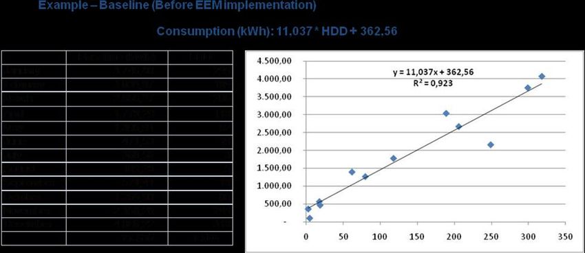
REVISION HISTORY AND STATEMENT OF ORIGINALITY

Rev    Date            Author        Organization                    Description

 1    May 2011     Günter Lohmann        IWU         Revision of chapter “Methodology for energy
                                                               efficiency measurement”

 2    July 2011    Gregor Heilmann     empirica         Restructuring of version 1 (Introduction)

 3    July 2011      Ulrike Hacke        IWU         Revision of chapter “Methodology for impact
                                                                     assessment”

                                                          Restructuring, formatting of chapter
                                                          “Methodology for energy efficiency
                                                                    measurement”

 4     August      Simon Robinson      empirica         Integration of impact assessment and
        2011                                        methodology for measurement of energy savings

 5 September         Ulrike Hacke        IWU                           Final edit
      2011

 6 September       Gregor Heilmann     empirica                Final edit and submission
      2011

Statement of originality

This deliverable contains original unpublished work except where clearly indicated otherwise.
Acknowledgement of previously published material and of the work of others has been made
through appropriate citation, quotation or both.

                                                                                                    2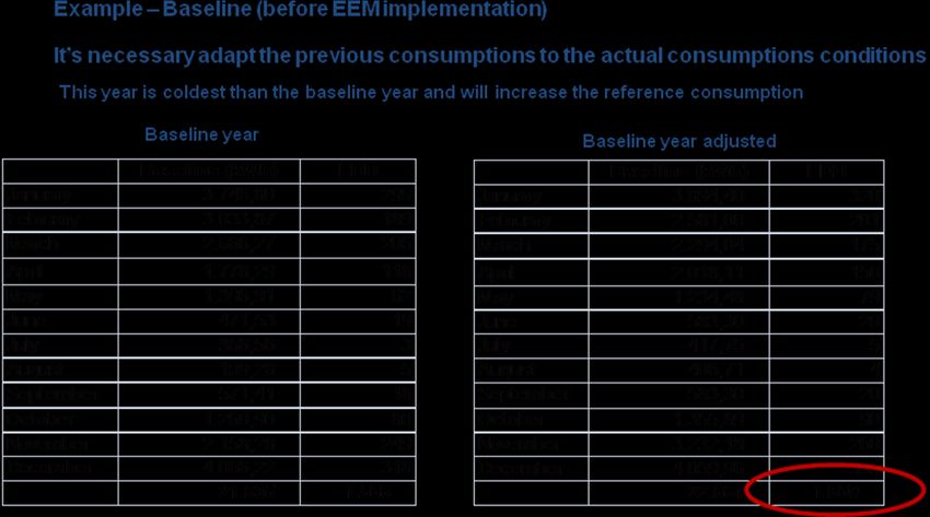
TABLE OF CONTENTS
1         Introduction .......................................................................................................................... 5

    1.1   Purpose of this document ........................................................................................................... 5

    1.2   Document structure .................................................................................................................... 5

    1.3   The measurement protocol IPMVP ............................................................................................. 5

    1.4   IPMVP measurement options ..................................................................................................... 7

2         The ICT PSP methodology for the measurement of energy savings and emission reduction 10

    2.1   Introduction .............................................................................................................................. 10
          2.1.1       Savings measurements are based on estimation of non-intervention consumption                                                  10

          2.1.2       Assessment of IPMVP options in the context of ICT PSP                                                                         10

    2.2   Foundations of the ICT PSP approach ....................................................................................... 12
          2.2.1       Independent and dependent variables                                                                                           12

          2.2.2       Intervention (treatment)                                                                                                      14

          2.2.3       Dependent variables and their units (ratios)                                                                                  15

    2.3   The ICT PSP approach – energy saving ...................................................................................... 17
          2.3.1       Pre-post comparison                                                                                                           17

          2.3.2       Outside temperature as independent variable                                                                                   19

          2.3.3       Selection of reporting period                                                                                                 22

          2.3.4       Summary of steps for estimation from baseline                                                                                 23

          2.3.5       Applying control group techniques                                                                                             23

          2.3.6       Control group approach to behavioural changes                                                                                 25

          2.3.7       Measurement of independent variables by user survey                                                                           26

    2.4   The ICT PSP approach – peak demand reduction ..................................................................... 27
          2.4.1       Interventions to reduce peak demand                                                                                           27

          2.4.2       Use of the load factor metric                                                                                                 29

          2.4.3       Estimator as average over 10 day baseline                                                                                     30

          2.4.4       Estimator as average of top 3 of 10 day baseline                                                                              30

          2.4.5       Estimator as average of top 3 of 10 day baseline with morning adjustment                                                      31

          2.4.6       Estimating CO2 emissions                                                                                                      32

3         Example applications .......................................................................................................... 33

    3.1   Use of working tables in eSESH ................................................................................................. 33

    3.2   Applying IPMVP Option C in 3e-Houses .................................................................................... 34

    3.3   Evaluation of user behaviour in eSESH - longitudinal three-stage-design ................................ 36

    3.4   Evaluation of social and behavioural changes in 3e-Houses – a longitudinal two-stage design47

                                                                                                                                                           3
4         Further information ............................................................................................................ 56

    4.1   Comparison between pilot results in different EU member states........................................... 56

    4.2   Understanding user behaviour.................................................................................................. 56

    4.3   Other information sources ........................................................................................................ 62

5         List of figures and tables ..................................................................................................... 63

                                                                                                                                                  4
1         Introduction

1.1        Purpose of this document
In response to the Third Call for Proposals under the ICT PSP Work Programme 2009, Objective 4.1 –
“ICT for energy efficiency in social housing”, three projects have been selected:
      -     3e-HOUSES: Energy Efficient e-HOUSES
      -     E3SOHO: Energy Efficiency in European Social Housing
      -     eSESH: Saving Energy in Social Housing with ICT

The three consortia were asked to work on the development of a methodology for energy saving
measurement – the current status is presented in this document. The 1st version of this document
has been completed by 3e-HOUSES1 in September 2010.

This document contains the updated version of this document and uses all information provided in
the first version. In this version it has been tried to concentrate on information directly related to
energy saving measurement which means that information provided in the previous version
regarding 3e-HOUSES pilots has been partly removed. Information about all three projects is publicly
available on the project websites.2

1.2        Document structure
The document is structured as follows:

Chapter 1.3 includes a brief summary of the IPMVP protocol and its options as the basis for the
methodology described in chapter 2.
Chapter 2 contains “The ICT PSP methodology for the measurement of energy savings and emission
reduction”. It asses the different IPMVP options and outlines the foundations of the ICT PSP
approach for energy saving and peak demand reduction.

Chapter 3 contains project specific examples from eSESH as well as from 3e-Houses and chapter 4
lists sources for further information.

1.3        The measurement protocol IPMVP
The original basis for savings calculations within the ICT-PSP projects was a modified version of the
EVO International Performance Measurement & Verification Protocol (IPMVP).

The IPMVP was originally developed by the U.S. Department of Energy, was first published in 1996
under the name NEMVP and is now owned by an international not-for-profit organisation EVO.
According to the EVO site (www.evo-world.org) the protocol is the leading international standard in
measurement and verification protocols. The IPMVP is defined in three volumes3:

1
  http://www.3ehouses.eu/sites/default/files/3e-HOUSES_Deliv_1-2_Definition_of_Methodologies.pdf
2
  www.eSESH.eu - www.3ehouses.eu - www.e3soho.eu
3
  All documents are available after a short registration at www.evo-world.org
                                                                                                    5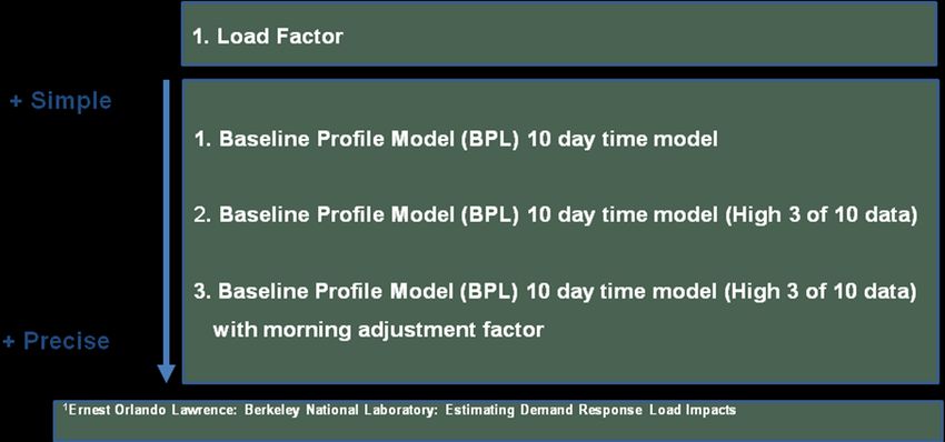
Concepts and Options for Determining Energy and Water Savings, Volume 1, (September
2010)
Concepts and Practices for Improved Indoor Environmental Quality, Volume 2, (March 2002)
Concepts and Practices for Determining Energy Savings in New Construction, Volume 3/I
(January 2006)
Concepts and Practices for Determining Energy Savings in Renewable Energy Technologies
Applications, Volume 3/II, (August 2003)
The IPMVP was designed to reduce risk for investors in energy performance contracting by providing
an agreed method for estimating energy savings to be shared between contractual partners. The
protocol is designed explicitly for so-called “big energy efficiency projects” in the industrial sector, i.e.
those with annual consumption levels of over 1,000,000 kWh.
The current methodological proposal for ICT PSP projects in the residential sector sets out from the
IPMVP and adapts its provisions to the very much smaller scale of energy consumption in the
residential sector and to the different purpose of providing feedback on the success of attempts to
save energy in that sector.
One early adaptation of IPMVP to ICT PSP was to attempt to reduce costs of measurement in line
with the dramatically lower scale of energy consumption by suggesting the use of larger time
intervals for measurement and the use of less sub- metering. It was found that the IPMVP approach
is in parts applicable to the residential sector, in particular, notions of baseline and methods of
calculating savings.
However, there are parameters such as demand response and avoided CO2 emissions which are not
taken into account in the IPMVP protocol and where extensions are required4. To calculate the CO2
emission savings from energy use savings, the overall consumption of electricity and of particular
fuels for heating can be converted to CO2 using standard combustion coefficients for fuels and a
coefficient for CO2 emission per kWh electricity generated based on the national mix of generation
sources. The calculation of CO2 emission savings is of course quite different in the case of successful
“peak-shaving” (see chapter 2.4).
The IPMVP measurement and verification plan (M&V Plan) includes the following 13 topics (IPMVP,
vol. 1, page 39 ff.):
1. Intent of energy conservation measures (ECM): Description of the planned services,
conditions and intended results
2. Selection of option and measurement boundary: IPMVP differentiates between four options
to specify determinations of savings (IPMVP, vol. 1, p21f and fig. 3, p37)
3. Definition of baseline: Period, energy data and conditions (independent variables such as
outdoor temperature; static factors such as building characteristics or equipment inventory)
4. Definition of reporting Period: Period after intervention, e.g. installation of EAS or EMS
4
Ernest Orlando Lawrence: Berkeley National Laboratory: Estimating Demand Response Load Impacts
6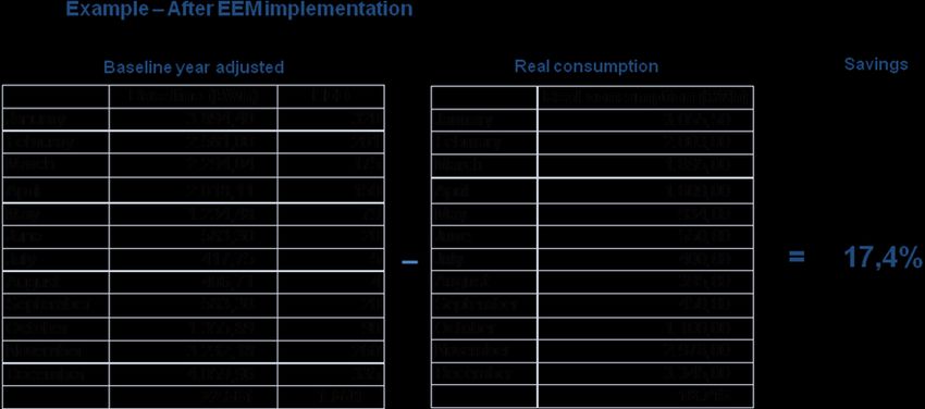
5.      Definition of basis for adjustment: Description of a set of conditions to which all energy
                measurements will be adjusted (e.g. temperature adjustments)
        6.      Specification of analysis procedure: Used statistical data analysis procedures
        7.      Specification of energy prices: Prices that will be used to value the savings (of importance in
                cases of adjustment needs because of prices changes)
        8.      Meter specifications: Description of metering points and periods (of importance in cases of
                not continuous energy consumption metering)
        9.      Assignment of monitoring responsibilities: Definition of responsibilities for recording and
                reporting of energy data
        10.     Evaluation of expected accuracy: Statistical accuracy of the measurement
        11.     Definition of budget required for savings determination: Initial set-up costs and ongoing
                costs throughout the reporting period
        12.     Specification of report format: Description of how result will be reported and documented
        13.     Specification of quality assurance: Description of quality assurance procedures

In summary an M&V Plan mainly focuses on meter installation, calibration and maintenance; data
gathering and screening; development of computation methods and – if necessary – acceptable
estimates; computation of measured data and reporting, quality assurance and third-party-
verification of reports.

1.4   IPMVP measurement options
In IPMVP, four options A-D are given for measurement and verification.

OPTION A. Partially Measured Retrofit Isolation:

Savings are determined by field measurement of the key performance parameter(s) which define
the energy use of the implemented Energy Efficiency Measures (EEMs) in the affected system(s)
and/or the success of the project.
The parameters which are not selected for field measurement are estimated. These estimates can
be based on historical data, manufacturer’s specification, or engineering judgment. A
documentation of the source or justification of the estimated parameters is required. The plausible
savings error arising from estimation rather than measurement is evaluated.

Measurement frequency ranges from short-term to continuous, depending on the expected
variations in the measured parameter, and the length of the reporting period.

Using Option A only partial measurements will be carried out in the parts which are affected by the
implementation of the energy efficiency solution with some parameters stipulated rather than
measured. The stipulations can be done only, if it is sure that there is no impact on overall reported
savings from these parameters.

To isolate the energy use of the EEM-system affected equipment from the rest of the facility,
measurement equipment shall be used. This equipment works as a boundary between affected and
non-affected equipment.
As said, stipulations are partly allowed under Option A, but great care has to be taken to review the
engineering design and installation to ensure that all stipulations are realistic and achievable. With

                                                                                                             7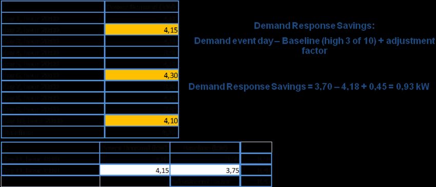
the use of stipulations of different parameters certain insecurity is created. Only very realistic
estimations should be done (e.g. a reduction of operating hours of the lighting with using of the
same equipment) in order to calculate the savings.
This option could be chosen to calculate energy savings if there are changes of lamps, appliances,
thermal equipment or changes of operating times.
Example of application: A lighting retrofit where power draw is the key performance parameter
that is measured periodically. Estimate operating hours of the lights based on building schedules
and occupant behaviour.
How Savings are calculated:
Savings = Base year – Post-Retrofit ± Adjustments
It is necessary to calculate the baseline and reporting period energy consumption from:
short-term or continuous measurements of key operating parameter(s)
estimated values
Sub-metering ECM affected systems.
Routine and non-routine adjustments are required.
OPTION B. Retrofit Isolation: All Parameter Measurement
The savings determination techniques of Option B are identical of those of Option A except that no
stipulations of parameters are allowed under Option B. This means that full measurement is
required, which makes this option a more expensive solution for measurements in energy
consumption and determination of energy savings. On the other hand more accurate and reliability
of results are obtained with this option.
Savings are determined by field measurement of the energy use of the EEM-affected system.
The measurement frequency ranges vary from short-term to continuous, depending on the
expected variations in the savings and the length of the reporting period.
There are short-term or continuous measurements in baseline and reporting period energy. Routine
and non-routine adjustments are required.
The savings created by most types of EEMs can be determined with Option B, but it is to consider
that the costs associated with the verification increase as well as metering complexity increases too.
Examples of application: Application of a variable speed drive and controls to a motor to adjust
pump flow; measure electric power with a kW meter installed on the electrical supply to the motor
which reads the power every minute. In the baseline period this meter is in place for a week to verify
constant loading. The meter is in place throughout the reporting period to track variations in power
use.
OPTION C. Whole Facility
Option C involves the use of utility meters, whole building meters or sub meters to assess the
energy performance of a total building. All the EEM systems savings are to be assessed with this
option, so it will include all consumptions and savings of different EEMs, so preferably this option is
8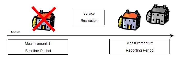
suitable for one type of EEM. If different EEMs are applied the collective savings will be estimated
from the energy meter of the whole facility and therefore cannot be distinguished.

Savings are determined by measuring energy use at the whole facility or sub-facility level.
Continuous measurements of the entire facility’s energy use are taken throughout the reporting
period.

The whole facility baseline and reporting period (utility) meter data will be analysed. Routine
adjustments are required, using techniques such as simple comparison or regression analysis. Non-
routine adjustments are required.

Examples of application: Multifaceted energy management program affecting many systems in a
facility. The energy use with the gas and electric utility meters for a twelve month baseline period
and throughout the reporting period will be measured.

Option C should be used if there are many types of EEMs in one building/housing and if the energy
performance of the whole building/housing is to be assessed.

This option is indicated for energy efficiency measurements application with total energy savings
potential higher 10%.

OPTION D. Calibrated Simulation

Savings are determined through simulation of the energy use of the whole facility, or of a sub-
facility. Simulation routines are demonstrated to adequately model actual energy performance
measured in the facility. This Option usually requires considerable skill in calibrated simulation.

Energy use simulation, calibrated with hourly or monthly utility billing data. (Energy end use
metering may be used to help refine input data.)

Examples of application: Multifunctional energy management program affecting many systems in a
facility but where no meter existed in the baseline period. Energy use measurements, after
installation of gas and electric meters, are used to calibrate a simulation. Baseline energy use,
determined using the calibrated simulation, is compared to a simulation of reporting period energy
use.

                                                                                                   9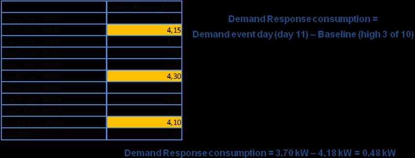
2     The ICT PSP methodology for the measurement of energy savings and
      emission reduction

2.1     Introduction

2.1.1    Savings measurements are based on estimation of non-intervention consumption

Energy savings due to an Energy Saving Intervention (ESI) cannot be measured directly, as they
represent the difference between energy actually consumed after the intervention and that which
would have been consumed had the intervention not been carried out. For policy in an ICT PSP
context it is also important to anticipate the impact should the intervention be applied more widely,
that is for example, what the overall energy saving would be if the ICT applications developed and
applied in the pilot were applied to all residential buildings in Europe.

Because energy saving cannot be measured directly, any measurement is in fact based on
assumptions of a possible parallel development – the development of energy use without the
intervention: “non-intervention consumption”.

2.1.2    Assessment of IPMVP options in the context of ICT PSP

Constant demand – IPMVP Options A and B

The simplest assumption of how demand in a building would develop without the intervention is that
demand for energy in a building is constant. If demand is constant, the intervention would reap
savings perhaps by making the conversion of primary energy into the heat / coolness / cooked meal /
well-lit rooms more efficient.

The energy saving measurement methodology for this case is simplicity itself. Energy savings can
simply be measured by the change in energy consumption before and after the intervention. Given
24/7 constant demand with no stochastic variability, only one measurement would be needed. More
measurements and some averaging might be needed if the measurement apparatus exhibits error -
or because the energy conversion efficiency of the ICT application varies over time (warm-up phase
for lamps etc.).

In the industrial settings addressed by IPMVP there may be examples of constant demand, e.g. a
pump operates continuously at the same load while production plant is in operation; the hallway
lighting is on 24/7 etc.

In cases of constant demand it may not even be necessary to make any measurement in situ. IPMVP
Option A captures this allowing that the manufacturer’s specified efficiency improvement in a light is
used for the savings calculation and that this is acceptable to the ESCO contracting partners.
Even in IPMVP, however, situations of varying demand have a central role. Production processes may
not run at the same capacity all the time, may be shut down etc. A pumping operation may take
place at regular intervals, not continuously. Measurement of savings from an intervention which
involves installing a more efficient pump may need only one measurement, but this needs to take

                                                                                                   10
place at a point where demand is known to be equal to the comparison value from before the
intervention – the “constant loading” mentioned in Option B.
This mode of thought led to the development of the options A and B in IPMVP. A corollary to Options
A and B is that any energy saving intervention planned or executed would be in no need of an ICT PSP
pilot to prove the saving level in a statistically representative sample.
Options A and B therefore seem to be uninteresting in the context of ICT PSP.
Modelling variable demand – Option D
IPMVP also deals with less simple cases, where demand varies in a less predictable way, where there
is no repeated pumping cycle in which a point of equal demand can be identified. For example, even
when production is running at the same capacity, flows of raw materials or heating processes may
vary in demand due to variation in input temperatures of the raw materials, their specific weight,
consistency etc. This demand variability is a major cause of the complexity of methodology proposed
under IPMVP.
In a machine production environment, the factors causing variability of demand are often accessible
and even measurable. Where the processes under consideration are well understood, one solution is
to model the variability. However, if an accurate model can be set up, this must contain parameters
encapsulating the energy saving, and once set up, no additional measurements would be needed,
certainly not over a 12 month operation period.
Again, Option D seems to be uninteresting in the context of ICT PSP pilot.
Variable demand as a result of the ICT application – Option C
In the residential sector, an assumption of constant demand (Option A) or cyclically predictable
demand (Option B) or another demand structure which can be fully modelled (Option D) cannot
usually be made. In particular, none of these assumptions applies to projects aiming to change the
resident behaviour – i.e. change demand – as a key way in which the intervention takes effect, such
as many interventions being piloted in the ICT PSP projects.5
In the ESCO contracting situation, the ESCO will not implement interventions which change demand;
responsibility for changing levels of demand will be contractually assigned to the user organisation
and the commercial impact as well. If energy consumption rises not because of poor performance by
the solution provider but because of increased demand, the ESCO will typically want this corrected –
adjustments have to be made to correct the demand and the energy saving to what it would have
been under constant (or contractually agreed) demand. Thus IPMVP, supplying solutions into this
contractual relationship, bases all options on the usual separation of demand (user organisation
responsibility) and supply (ESCO responsibility).
Nevertheless, the approach offered in IPMVP as Option C is certainly applicable in an ICT PSP context.
This option does not assume constant energy demand or that energy demand variation can be
accurately modelled. Option C is a before-after comparison. The IPMVP approach in Option C still
5
e.g. the piloted Energy Awareness Services for tenants in eSESH or the Resource use Awareness Services for tenants in
BECA
11carries the notion of fully repeated cyclical variation in demand. This is exposed in the notion of an
“operating cycle”, (IPMVP, Vol. 1, p15), however, with some adjustments the approach is still
applicable to ICT PSP pilots. The ICT PSP methodology presented here also allows for a control group
approach, not defined in IPMVP (and likely to be inappropriate in ESCO contracting).
2.2 Foundations of the ICT PSP approach
2.2.1 Independent and dependent variables
Before introducing the ICT PSP methodology, it is important to introduce an understanding of key
terms such as dependent and (relevant) independent variables, and, for the before-after approach,
the idea of baseline and reporting period.
Independent and dependent variables are understood as follows:
Independent Variable: Characteristics of a building, its environment or use which affect
energy consumption: weather (temperature, humidity), occupancy, dwelling size, heating
system, etc. When reference is made to an independent variable, the implication is that it
has an impact on demand. Some such variables can be easily measured – e.g. ambient
temperature – others may be more difficult to measure.
Dependent Variable: Characteristics of a building or its use which is the target of an
intervention. Here the main focus is (reduction in) energy consumption, which can be related
to the scale of the intervention as number of tenants (kWh per person) or the size of the
dwellings (kWh per square meter).
In before-after comparison, the actual energy saving caused by an Energy Saving Intervention (ESI) is
estimated from the difference between consumption after the intervention (ESI) and the
consumption which would have taken place under the same demand conditions without the ESI.
To estimate what consumption would have been without the ESI, consumption data prior the
intervention is used. This is known as baseline data. An extended baseline is the projection of
consumption before the intervention into the period after the intervention.
Figure 2-1 shows the progress of energy consumption. To the left of the arrow the energy
consumption without the ESI is shown. With this data it is possible to create the baseline. To the right
of the arrow the consumption after the ESI is shown.
12Time (months)
Figure 2-1 – Progress of energy consumption
Until the shown point (arrow) in Figure 2-2 the consumption is needed to create the baseline. The
continuation of the baseline, the extended baseline, shows the expected consumption without the
ESI, however, if the ESI is implemented this continuation does not take place and cannot be
measured directly. The period after the intervention during which measurement of saving takes
place is referred to as the reporting period.
Time (months)
Figure 2-2 – Baseline before ESI implementation
The arrow in Figure 2- 3 divides both parts in the “baseline period” and the “reporting period”
13Time (months)
Figure 2-3 – Baseline before ESI and progress of energy consumption
After the ESI has been implemented (reporting period), the consumption is expected to be lower
than it would be had the baseline continued. For better understanding, the following Figure 2-4
shows the energy savings after the implementation:
Time (months)
Figure 2-4 – Energy savings
2.2.2 Intervention (treatment)
Another important concept is that of the intervention: the action from outside which has been
undertaken to reduce energy consumption in a particular domain. There are other terms used for
intervention. For example, when evaluating the behaviour-related effects of consumption feedback
services, the empirical social research terms that service as treatment. The term is originated from
psychological experiments which are used to establish cause and effect of measures, instruments,
etc. The main characteristic of experiments is the availability of two (tenant) groups – the
14experimental or treatment group which receives the treatment and the control group which receives
no treatment. Control group approaches are discussed below.
2.2.3 Dependent variables and their units (ratios)
To make figures on energy saving comparable despite different sizes of dwelling, times of year,
number of occupants etc., specific units can be used in presentation which set levels of energy
consumption or energy saving in relation to the size of the unit considered. Specific units can be
useful to show the dependency of energy savings on independent variables such as floor area,
occupancy or ambient temperature, or to remove the influence of these variables when comparing
two savings measures. Which units are appropriate depend to some extent on the type of energy use
in question.
Also, as pointed out above, there is not a direct relationship between the energy saved in the final
energy form (using kWh as primary unit) in the form of primary energy (using kWhPE as primary unit)
and CO2 emission savings (e.g. using tonnes of CO2 as primary unit). Which primary unit is being used
must be made clear. Some examples of appropriate specific units by function are:
Heating:
Energy consumption (saving) per dwelling (kWh/dwelling p.a.)
Energy consumption (saving) per person (kWh/person p.a.)
Energy consumption (saving) per square meter (kWh/m2 p.a.)
Energy consumption (saving) per degree-day KWh/HDD p.a. (Heating Degree Days)
Primary Energy consumption (saving) per square meter (kWhPE/m2 p.a.)
Share of renewable energy (%)
Cooling:
Energy consumption (saving) per dwelling (kWh/dwelling p.a.)
Energy consumption (saving) per person (kWh/person p.a.)
Energy consumption (saving) per square meter (kWh/m2 p.a.)
Energy consumption (saving) per degree-day KWh/CDD p.a. (Cooling Degree Days)
Primary Energy consumption (saving) per square meter (kWhPE/m2 p.a.)
Share of renewable energy (%)
Electricity:
Energy consumption (saving) per dwelling (kWh/dwelling p.a.)
Energy consumption (saving) per person (kWh/person p.a.)
Energy consumption (saving) per square meter (kWh/m2 p.a.)
Primary Energy consumption (saving) per square meter (kWhPE/m2 p.a.)
Share of renewable energy (%)
Domestic Hot Water (DHW):
Energy consumption (saving) per dwelling (kWh/dwelling p.a.)
Energy consumption (saving) per person (kWh/person p.a.)
15 Primary Energy consumption (saving) per person (kWhPE/person p.a.)
Share of renewable energy (%)
Cold water
Water consumption (saving) per person (litre /person p.a.)
Avoided CO2 emissions
CO2 avoided emissions (kgCO2/a) = energy savings (kWh/a) * emission factor (kgCO2/kWh)
The emission factor depends on the type of energy saved, for example:
Electricity: depending on the composition of the electricity generation mix of each country in
each moment.
Natural gas: 0,201 (kg CO2/kWh)
Diesel: 0,287 (kg CO2/kWh)
Before moving to an economic view, it is important to note that for residents in particular, energy
savings are not the only relevant output of an ESI. An important additional output variable for HVAC
functions is the subjective “comfort” experienced by residents, which is partly captured by
objectively measurable values such as room temperature and relative humidity in the dwelling. The
impact of humidity and a range of gaseous or fibrous particles like CO, Radon, Ozone, fibers, etc. on
Indoor Environmental Quality (IEQ) is addressed in IPMVP Volume 2. High relative humidity may
contribute the growth of fungi and bacteria dangerous to health. The additional relevant units here
are:
Room air temperature (degrees C)
Relative humidity (%)
From an economic perspective, energy savings may represent the return on an economic investment.
The return on this investment can be illustrated by setting savings in relation to size of investment in
different ways. Key variables here are the conversion of consumption figures in kWh and litres of cold
water into EURO, using market prices:
Cost of consumption (saving) per dwelling (€/dwelling)
Cost of consumption (saving) per person (€/person)
Cost of consumption (saving) per square metre (€/m2)
Particularly where the investor and/or recipient of energy bills is a private person, issues of
affordability – proportion of disposable income – may play a role, such that cost might be
expressed as a proportion of per capita (disposable) income:
Cost of consumption (saving) as proportion of per capita income (%)
Looking at the return on investment, key ways of expressing investment success are:
Net present value of the investment per square metre (€ / m2 )
Return on investment (ROI) (%).
16Finally, for reasons of assessing the likelihood of further exploitation of results it may be
important to report the level of public funding:
Public funding [%]: Share of public funding in the energy saving investment.
2.3 The ICT PSP approach – energy saving
2.3.1 Pre-post comparison
As outlined above, measuring energy savings requires estimation of consumption which would have
taken place had the intervention not been carried out, the “non-intervention consumption”.
Estimates of non-intervention consumption can be based on extrapolation of consumption in a
period before the intervention. The result of an energy saving intervention is estimated through
comparison of measured energy consumption data before (baseline period) and after the
intervention starts (reporting period).
Ideally a model has been built which shows how energy use varies under the influence of
independent variables, such as outside temperature, occupancy, household size etc.
If no independent variables can be measured, the selection of a baseline period is critical. This period
should be such that all known but unmeasured independent variables exhibit a full range of variation
during the baseline period.
Figure 2-5 – Before-after-analysis of one building
If for example demand varied month by month during the year but was the same for the same month
of each year, it would be important either to ensure the baseline covers a full year, or to ensure
baseline and reporting period cover the same months in different years. Of course this does not fully
reflect key residential patterns – holidays are not just taken in different months but also for different
periods, and for heating bills years are not the same on average nor are months directly comparable.
Measuring baseline data is a costly exercise, and the quality of the decisions can impact on the
accuracy and validity of conclusions on energy savings. Decisions on length and timing of baseline
measurement are therefore very important. Depending on the independent variables affecting the
consumption which is targeted, different decisions will be taken about the appropriate length of
baseline – day, week, month or year.
If it can be assumed that domestic hot water consumption is quite similar from day to day during the
whole year, baseline data from one day would be enough. If mild variation is expected, this might be
extended to a week. This of course raises the question as to why a 6 or even 12 month operation
17period would be needed for the reporting period data. Similar considerations might apply to cold
water consumption, however, it is even clearer here that garden-watering and swimming-pool use is
seasonal, and weather-dependent, so that longer periods of monitoring would be advisable – or the
building of a statistical model based on multiple independent variables.
The recommended approach is to develop regression models that reproduce the energy
consumption based on values of the independent variables.
Climatic changes are the main reason of variability in residential consumption profiles. Average
temperature or heating degree days (HDD) and cooling degree days (CDD) can be used.
Whereas in the industrial production plant targeted by IPMVP there may be repeated periods of
energy use making up something which can be referred to as an energy use cycle, this is not the case
in domestic energy consumption. Therefore, no suggestion for linking particular baseline periods to
particular energy uses – a week for hot water, a year for heating - is given in the methodology.
For regression models an adequate accuracy of modelling of the variation in the dependent variable
is necessary to accurately estimate the extended baseline – the no-intervention consumption - in the
reporting period.
One metric for goodness of fit is the squared multiple correlation coefficient R2, which reflects the
proportion of variance explained in the model. If R2 is low, further independent variables must be
found to improve predictions. If R2 remains low, only very large savings of energy will be reliably
detected.
The IPMVP suggestion to include only months with more than 50 degree days in the analysis6 is
appropriate only if the cost of data gathering can be reduced this way, and the energy savings in
warmer months is insignificant in the impact of the intervention as a whole.
Baseline (kWh) HDD
January 3.746,80 299
February 3.033,87 189
March 2.666,27 206
April 1.778,29 118
May 1.396,91 62
June 471,53 19
July 366,56 3
August 109,28 5
September 571,41 18
October 1.269,90 80
November 2.158,28 249
December 4.066,22 318
21.635 1.566
Figure 2-6 – Baseline consumption and baseline degree days
6
IPMVP, vol. 1, p. 83.
18Figure 2-7 – Table and graph of energy consumption related to HDD
Figure 2-7 shows a regression line reflecting a correlation between monthly consumption and HDD.
More than 90% of variance is explained, which suggests that accuracy of estimation is very good. In
fact, a model such as this, of energy consumption for heating of a building in regular use, built with
an independent variable reflecting ambient temperature such as degree days and using data for an
entire year, will normally have a high R2. The high value reflects the very high variability of the
dependent variable, heating consumption over the year, rather than showing the model is adequate
for detecting energy savings due to an intervention. This variability must be reduced to show the
impact of even the most effective intervention.
2.3.2 Outside temperature as independent variable
Within the EU a number of calculation models are in use to reflect outside temperature changes over
time. Examples are given from Germany, France and Belgium.
In Germany there are a number of different standards for heating degree days, based on different
heating limit temperatures (heating degree days and of degree-day numbers – HDD, outdoor
temperature 15°C or less)7:
HDDHeizgradtage/heating degree days = Heating limit temperature (10, 12, 15) – Daily average outside temperature
[This formula is used for a climate adjustment.]
HDD Gradtagszahl/degree-day numbers = Inside temperature (20) – Daily average outside temperature.
[This formula is used if solar and internal gains should be taken into account too.]
2
Specific energy consumption figures (kWh/m ) can be divided by DDHeizgradtage resp. DDGradtagszahl. The quotient is
2 2
a figure in kWh/( m *Kelvin-days) (or *24/1000 in m *Kilo Kelvin Hours).
In France the heating limit temperature (external temperature baseline) amounts 18°C. The degree
day correction is divergent as well and is calculated as follows:
7
Passive house standard 10°C, 50°F; low energy standard 12°C, 53,6°F; all the rest of buildings (building stock)15°C, 59°F. The use of equal
heating limit temperatures in order to determine the number of degree days in both baseline and reporting period is obligatory.
19[Calculation of heating degree days: Average between maximum and minimum outside temperature]
The calculation of the degree days in Belgium is the same as the calculation of DDheating degree day in
Germany. In Belgian the tradition is to use a heating limit temperature of 16, 5°C.
For purposes where the consumption over a short period is to be corrected or compared, Belgian
practice is to take account of the delay effect / thermal inertia of buildings by using ‘equivalent
degree days’ to take account of energy saved in building structure from previous days, as follows:
DDequiv = 0.6 x DD (today) + 0.3 x DD (yesterday) + 0.1 x DD (day before yesterday).
For purposes such as the issuing of energy performance certificates of buildings it is customary in
Germany to use long-term averages from weather data over a period of 30 to 40 years. Given this or
another appropriate standard for outside temperature, e.g. the average number of heating degree
days over a long period, measured data – baseline or reporting period - can be converted to energy
consumption in a “standard” year.
Figure 2-8 – Degree day correction with temperatures of a standard period
This method can be used not only to correct baseline data to a standard year, but also to correct the
reporting period data to a standard year. When the temperature adjusted consumption data of the
reporting period is subtracted from the consumption data of the baseline period this represents the
saving which would have been achieved in a standard year.
One minor point to be taken into account here is that if reporting period figures are also adjusted to
a standard year, then for transparency the saving figure calculated must be reported as “energy
saved in a standard year”, and not presented as the amount of energy saved in the specific ICT PSP
pilot. And yet more minor is the point that given long-term global temperature trends, the value of
standard years may be seen as diminishing, to be replaced by a projection of expected temperature
over the investment pay-off period.
A much more important issue is the effectiveness of this approach for the purpose of evaluating ICT
PSP pilots.
Given the powerful influence of outside temperature on energy consumption for heating, it is
effectively being assumed that the only independent variable to be considered is outside
20temperature, and that this simple correction to differences in average outside temperature can be
performed to show the energy saving. The effect of the independent variable is removed.
If this were indeed the only independent variable, the level of consumption, measured in
kWh/Kelvin-days, would be constant during the baseline, and during the reporting period. The value
of R2 would be 1.0, showing that all variance had been explained. Given this constancy, the
measurement period for baseline and reporting period could be shortened to any single day,
radically reducing the costs of piloting in ICT PSP. This assumption is of course far from reality.
Multiple factors affect the level of energy consumption for heating apart from outside temperature.
A simple example is the setting of thermostatic valves in radiator systems. If this setting is changed,
the linear relationship between outside temperature and kW of energy lost through building walls
shifts up or down in response. The setting of the valve is an independent variable – it does affect
energy consumption.
This behaviour-related effect is important in the choice of baseline and reporting period, not the
physical effect of ambient temperature on conduction processes through building walls.
If the valve is used by the resident to shut down the heating during a winter holiday, and the baseline
period falls during this holiday, it will be difficult to show any energy saving from a subsequent
intervention. The opposite is true where the reporting period falls in the holiday period. Here a
simple degree day correction is inappropriate.
Looking at different energy uses makes this point more forcibly. To detect a change in the use of
energy for the purposes of running household electric appliances, caused by a specific energy saving
intervention, simply applying a “degree day correction” to baseline and reporting period would be
obviously unacceptable.
Such considerations, and not the influence of climatic variables on which accurate data is available,
are the reason both for extending measurement periods and using statistical techniques such as
regression.
In the case of energy use for heating, degree days could be used in an initial conversion of raw
energy data to a new statistic in kWh/Kelvin-day which is then taken ahead in statistical analysis to
detect the reduction in energy use due to the energy saving intervention. However, as the following
considerations show, it may not be appropriate to use degree days in this way, or even as
independent variable in regression analysis.
There are multiple metrics for outside temperature variation. Degree days may be calculated using
10, 12, 15, 16.5 or 18 degrees Centigrade as cut-off (compare above). Data on average daily
temperatures is available from networks of meteorological stations, and dedicated measurement
could be used from the buildings in the pilot to provide hourly or even more frequent temperature
values.
For the purposes of estimating real energy savings in ICT PSP pilots, the choice of an outside
temperature metric is not guided by normative considerations such as is the case in certification.
Instead, the metric should be as accurate a reflection as possible of the linear influence of changes in
outside temperature on the loss of heat from a heated building, so that the real behaviour of heating
21systems controlled by residents can be modelled. Where residents are able and do set their heating
system to provide inside temperature of over 20 degrees, most degree day statistics lose predictive
power. The error is likely to be minor, however. The small value at the regression line intercept in
Figure 2-9 probably reflects an error due to this discrepancy.
Unlike the German and Belgian degree days, with their normative assumptions of appropriate levels
of temperature inside heated buildings, the “energy signature” customary in France is based on
outdoor temperature without coding into degree days.
Figure 2-9 represent the energy signature of a building, showing the use of outdoor temperature in
the regression equation. In the region to the right where the outside temperature is above the 18
degrees room temperature applied to social housing in France, the residual energy consumption
represents the consumption of domestic hot water.
The energy signature, i.e. the complete plot of consumption against temperature, is predominantly
used in France to analyse energy requirements and operating costs of a building. Its relevance here is
to show that direct use of outside temperature metrics in statistical analysis without conversion into
degree days is feasible.
Figure 2-9 – Example of an Energy signature
2.3.3 Selection of reporting period
After the ESI and a following period with improvements/adjustments, the energy savings should
remain stabilised for a certain period of time in the case where tenants are involved. To monitor the
persistence (increase or decrease) of energy savings in the time it is necessary to roll out the
following steps:
In the short term, it is possible to compare each week to analyse if the energy savings are
continuous over time after the energy saving intervention, especially if the savings depend
on social behaviour.
For equipment renovations it is very important to verify in the long-term too.
222.3.4 Summary of steps for estimation from baseline
In the before-after comparison approach, six steps are necessary:
1. Nominate a time period for the baseline which captures all variation of immeasurable
independent variables and can yield an average which can reasonably be expected to be
repeated in the future;
2. Gather data for the energy consumption (dependent variable) and for all accessible
independent variables (baseline period);
3. Perform a regression analysis to establish the coefficients for each independent variable;
4. Nominate a time period for the reporting period which is again long enough to capture all
variation of immeasurable independent variables8;
5. Gather data for the energy consumption (dependent variable) and for all accessible
independent variables (reporting period);
6. Apply the coefficients estimated in the baseline to the reporting period, yielding the result:
energy saving as the difference between estimated and measured consumption.
2.3.5 Applying control group techniques
As stated above, energy savings due to an ESI cannot be measured directly, as they represent the
difference between energy actually consumed after the intervention and that which would have
been consumed had the intervention not been carried out. Any measurement is in fact based on
assumptions of a possible parallel development – the development of energy use without the
intervention: “non-intervention consumption”.
There is no alternative but to estimate non-intervention consumption. Without this estimation there
is no energy saving “measure”. Estimation can be based on prior consumption patterns or on
patterns of consumption in comparable settings unaffected by the intervention – “control buildings”
– or on both.
Up until now we have dealt with using prior consumption for estimation, using baseline energy
consumption to estimate regression coefficients in order to re-applying these in the reporting period
to gain an estimate.
An additional or alternative source of estimation is a control group or control building approach.
Where no baseline energy consumption data are available – for example in case of new construction,
the control group approach would be the only alternative.9
8
E.g. the ICT PSP Work Programme refers to a 12 months period
9
Beyond the control group approach there are several different possibilities in order to get a baseline. But the control
group design is the recommended best option. For further information see IPMVP, vol. 3/1.
23Figure 2-10 – Control building design
A control building is a building which matches the characteristics of the experimental building in all
important respects, i.e. along all known independent variables. These can include for the building
itself:
kind of building,
location,
energy equipment,
insulation,
heating system
and for the building’s residents:
family structure,
proportion of families with young children,
proportion of employed and unemployed,
absence / holiday behaviour patterns,
use of building for occupational work,
etc.
If there are differences between the experimental buildings and control buildings or their residents,
these differences reduce the effectiveness of the control building approach. Differences open any
results to challenge using rival hypotheses for non-intervention consumption estimates,
hypothesised impacts of the differences. Despite the use of the word “hypothesis” here, the
undermining of results is real: the “hypotheses” stand alongside “estimates”, and have therefore
close to equally strong claims to be heard.
In the best of cases the only difference between experimental and control building is the presence or
absence of the ESI, for example tenants in the experimental building all have access to and regularly
use consumption feedback via a web portal whereas the tenants of the control building have no
access at all.
Practical considerations will usually prevent application of safeguards common in other domains,
where subjects are blinded to their inclusion in one group or another – it is not to be ignored that the
tenants of a control building, if they gained knowledge of the project and its purpose and their role in
the experiment, might change their energy-related behaviour, invalidating the “no-intervention”
24status – or where individuals are randomly assigned to experimental and control group – it is not to
be ignored that a pilot manager, wishing to show clear energy savings, might choose the most
advantageous buildings to be in the experimental group.
The advantage of a control building design is that data is collected over the same period in time,
therefore both control and experimental group experience other influences on their behaviour such
as a tightening credit crunch or a lengthening of school holidays. In the before-after approach, such
“history” influences would invalidate the comparison if they took place once some time after the
start of baseline and before data collection in the reporting period finished.
Using control buildings, there is the additional option of pairing buildings between experimental and
control group. In this case each pair must exhibit all the above similarities.
Implementing an evaluation using control buildings involves the following steps:
1. Select a group of buildings representative of the future exploitation potential of the energy
saving intervention (ICT application)
2. Divide the pilot buildings into 2 groups: treatment /experimental and control.
3. (Optionally) establish pairs of analogues cases from both groups.
4. (Optionally) measure dependent and independent variables during the baseline period in
each group
5. Implement the ESI in the treatment group
6. Measure dependent and independent variables during the reporting period
7. Use appropriate statistical techniques to estimate non-intervention consumption in the
treatment group during the reporting period based on baseline model and control group
model. Or use matched-pair statistical techniques to estimate the energy saving.
8. Calculate energy saving as difference between the estimated non-intervention consumption
and the measured energy consumption in the treatment group in the reporting period. Or
use matched-pair statistical techniques to estimate the energy saving.
2.3.6 Control group approach to behavioural changes
Where the intervention or treatment is the provision of an information service, a control group
approach can be applied. In the best of cases tenants can be assigned to control or experimental
group on a random basis. That means that all pilot tenants have the same probability to be part of
the control or the experimental group. In doing so, to both tenant groups nearly apply the same
conditions beside the relevant object of investigation (e.g. tenant portal). Ideally the control group
match the characteristics of the experimental group concerning living situation, household size,
average age, ecological awareness or the like. If there are behavioural or attitudinal changes in the
experimental group obvious, but not in the control group, then those changes can be interpreted as a
result of the treatment.
In some cases a control group approach is not appropriate because of the absence of comparable
buildings, too small sample sizes or a combination of both. In such cases other comparisons between
user groups can be considered. In the given context we can roughly differentiate three tenant
groups:
25 Experimental or treatment group with
o active users with full access and a regular use of services,
o passive users with possible access to services but without willingness to use,
Control-group without access to services.
When comparing active users and passive users only, systematic bias has to be taken into account.
Behavioural or attitudinal changes in the group of active users but not in the group of passive users
must be interpreted with caution. The passive users are not a randomly assigned control group. It has
to be taken into account that passive users seem to be not interested in the services at all or are not
able to use the service. That can be caused by several reasons which should be captured in the data
gathering and properly analysed.
Where a true control group cannot be built, it is expected to be helpful to differentiate not just
passive and active users but different levels of service use. For example, it may be helpful to
differentiate those who only use the service once or twice at the beginning from those who regularly
use the service. Which subdivision of type of service use is appropriate depends on the content of
the service, in particular the added information which can be gained by regular use compared to one-
off use.
2.3.7 Measurement of independent variables by user survey
The primary dependent variable, consumption of energy, is ideally measured by devices such as
smart meters, which once installed capture data continually and accurately. This is state-of-the art
for electricity, and increasingly for gas.
Some independent variables such as outside temperature can also be measured automatically and
reliably. This allows their inclusion in non-intervention consumption estimation without difficulty.
Others, such as the presence of children among residents, or periods of absence for work or holiday,
require the use of different techniques to “measure”, and as personal data are subject to data
protection legislation.
Energy-related behaviour and attitudes represent a large set of such independent variables. Several
ICT PSP projects have the common objective to develop ICT-based services to enable social housing
tenants to optimise their energy consumption behaviour. Key topics of the services are approaches
which deliver consumption feedback to the tenants for periods for less than a year which offer
possibilities of an energy monitoring and energy management and/or contain interactive
components like self-assessment-tools, benchmarking or alert systems. Differences can be found in
the specific design of the services, the sample sizes of pilot users, etc.
Where interventions target user behaviour, and user variables are to be included as independent
variables in the overall method, survey techniques can be used. When using surveys to measure
behaviour and other person-related factors or other factors relevant to energy consumption, it is
important to decide whether to use a cross-sectional study with one measuring point only or a
longitudinal study with multiple stages.
26You can also read