Directed Search and Competitive Search: A Guided Tour - School of Economics ...
←
→
Page content transcription
If your browser does not render page correctly, please read the page content below
Directed Search and Competitive
            Search: A Guided Tour∗
                      Randall Wright
  UW-Madison, FRB Minneapolis, FRB Chicago and FRB Atlanta
                          Philipp Kircher
       European University Institute & University of Edinburgh
                              Benoît Julien
                       UNSW Business School, Australia
                             Veronica Guerrieri
              University of Chicago Booth School of Business
                                    April 17, 2019

                                         Abstract
      This essay surveys the literature on directed search and competitive search
      equilibrium, covering theory and a variety of applications. These models
      share features with traditional search theory, but also differ in important
      ways. They share features with general equilibrium theory, but with explicit
      frictions. Equilibria are often efficient, mainly because markets price goods
      plus the time required to get them. The approach is tractable and arguably
      realistic. Results are presented for finite and continuum economies. Private
      information and sorting with heterogeneity are analyzed. While emphasizing
      issues and applications, we also provide several hard-to-find technical results.

  ∗
    For input we thank Timothy Cason, Michael Choi, Miguel Faig, Jason Faberman, Athana-
sios Geromichalos, Stella Huangfu, John Kennes, Ian King, Sephorah Mangin, Guido Menzio,
Espen Moen, Peter Norman, Andy Postlewaithe, Guillaume Rocheteau, Roberto Serrano, Shouy-
ong Shi, Robert Shimer, Scott Spitze, Ronald Wolthoff, Sylvia Xiao, Yiyuan Xie and Yu Zhu.
Wright acknowledges support from the Ray Zemon Chair in Liquid Assets at the Wisconsin School
of Business. Wright and Julien acknowledge support from Australian Reseaerch Council grant
DP170104229. The usual disclaimers apply.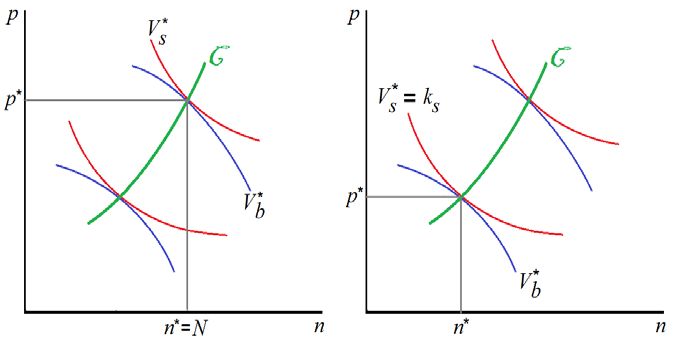
1         Introduction
Search theory contributes significantly to fundamental and applied research, and
is relevant for understanding many phenomena that are troublesome for classical
economics. Examples include the coexistence of unemployment and vacancies; price
or wage dispersion and stickiness; bid-ask spreads; the difficulties of bilateral trade
that generate a role for money and intermediation; partnership formation; long
and variable durations in the time to execute trades in labor, housing and other
markets; etc. This essay surveys a branch of the area concentrating on directed
search and competitive search equilibrium. While the plan in what follows is to
go into considerable detail on the literature, to give a hint up front, we mention
influential papers by Peters (1984,1991), Montgomery (1991), Shimer (1996) and
Moen (1997).1
        To be precise, for our purposes, an economic model has two components: an
environment, including descriptions of the set of agents with preferences and tech-
nologies; and a mechanism or solution concept mapping environments into outcomes.
Directed search is a feature of the environment. To explain this, first note that in
search theory agents are modeled as trading with each other, and often bilaterally,
different from Walrasian theory, where they simply trade with (slide along) their
budget lines.2 Directed search means agents see some, although perhaps not all,
characteristics of other agents, and based on that choose where to look for coun-
terparties. This contrasts with random search, where meetings are exogenous. The
characteristics of agents in most of the models described below include their posted
terms of trade — generally, contracts, although sometimes these are simply prices.
This contrasts with traditional search models that assume agents bargain after they
meet, and also with those that assume price posting when the posted terms do not
influence who meets whom.
        While directed and random search are different approaches that can be applied
in single-agent decision theory, competitive search equilibrium is solution concept
    1
     Highlighting a few papers like this was suggested by a referee, but it is not easy to know where
to draw the line. Other early related work includes Sattinger (1990) and Hosios (1990); one might
also say the papers reviewed in Section 5 were early and foundational; etc.
   2
     Some search models do have Walrasian pricing, e.g., Lucas and Prescott (1974) and Rocheteau
and Wright (2005) in labor and goods markets, respectively, motivated by saying agents meet in
large groups and not bilaterally.

                                                 1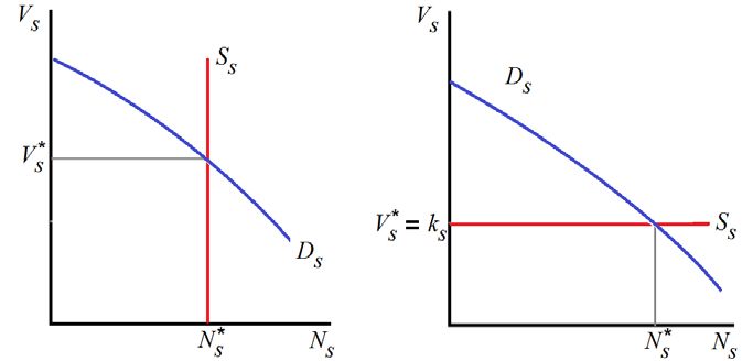
mapping environments into outcomes. While there is not complete consensus on
usage, we take a stand: competitive search equilibrium means that agents on one
side of the market post the terms of trade, while agents on the other side observe
what is posted and direct their search accordingly. This can be applied in environ-
ments with finite or infinite numbers of agents; the situation where these numbers
are sufficiently large that certain strategic considerations can be ignored is called
perfectly competitive search equilibrium.
       Consider any two-sided market with, e.g., buyers and sellers, firms and workers,
or borrowers and lenders, trying to get together in pairs. Traditional search assumes
they meet exogenously, at random, although whether a meeting results in trade can
be endogenous. Directed search is different because agents use the information to
target their search towards particular types, and sometimes even particular indi-
viduals. This can be based on primitive characteristics of agents — e.g., buyers can
search for sellers of particular good — and on endogenous characteristics like the
posted terms of trade. In competitive search equilibrium resources are allocated
through the terms of trade plus the probability of trade. This is distinct from Wal-
rasian theory, where trading probabilities play no role, and from traditional random
search models, where prices have a relatively minor allocative role.3 Competitive
search thus integrates elements of GE (general equilibrium) theory and traditional
search theory, yet is still tractable and often delivers clean results.
       Further, in terms of realism, Howitt (2005) puts it like this: “In contrast to
what happens in [random] search models, exchanges in actual market economies are
organized by specialist traders, who mitigate search costs by providing facilities that
are easy to locate. Thus when people wish to buy shoes they go to a shoe store; when
hungry they go to a grocer; when desiring to sell their labor services they go to firms
known to offer employment. Few people would think of planning their economic
lives on the basis of random encounters.” Even more colorfully, Hahn (1987) says
“someone wishing to exchange his house goes to estate agents or advertises — he
does not, like some crazed particle, wait to bump into a buyer.” And Prescott
   3
     As Hosios (1990) says about labor, “Though wages in bargaining models are completely flex-
ible, these wages have nonetheless been denuded of any allocative or signaling function: this is
because matching takes place before bargaining and so search effectively precedes wage-setting...
In conventional market situations, by contrast, firms design their wage offers in competition with
other firms to profitably attract employees; that is, wage setting occurs prior to search.”

                                               2
(2005) says “I think the bilateral monopoly problem has been solved. There are
stores that compete. I know where the drug store and the supermarket are, and I
take their posted prices as given. If some supermarket offers the same quality of
services and charges lower prices, I shop at that lower price supermarket.”
Whether or not they realize it, while attempting to critique traditional search
theory, these commentators with their pithy remarks are all describing facets of
directed or competitive search. Our view is that there is a role for random matching
models, with bargaining or other means for determining the terms of trade, but it
is also good to know the alternatives. The models presented below provide a class
of alternative that is becoming increasingly popular and has proved useful in many
applications. After discussing details of the various models and applications, we will
say more about the advantages and disadvantages of the alternative approaches.
We present models of finite markets and limiting results for large markets. In
all of these models frictions take center stage, even when the set of agents is large.
In particular, some sellers can have few customers, while others have more than
they need, leading to rationing, unsold inventories, the coexistence of vacancies and
unemployment, etc. The theory captures a powerful idea: if you post more favorable
terms, customers may come to you with a higher probability, but not necessarily
with probability 1. If a restaurant only has a certain number of tables, or a firm only
wants to hire a certain number of workers, it may not be smart to go where everyone
else is going. These kinds of capacity constraints play a major role in the models
surveyed below, and mean that agents must consider both the terms of trade and
the probability of trade. Of course capacity also matters in GE theory, but only at
the market level — one cannot ask about the capacity of an agent’s trading partner,
because the agent trades with the market and not with each other.
The paper is organized as follows. Section 2 starts with static models, one
framed in terms of goods and one in terms of labor markets. Section 3 embeds
these in dynamic GE to discuss the time to execute trades (e.g., how long an unem-
ployed worker or unsold house remains on the market), as well as endogenous price
dispersion and stickiness. Section 4 presents applications in monetary economics,
where the framework provides a very natural approach. While Sections 2-4 use
large numbers of agents, Section 5 analyzes finite markets and then takes limits as
3the market gets large. Section 6 studies heterogeneity and sorting. Sections 7 and
8 consider private information and mechanism design. Sections 9 and 10 mention
other topics and conclude. In general, applications that do not pique a reader’s
interest can be skipped without loss of continuity. As a rule of thumb, footnotes
contain optional material (e.g., additional citations or technical details) and can also
be skipped without loss of continuity. Appendices as usual can be skipped, too, but
they contain some new or hard-to-find technical material that is potentially useful.4
2 Benchmark Models
2.1 Goods Markets
Consider a market with large numbers of two types of agents, called buyers and sell-
ers, with measures and , and let = denote the population buyer/seller
ratio. One can think of buyers as households, or consumers, and sellers as retailers,
but other interpretations are possible (e.g., producers buying inputs from suppliers).
There are two tradable objects. There is an indivisible good , and sellers can pro-
duce exactly one unit at cost ≥ 0, while buyers want to consume exactly one unit
for utility ; and there is a divisible good that anyone can produce at cost
() = and consume for utility () = . The idea is that there are gains from
trade in , while serves as a payment instrument that buyers use to compensate
sellers. This can be interpreted as direct barter, although more typically in the
literature it is called transferable utility.5
For now each seller simply posts a price , the amount of buyers must pay
to get . Each buyer directs his search after observing all posted prices (all we
actually need is that each buyer observes at least two prices; see Acemoglu and
Autor 2016, Theorem 13.4). Suppose traders meet pairwise. Thus, if a set of buyers
with measure direct their search toward a set of sellers with measure , the
probability a seller meets a buyer is = (), where = is the buyer/seller
4
While there is no previous survey on directed search, some surveys on labor, money, housing
and IO touch on it, e.g., King (2003), Rogerson et al. (2005), Shi (2008), Han and Strange (2015),
Lagos et al. (2017) and Armstrong (2017). We try to provide an integrated framework.
5
Sometimes is called money or numeraire, but that is very bad language. It should be obvious
that it is not really money (below we discuss genuine money). It is also not numeraire, which is
the good with price set to 1 in the Walrasian budget equation, because there is no budget equation
in this model (below we consider models with genuine numeraire goods).
4ratio, also called the queue length or market tightness. Similarly, the probability
a buyer meets a seller is = () . It is standard to assume = () is
increasing and concave, which implies = () is decreasing, given the natural
restriction (0) = 0. In static or discrete-time models and are probabilities, so
we impose 0 ≤ ≤ 1; in continuous-time they are arrival rates, so we only impose
≥ 0. We also usually assume differentiability, and sometimes lim→0 0 () = ∞.
To understand this, imagine any two-sided market with 1 and 2 agents on each
side, where the number of bilateral meetings between types 1 and 2 is = (1 2 ).
Analogous to a production function mapping inputs into output, is assumed to
be increasing and concave, and usually to display CRS (constant returns to scale).
Then 1 = (1 2 ) 1 = ( 1) , where = 1 2 , and 2 = (1 2 ) 2 =
( 1). This generalizes models of one-sided markets (e.g., Diamond 1982), and is
more interesting because the ’s depend on tightness, even with CRS. In addition,
with a two-sided specification it is natural to endogenize tightness by allowing entry
by one side. For now, a buyer seeks a seller with a particular , but whether he
finds one is random (in Section 5 an agent finds a counterparty for sure, but may
or may not trade, due to capacity constraints).
A set of sellers posting the same and buyers searching for them constitutes a
submarket with tightness = . Thus, a submarket is characterized by ( ).
Buyers and sellers payoffs are denoted and . Sellers maximize by posting
( ), although it is not crucial that they post — sellers can equivalently post only
and let buyers work out the equilibrium for themselves. In any case, for a seller
to be in business, ( ) must deliver to buyers their market payoff , which is an
equilibrium object, but taken as given by individuals. This is called the market
utility approach.6
Then sellers solve the following problem:
()
= max () ( − ) st ( − ) = (1)
Sellers’ payoff in a submarket is their trading probability times the surplus = −,
and buyers’ payoff is their trading probability times the surplus = − . While a
6
Early use of this approach includes, e.g., Montgomery (1991), McAfee (1993), Shimer (1996)
and Moen (1997); Peters (2000), based on Peters (1991), derives it from microfoundations, as do
Julien et al. (2000) and Burdett et al. (2001), as discussed in Section 5.
5more rigorous definition of competitive search equilibrium appears in Section 6, the
idea is basically optimization and market clearing: sellers maximize subject to
buyers getting ; and the emerging from (1) is consistent with the set of buyers
and sellers in the market. Notice sellers can get the same from lower if is
higher, and buyers can get the same from higher if is lower. These trade-offs
are a quintessential element of the theory.
To solve (1), use the constraint to eliminate in the objective function:
= max { () ( − ) − } (2)
This problem has a unique solution.7 If it is interior it satisfies the FOC 0 () ( − ) =
. Then, given , the constraint yields uniquely, so any active submarkets must
have the same ( ). Hence, given CRS, we only need one submarket.
There are two standard ways to proceed. The first is to assume and are
fixed. Then the equilibrium buyer-seller ratio must be the same as the population
ratio, = (market clearing). The FOC then implies = 0 () ( − ), and the
constraint implies = − (), or
= + (1 − ) (3)
where = () ≡ 0 () () is the elasticity of () wrt tightness. Hence, price
is a weighted average of cost and utility that splits the ex post (after meeting) surplus
= − according to = ( − ) and = (1 − ) ( − ). The ex ante (before
meeting) payoffs can now be written = ( − ) and = (1 − ) ( − ).
This uniquely pins down the equilibrium h i.
The second way to proceed is to assume one side has a cost to participate, and
therefore, in general, only some of them enter the market. Suppose it is sellers that
have a participation cost . Then in equilibrium, as long as is neither too big
nor too small relative to , some but not all sellers enter, and we have the free
entry condition = . As above, the FOC implies = 0 () ( − ) and the
constraint implies = + (1 − ) . Now = = () ( − ), from which we
get . Once again these conditions uniquely pin down h i.
7
Appendix A proves this in a generalized verion without transferable utility: if a buyer makes
payment to a seller, the latter gets () while former gets − (); in the text here () = () =
. In fact, what is shown is that the SOC’s hold at any solution to the FOC’s, so if there is an
interior solution it is unique, but one should also check for corner solutions.
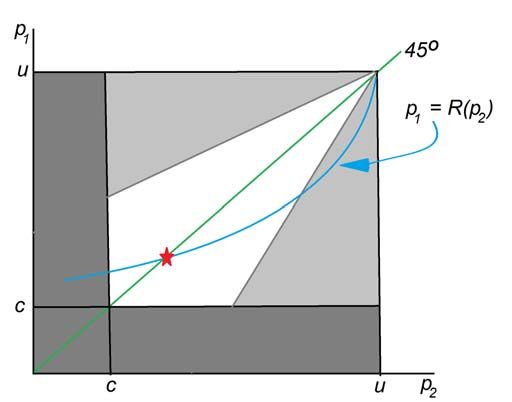
6Figure 1: Equilibrium with (right) and without (left) entry by sellers
Fig. 1, a version of which appears in Peters (1991), shows the “Edgeworth box”
in ( ) space. Indifference curves for buyers slope down, because they are willing
to pay higher if is lower, so they can trade faster. Similarly, sellers are willing to
accept lower if is higher. As in elementary microeconomics, efficient outcomes
are points of tangency, tracing out the contract curve C. The left panel depicts the
case without entry, where C crosses = ; the right depicts the case with entry by
sellers, where C crosses the indifference curve = .
For comparison, consider this problem
()
= max ( − ) st () ( − ) = (4)
where it looks like buyers post and sellers search. It yields the same h i as
(1), with fixed or with entry. One can also consider a third version, with third
parties, called market makers, designing submarkets by posting ( ) to attract
buyers and sellers (see Moen 1997 and Mortensen and Wright 2002 for more discus-
sion). Again the outcome is the same. Hence, it does not matter if buyers, sellers
or market makers post here (this is not always true; see below).
Fig. 2 describes competitive search equilibrium by depicting the solution to (4)
as a “demand” for sellers as a function of the “cost” (given , choosing
is the same as ). One can check “demand” is decreasing and, as shown, hits 0
at finite . Without entry, in the left panel “supply” is vertical and equilibrium
determines . With entry by sellers, in the right panel “supply” is horizontal at
and equilibrium determines . Indeed, one could nest these with a general upward-
7Figure 2: Equilibrium with (right) and without (left) entry by sellers
sloping “supply” curve by letting vary with the number of homogeneous entrants,
or across heterogeneous potential entrants. The point of Fig. 2, like Fig. 1, is that
the theory can be described using tools from elementary microeconomics.
Now consider a planner’s problem with endogenous participation by sellers,
½ ¾
()
max ( − ) − (5)
The first term is the expected surplus per buyer; the second is the total entry cost
of sellers per buyer, since = 1. If we eliminate from the objective function
in (4) using the constraint, this is the same as (5). Hence, equilibrium is efficient.
For yet another comparison, consider bargaining instead of posting.8 Thus, after
a buyer and seller meet, they determine by generalized Nash bargaining,
max ( − ) ( − )1− (6)
where is buyer bargaining power. The solution is = + (1 − ) , which is the
same as under posting, and hence efficient, iff = . This is the well-known Hosios
(1990) condition: efficiency obtains iff agents’ bargaining powers are equal to the
elasticity of the meeting technology wrt their participation.9 Hence, sellers should
8
The easiest interpretation is that there in no communication outside of meetings, so agents
cannot post terms to attract counterparties. Another is that it agents cannot commit to what
they post, although that need not mean it is irrelevant (Menzio 2007; Doyle and Wong 2013; Dutu
2013; Kim and Kircher 2015; Stacey 2016a,b).
9
Earlier discussions of efficiency in related models include Mortensen (1982a,b) and Pissarides
(1986). More recently, Mangin and Julien (2016) show this: with one-side heterogeneity, on the
side searching, several environments generate an expected trade surplus that endogenously depends
on tightness; they derive a generalized Hosios condition that implements (usually) efficiency by
trading off the probability of trade with not only the terms of trade, but also the expected surplus.
8get a share of − commensurate with their contribution to matching. Since this is
exactly what competitive search delivers, it is often said that it induces the Hosios
condition endogenously.
If = is fixed, one can check 0 and 0, while ≈
−0 where “ ≈ ” means “ and have the same sign.” Now 0 0, and hence
0, for many common meeting technologies, but not all.10 Does 0
make sense? Yes. First note that higher always increases and decreases ,
where these can change due to either changes in or in the trading probabilities.
By construction () goes up and () down with , but if they move a lot,
must go down so the changes in and are not too big. Hence an increase in
demand along the extensive margin (higher ) can lower , although one can show
an increase along the intensive margin (higher ) implies 0 unambiguously.
Similarly, with seller entry, higher reduces and raises , also implying ≈
−0 and 0. That might fall when the buyer-seller ratio rises reflects the
idea that resource allocation is guided by both prices and probabilities.
2.2 Labor Markets
Now let households be sellers, of their time, and firms buyers. Each firm wants to
hire exactly one worker, while each household wants to land one job. Thus, is the
vacancy-unemployment ratio. Again, it does not matter here who posts and who
searches. Consider a version of (1) that maximizes workers’ payoffs,
()
= max () ( − ) st ( − ) = (7)
where is output per worker and is the value of unemployment benefits, leisure
and home production sacrificed by taking a job. Here , and play the roles of
, and in the goods market.
Emulating Section 2.1, with = fixed, we get = + (1 − ) , =
(1 − ) ( − ) and = ( − ). And with entry by buyers (the firms in this
application), we get a similar outcome except is endogenous and = . With
= fixed we have ≈ −0 , and with entry we have 0 and
10
Appendix E shows 0 () ≷ 0 ⇔ () ≷ 1, where () is the elasticity of substitution.
Consider a CES technology, (1 2 ) = (1 + 2 )1 , ∈ (−∞ 1), where = 1 (1 − ). Then
0 ⇒ 0 0, 0 ⇒ 0 0, and, in the Cobb-Douglas case, = 0 ⇒ 0 = 0. The point is
that it is not hard to get 0 0 and hence 0 in examples.
9 ≈ 0 . If 0 0 then goes up when with tightness, as one might expect,
but that is not true in general, as explained above for goods markets. As other
features of goods markets also carry over, we proceed to applications.
Albrecht et al. (2006), Galenianos and Kircher (2009) and Kircher (2009) let
workers apply for more than one job.11 If workers can apply to ∈ {1 2 } vacan-
cies, then it turns out there will be distinct wages posted, and the optimal search
strategy is to apply to one of each — i.e., to look for work simultaneously in distinct
submarkets. Hence, the model exhibits wage dispersion with homogeneous agents,
as is relevant because a large part of empirical wage variation cannot be explained
by observables (Abowd et al. 1999; Mortensen 2003). Also, consistent with the ev-
idence, the density of posted wages can be shown to be decreasing, while by way
of contrast, in models based on Burdett and Mortensen (1998), with homogeneous
agents the density is increasing. Also, again consistent with conventional wisdom,
firms offering higher wages receive more applications.
Allowing multiple applications introduces an element of portfolio choice for work-
ers, with low-wage applications serving to reduce the downside risk. This embeds
in an equilibrium setting a version of Chade and Smith’s (2006) marginal improve-
ment algorithm. For a simplified exposition, consider = 2, so there are two wages
posted, 1 and 2 ≥ 1 , with workers sending applications to two distinct submar-
kets. If both pan out, they accept the highest wage; if only one pans out, they take
it. Their expected payoff is therefore
= max {(2 )(2 − ) + [1 − (2 )] (1 ) (1 − )} (8)
1 2
where is the tightness in a submarket posting .
Generalizing the above methods, in the low-wage submarket, we solve
[1 − (1 )] (1 )
1 = max (1 )(1 − ) st ( − 1 ) = (9)
1 1 1
where () is the probability a worker rejects 1 if offered. Given a solution to (9),
substitute 1 into (8) to obtain the problem for the high-wage submarket
(2 )
= max {(2 )(2 − − 1 ) + 1 } st ( − 2 ) = (10)
2 2 2
11
One difference is: in Albrecht et al. (2006), if two or more firms make offers to the same worker
they compete à la Bertrand (see also Albrecht et al. 2003,2004); as in Galenianos and Kircher
(2009) or Kircher (2009), here firms commit to posted wages.
10This looks like a problem with = 1, but now the outside option is + 1 , not
just . Since a higher outside option raises the posted wage, this is consistent with
2 1 . Thus we support 2 posted wages.
For efficiency, in Galenianos and Kircher (2009), a worker who gets a high wage
still enters the queue at low wages. With = 2, if a fraction of firms post 1 then
1 = , 2 = (1 − ) and (1 ) = (2 ). To characterize equilibrium,
solve (9) and (10) with set so that is the same in the two submarkets. The
outcome is inefficient. Since workers obtaining jobs at 2 still enter the queue at
1 , they can prevent others from getting 2 . Neither the firms posting high wages
nor the workers who obtain them take this into account, implying an unpriced
externality. In Kircher (2009), workers who obtain 2 no longer queue for 1 . This
implies (1 ) = 0 since any worker in the low-wage queue does not have a high-wage
offer. This achieves efficiency since the unpriced externality disappears.12
2.3 Summary of Baseline Models
Table 1 provides comparative statics for goods and labor markets in the benchmark
model, where agents can only search in one submarket, for three cases: (a) fixed
populations; (b) entry by sellers; and (c) entry by buyers. Most results are unam-
biguous, except as explained above some of the effects on or can go either way.
A few cases report +∗ or −∗ to indicate the signs are ambiguous, in general, but +
or − in the common case 0 ≤ 0.
The analogous table for bargaining is similar, except effects reported as 0 or
−0 would be 0, and those reported as +∗ and −∗ would be + and −. The models
above have those results in the special case of a Cobb-Douglas meeting technology,
where 0 = 0, but in general parameters that affect can move trading probabilities
enough to move prices in ways that are counterintuitive without understanding the
theory. Under bargaining the terms of trade do not change with , because while
12
As a referee said, it is not clear how to compare the results because one can say the environment
is different if workers who obtain 2 no longer queue for 1 . In any case, the main point here is to
say that efficiency models depends on details. Wolthoff (2014) constructs a model encompassing
Kircher (2009) and Galenianos and Kircher (2009), endogenizes firms’ recruitment effort, and
concludes that multiple submarkets are crucial for matching the data. Gautier and Holzner (2016)
introduce a more sophisticated process to bid for workers after matching, so no vacancies remains
idle because workers reject them to join firms with more applicants than they need, and that leads
to efficiency. All this work constitutes progress, but there is still room for more.
11arrival rates affect expected payoffs, they do not affect the surpluses after traders
meet, and hence are irrelevant in the negotiations. Now in dynamic models, as
discussed below, can affect continuation values and hence the bargaining outcome,
but in competitive search equilibrium affects the terms of trade even in a static
environment. In any case, we highlight the following results:13
Proposition 1 In the benchmark model, with homogeneous agents that can search
in at most one submarket, with or without entry, there is a unique equilibrium and
it has a single price or wage. This is efficient. When agents can simultaneously
search in 1 submarkets, there is a unique equilibrium and it has prices or
wages. This is efficient if there are no unpriced externalities.
Table 1.1: Goods Market Table 1.2: Labor Market
(a) = fixed (a) = fixed
+ −0 − + 0 −0 + −0 − + 0 −0
0 + + + + + 0 + + + + +
0 + − − − − 0 + − − − −
(b) entry by sellers (firms) (b) entry by sellers (households)
+ −0 − + 0 −0 + −0 − + 0 −0
− + + 0 +∗ + − + + 0 +∗ +
+ +∗ − 0 −∗ − + +∗ − 0 −∗ −
(c) entry by buyers (households) (c) entry by buyers (firms)
− 0 + − −0 0 − 0 + − −0 0
+ +∗ 0 + + +∗ + +∗ 0 + + +∗
− + 0 − −0 −∗ − + 0 − −0 −∗
3 Extensions and Applications
It is desirable to consider dynamics models, where meeting probabilities translate
into random durations between trades. For goods markets, we can simply repeat the
static version, and since that is easy we add a few other features. Simply repeating
a static model is less natural for labor, so we incorporate long-term relationships.
13
As a referee pointed out, some of our Propositions are really just summaries of discussions in
the text. Others are more rigorous and have nontrivial proofs. At the risk of appearing pretentious,
we label them all as Propositions, mainly to maintain symmetry in the way we highlight key aspects
of the presentation.
123.1 Goods Markets
The markets studied above can be embed in dynamic GE using the structure in
Lagos and Wright (2005): Each period in discrete time, agents interact in two
ways: in a decentralized market, or DM, like the one analyzed above; and then in a
frictionless centralized market, or CM.14 Continue to let and be the DM value
functions, and now let and be the CM value functions. In the CM, buyers
solve
() = max { () − + } st = − (11)
where is the discount factor, is CM numeraire, is labor, is the wage and is
debt from the previous DM.15 To ease notation, assume is produced one-for-one
with , so that in equilibrium = 1. Then the solution to (11) has = ∗ where
0 (∗ ) = 1. Also, the envelope condition is 0 () = −1. The CM problem for
sellers is omitted, but similar.
For buyers, the DM payoff is
= [ + ()] + (1 − ) (0) = ( − ) + (0) (12)
because () − (0) = −, by the envelope condition. Similarly, for sellers
= ( − ) + (0) (13)
Except for (0) and (0), notice and are identical to the static model.
Hence, making the benchmark dynamic in this way is easy, but still nice, since higher
() now means sellers trade faster, mapping neatly into the realm of duration
analysis as used in much empirical work (e.g., Devine and Kiefer 1991). In particular,
the expected times for sellers and buyers to transact are 1 () and ().
14
There are several appealing aspects to this alternating CM-DM structure: First, we can dis-
pense with buyers paying in the DM using transferable utility, and have them pay in terms of
numeraire in the next CM (and there is a genuine numeraire here, in contrast to the situation in
fn. 5) Also, we can make credit imperfect to analyze debt limits and money in serious ways. Also,
precisely for these reasons, this is now the workhorse model in monetary theory, and we want to
use it in 4.2 below. Moreover, it is a tractable way to integrate search into general equilibrium,
which lets one add markets for capital, other assets, etc. In fact, adding the CM actually simplifies
rather dramatically the analysis of models with only DM trade. But it is not just a way to simply
things, we think it is realistic: some aspects of one’s actual economic live are well modeled by
frictionless or centralized trade; others seem better captured by search or decentralized trade; and
it seems good to have a setup with some of each. See Lagos et al. (2017) for more.
15
One-period debt is without loss of generality, given quasi-linear CM utility, although we can
2
generalize to any utility function satisfying 11 22 = 12 (see Wong 2016).
13Figure 3: Heterogeneous buyers (left) or sellers (right)
While heterogeneity is covered more fully in Section 6, it is worth seeing some
examples here. Consider two types of buyers with utilities 1 and 2 1 , and entry
by homogeneous sellers. Then the market segments into two distinct submarkets,
= 1 2, where ( ) is determined by
= [ ( ) − 0 ( )] ( − ) and = + ( ) (14)
Notice (14) holds for = 1 2 independently, a feature called block recursivity. It lets
us first solve for in each submarket (block 1) regardless of what is happening
in other submarkets; then the number of agents in each submarket is determined
(block 2) so the total number of buyers sums to the number in the economy, and
free entry of sellers ensures market tightness is correct (more on this below).
Given 2 1 , one can check 2 1 and 2 1 . Thus, high-valuation buyers
go to submarket 2, where they pay more but trade faster. Sellers trade slower in
submarket 2 and, in equilibrium, they are indifferent between it and submarket 1.
This is shown in the left panel of Fig. 3, with buyers in submarkets 1 and 2 on
indifference curves denoted 1∗ and 2∗ , both of which are tangent to the sellers’
common indifference curve ∗ = .
Now consider homogeneous buyers and two seller types in fixed numbers 1 and
2 , with 1 and 2 1 but the same (Julien et al. 2006a consider different ).
Suppose is not too big, so all sellers participate. As shown in the right panel of
Fig. 3, the market segments into two submarkets where now buyers are indifferent
14between them. As usual, ( ) is determined by
0 ( ) ( − ) = and = ( ) + [1 − ( )]
Let us normalize = 1 and let be the fraction of buyers in submarket 1. Then
buyer indifference uniquely determines by
µ ¶ µ 
0 0 1−
( − 1 ) = ( − 2 )
1 2
One can check 2 1 and 2 1 , so sellers in submarket 2 trade slower, while
buyers trade faster but pay higher prices.
Clearly the theory accommodates deviations from the law of one price. With
heterogeneous buyers, sellers in submarket 1 settle for 1 , even though others are
getting 2 1 , because the latter take longer to sell. With heterogeneous sellers,
buyers in submarket 2 pay 2 even though others are paying 1 2 , for similar
reasons. This is related to yet different from other theories of price dispersion. In
Burdett and Judd (1983), e.g., buyers see a random number of prices simultaneously
— called noisy search — and when they see more than one they pick the lowest. In
equilibrium ex ante identical sellers post different prices but earn equal profits, as
those with lower earn less per unit but make it up on the volume. That is like our
sellers, but Burdett-Judd buyers do not make a directed choice between paying less
or trading faster the way they do here.
Returning to heterogeneous buyers and homogeneous sellers, consider the appli-
cation to housing in Rekkas et al. (2017). There are a fixed number of homogeneous
houses in the market, but buyers are heterogeneous, with the value to becoming a
home owner distributed continuously across buyers with CDF () and support
[1 2 ]. Now equilibrium involves a continuum of submarkets indexed by ( )
(this is treated more formally below). Hence there is a submarket for every point
on sellers’ common indifference curve between (∗1 ∗1 ) and (∗2 ∗2 ), with higher
associated with higher and lower . Higher-valuation buyers search where their
trading probabilities and prices are higher, while sellers are indifferent because list-
ing a house at a higher price means a longer average time on the market. Of course,
it is no surprise that a big home in a nice neighborhood costs more than a small
one in a bad neighborhood; the interest here is in residual price dispersion, the way
labor economists are interested in residual wage dispersion.
15What may be less obvious is the model is consistent with sticky prices. If market
conditions change, the distribution reacts, but if the change is not too big the old and
new supports overlap, and sellers with in the overlapping range have no incentive
to reprice. If demand falls, e.g., the distribution shifts left, but many sellers can
keep the same . This is relevant because people claim house prices are sticky in
the data and find it puzzling: “conventional wisdom is that traditional, rational,
forward-looking economic theories are unable to explain extreme price stickiness of
this sort, unless there are large menu costs” (Merlo et al. 2015). More generally,
directed search is natural for understanding many aspects of housing markets.16
Moving from houses back to generic goods, let us now make them divisible:
DM buyers get a quantity or quality in exchange for payment in the next CM.
Buyers’ utility and sellers’ cost, () and (), satisfy the usual properties, plus
(0) = (0) = 0 and (̄) = (̄) for some ̄ 0. The efficient solves 0 ( ∗ ) =
0 (∗ ). One can call ̂ = the unit price, unless is unobserved quality, in which
case one might still call the price. We assume both and are posted, although
there are alternatives — e.g., perhaps due to limited commitment, there may be a
posted unit price ̂, and then in a meeting is chosen unilaterally by the buyer
(Peters 1984) or the seller (Gomis-Porqueras et al. 2017).
We also introduce a limit on how much one can promise to pay, ≤ , a
debt/liquidity constraint that is exogenous for now, but endogenized in Section 4.
If it is slack then, ignoring the constants (0) and (0), we have
()
= max [() − ] st () [ − ()] = (15)
Indeed, when ≤ is slack, the solution has = ∗ , so the problem is basically
the same as the one with a fixed , and the usual procedure yields (∗ ∗ ). The
generalization of (3) is ∗ = (∗ ) (∗ ) + [1 − (∗ )] (∗ ), and the constraint is
16
In Albrecht et al. (2016), sellers first list prices, with more attractive prices meaning more
buyers show up on average (although the actual number is random, as in Section 5). Each buyer
can accept the listed price or make a counteroffer. If no buyers accept, the seller can accept or
reject the best counteroffer. If exactly 1 buyer accepts, he gets the house at the listed price. If 2
or more accept, the seller runs an auction. This is consistent with data showing that houses can
sell at, above or below listed prices. In other applications, Diaz and Jerez (2013) build a model
consistent with cyclical data. Head et al. (2015) have heterogenous sellers, and highly-indebted
home owners tend to list high prices and take longer to sell. Hedlund (2015) has heterogenous
buyers and sellers and accounts for cyclical dynamics. See also Hedlund (2016), Garriga and
Hedlund 2016), Stacey (2015a), Moen et al. (2016) and Head at al. (2017).
16indeed slack iff ≥ ∗ .
When ∗ , so the constraint binds, the results are quite different. In Appendix
A we solve (15) and show the SOC’s hold at any solution to the FOC’s, so there is
a unique interior solution, and it implies = ( ) where
() 0 () () + [1 − ()] 0 () ()
( ) ≡ (16)
() 0 () + [1 − ()] 0 ()
This condition appears in many models with liquidity considerations and Nash bar-
gaining (see Section 4), except () replaces buyers’ bargaining share . More com-
plicated versions of this setup are studied by Rocheteau and Wright (2005), Menzio
et al. (2013) and Choi (2015). We again highlight the main results as follows:
Proposition 2 Dynamic models with credit yield results analogous to static models
with transferable utility, with endogenous and fixed, or vice versa. Heterogeneity
segments submarkets by probability and price. Price stickiness emerges as follows:
when market conditions change, some prices can stay the same, as endogenous trad-
ing probabilities make some agents indifferent to changing posted terms.
3.2 Labor Markets
While enduring relationships may be relevant in goods markets — one may have a
favorite shop or bar — in labor markets they are ubiquitous. We now work through
Moen (1997), a directed search version of Pissarides (2000), where market tight-
ness is = (1 − ), the measure of vacancies over unemployment, and is the
employment rate with a population of households normalized to 1.
Here we use continuous time.17 Then letting 1 and 0 be firms’ payoffs to
having a worker and an open vacancy, in steady state we have
()
0 = − + (1 − 0 ) (17)
1 = − + (0 − 1 ) (18)
where is the cost of a vacancy, the discount rate, and the job destruction rate
(which is exogenous, but can be endogenized as in Mortensen and Pissarides 1994).
In words, e.g., (17) says the flow payoff to a vacancy is − plus the arrival rate
17
There is no CM in this environment, but it can be interesting to add one (Berentsen et al. 2011;
Gomis-Porqueras et al. 2013; Zhang and Huangfu 2016; Dong and Xiao 2016).
17of workers, () , times the gain to filling the position, 1 − 0 . Similarly, for
households
0 = + () (1 − 0 ) (19)
1 = + (0 − 1 ) (20)
Again it does not matter for results if firms or workers post, but the latter is
easier, since 0 = 0 (free entry) combined with (17)-(18) yield
= − ( + ) () (21)
Solving (17)-(18) for 0 and inserting from (21), the relevant problem is
() ( − ) − ( + )
0 = + max
+ + ()
The FOC implies () = 0, where
() ≡ 0 () ( − ) − [ + + () − 0 ()] (22)
and one can check (0) 0 (∞) and 0 () 0.
So there is a unique solution to () = 0, and hence a unique equilibrium .
One can derive
0, 0, 0, 0 and 0 (23)
The effects of , and are consistent with Table 1.2(c), plus there are new effects
of and , and all accord well with intuition. One can also show 0,
0 and 0, plus 0 and 0 if 0 ≤ 0.
Appendix B shows the equilibrium outcome is the same as the solution to a
planner’s problem posed without restricting attention to steady state — i.e., the
efficient solves () = 0 at every date, as in Pissarides (2000). This is again
block recursivity, where the measure of vacancies depends on , but tightness
= (1 − ) does not. Rearranging () = 0, we get
() () ( − )
= (24)
+ + () [1 − ()]
which equates firms’ vacancy cost to their arrival rate times their share, (), of
the appropriately-discounted surplus − . This is the same as Pissarides (2000),
18except the elasticity replaces firms’ bargaining share . It matters: if we change
labor-market policy, e.g., as long as 0 () 6= 0 the effects are different than predicted
by bargaining.
Extensions allowing on-the-job search include Moen and Rosen (2004), Delacroix
and Shi (2006), Garibaldi and Moen (2010), Schaal (2015), Tsuyuhara (2016) and
Garibaldi et al. (2016). Among other reasons, this is interesting because data show
there are many direct job-to-job transitions (Fallick and Fleischman 2001; Chris-
tiansen et al. 2005). As in Delacroix and Shi (2006), let 0 be workers’ cost
of search while employed, assumed small enough that at least some workers search
while employed. This generates wage dispersion. Let () be the ratio of vacancies
to job seekers in a submarket with wage . The problem of a worker employed at
is
1 () = + [0 − 1 ()] + max
0
Σ{ [(0 )] [1 (0 ) − 1 ()] − } (25)
Σ
where Σ = 1 (Σ = 0) indicates he engages in (abstains from) search, and if Σ = 1
then 0 is the next wage to which he directs his search.
An unemployed worker’s value function is similar to a worker employed at = ,
except it is assumed that the former has no search cost, so 0 = 1 () + . Also,
workers are more selective in terms of the next targeted wage 0 when their current
wage is higher (see Appendix C). Solving for equilibrium requires finding ().
To begin, write
[()]
0 = − + [1 () − 0 ]
()
1 () = − + [ + ()] [0 − 1 ()]
where the only change from the baseline model is that jobs now end with an exoge-
nous probability plus the endogenous probability () that a worker gets a better
offer. Now free entry implies 0 = 0, or
[()] −
= (26)
() + + ()
Then 0 implies there is a such that workers employed at ≥ naturally
stop searching. For firms paying ≥ , () = 0, and (26) identifies the () that
coincides with what one gets without on-the-job search.
19Under the hypothetical situation that () is computed this way everywhere, we
can find the lowest wage at which the solution to (25) involves no search, and that
identifies . Then, by way of induction, notice there is a minimum wage increment
4 that workers require to justify search (Appendix C). Hence, those employed at
∈ [ − 4 ) only seek jobs with 0 ≥ , for which we have already determined
(0 ). Given , 0 is the unique solution to (25), denoted 0 = (). Then
() = ◦ ◦ (), where for any functions and , ◦ () denotes the composite
[ ()]. Knowing () ∀ ∈ [ − 4 ), entry condition (26) yields () at these
wages. Repeating the procedure for ∈ [ − 24 − 4) yields () and () at
those wages, and so on, until () and () are determined for all .
This establishes () and () ∀ without reference to the distribution of
employment across , in and out of steady-state, again due to block recursivity.
Starting with higher unemployment, e.g., lots of job seekers search for = (),
but also lots of firms post = (), keeping () as determined above. Thus,
we can first solve for the value functions and decision rules (block 1), then study
the evolution of from any initial condition (block 2), and only in the second step
does the distribution of employment come into play. Extensions of this insight
allow tractable analysis of business cycle models where aggregate productivity
is stochastic. In these models, current is enough to compute tightness in each
submarket, say ( ), which is easier than it would be if depended on the
distribution of ; see Shi (2009), Menzio and Shi (2010,2011), Schaal (2015) and Li
and Weng (2017).
To recap, there are wages, 1 2 . The unemployed apply to
1 = (); workers employed at 1 apply to 2 = (1 ); and so on, until they stop
searching. It can be shown that decreases with search and entry costs. Also,
simple wage contracts do not induce efficiency, similar to the model in Section 2.2
with multiple applications. With on-the-job search, firms care about both recruit-
ment and retention, and a single wage is not sufficient to balance the two. This
is especially clear when all matches produce the same , which means on-the-job
search is rent seeking that has a social cost but does not increase output. However,
more complicated contracts that directly specify search activity, or specify transfers
when workers quit, can restore efficiency (Menzio and Shi 2011).
20Research on labor markets with directed search is a vibrant area. As regards
business cycle fluctuations, in particular, Menzio and Moen (2010) show that the
optimal wage contract with aggregate productivity shocks prescribes rigid wages
for existing workers and downward rigidity for new hires. Menzio and Shi (2011)
exploit block recursivity to develop a tractable model of unemployment, vacancies
and job-to-job transitions over the cycle. In their model, transitions are driven
by heterogeneity in firm-worker matches. They show the labor market’s response
to aggregate shocks is large only if the quality of the match is observed after the
match is created. Schaal (2018) also uses a directed search model to study business
cycles, focusing on the impact of time-varying idiosyncratic shocks at the establish-
ment level. Guo (2018) also uses directed search study recessions in a model with
endogenous schooling and heterogeneous agents.
Proposition 3 The dynamic labor model without on-the-job search has a unique
equilibrium and it is efficient. At each point in time, solves () = 0 and
solves (21). The outcome with on-the-job search is similar, except there is wage
dispersion, and efficiency requires more complicated contracts.
4 Monetary Economics
Monetary theory has used random matching at least since Kiyotaki and Wright
(1989), and that model has been recast using directed search by Corbae et al. (2002,2003).
We present the simple version in Julien et al. (2008), with indivisible assets, then
consider divisible assets.
4.1 Indivisible Assets
£ ¤
A fixed 0 ̄ continuum of ex ante identical agents live forever in discrete time;
there is no entry. Also, there are no centralized markets, as all trade is bilateral,
and that is hindered by specialization: there are many types of goods, and it is
never the case in a pairwise meeting that agent consumes what produces and
vice versa, ruling out direct barter. Assumptions on limited commitment and private
information rule out credit, so that assets have an essential role as media of exchange.
Equal measures of agents consume and produce each good. Everyone has the
same utility () for goods they consume and cost () for those they produce.
21Goods are nonstorable. There is a storable asset that generates utility each period
for anyone holding it: if 0 this is a dividend as in standard asset-pricing theory
(Lucas 1978); if 0 it is a storage cost (Kiyotaki and Wright 1989); and if = 0
the asset is fiat money according to standard usage (Wallace 1980). Individual asset
¡ ¢
holdings are restricted to ∈ {0 1}, so given a fixed supply ∈ 0 ̄ , agents
have = 1 and act as buyers while ̄ − have = 0 and act as sellers.18
A novelty compared to the above models is that after trade the buyer becomes
a seller and vice versa. Letting ∆ = − be the value to getting an asset and
switching from seller to buyer, in steady state we have
= + [ () − ∆] + (27)
= [∆ − ()] + (28)
As usual, = () and = () with = (̄ − ) and () comes from
a general meeting technology, although following Kiyotaki and Wright (1991,1993)
¡ ¢
most papers use = ̄ − ̄.
Directed search plays two roles: first the economy segments into markets trading
different goods; second each market segments into submarkets based on posted
terms. Appendix A shows the FOC’s for the submarket problem lead to
() 0 () () + [1 − ()] 0 () ()
∆ = (29)
() 0 () + [1 − ()] 0 ()
The RHS, denoted ( ) in (16) is again the same as Nash bargaining except ()
replaces ; different from Section 3.1, instead of an exogenous limit , the value of
assets and hence the ability to pay are endogenous.
To proceed, subtract (27)-(28) and solve for
+ () + ()
∆ = (30)
+ +
Then = (̄ − ) determines , and . A stationary monetary equilibrium,
or SME, is then a equating the RHS’s of (29) and (30), with ∈ (0 ̄), with
18
This environment is from Shi (1995) and Trejos and Wright (1995), but those papers use
random search and symmetric bargaining. This is extended to other bargaining solutions by Rupert
et al. (2001) and Trejos and Wright (2016). There are also versions with posting and random search
by Curtis and Wright (2004), or posting and noisy search by Burdett et al. (2016). Wallace (2010)
and references therein use abstract mechanism design. The first paper to use posting and directed
search is Julien et al. (2008), with extensions by Julien et al. (2016) and He and Wright (2019).
22 (̄) = (̄), as required for voluntary trade. In the special but natural case = 0,
one can show there is a unique SME (see He and Wright 2019 for details).
To emphasize the interplay between directed search and monetary economics,
consider the unique SME with = 0, and the meeting technology commonly used
in the literature, with ̄ = 1 and = (1 − ). Then = 12 is good for trade
on the extensive margin, since it maximizes the number of buyer-seller meetings, but
it does less well on the intensive margin, since it implies ∗ . Trejos and Wright
(1995) show ∗ at = 12 using Nash bargaining with = 12. In competitive
search equilibrium, the result ∗ at = 12 follows without restrictions on
because () = 12 holds automatically at = 12. Thus, we get similar results
with fewer conditions, something that is typical of applications using competitive
search theory.
As another connection between directed search and money, consider dynamics.
The model sketched here has nonstationary equilibria for some parameters, where
the value of the asset varies over time, as a self-fulfilling prophecy. That is also
true with Nash bargaining models, but the microfoundations can be criticized in
nonstationary equilibria (Coles and Wright 1998). This critique does not apply to
competitive search, and so one can say it provides a more rigorous model of dynamics
based on liquidity considerations (more on this in Section 9.1). Moreover, monetary
models with competitive search are important in the literature, as early work was
criticized by those who dislike random matching and bargaining. It is thus good to
know that most insights also apply with directed search and posting.
4.2 Divisible Assets
Now let agents hold any ∈ R+ and bring back the frictionless CM convening after
each DM. A nice feature of the CM in this kind of application is that it harnesses the
distribution of , plus it allows one to incorporate many elements of mainstream
macro in search models. Yet another is that we do not have to say whether agents
are buyers or sellers depending on their current as in Section 4.1; instead we can
have some called buyers that always want to consume but cannot produce in the
DM, while others called sellers produce but do not consume. This would not work
with only DM trade.
23Focusing on = 0 buyers’ CM problem is
() = max { () − + +1 (̂)} st = + ( − ̂) − (31)
̂
where is cash brought in, ̂ is cash taken out, is its price in terms of numeraire
, and is a lump sum tax. Other than keeping track of time with the subscript
on +1 (̂), (31) is like (11) with one exception: there buyers get DM goods on
credit due in the next CM; here this is infeasible because of issues with commitment
and information, so buyers need assets as payment instruments. Still, as in Section
3.1 we have 0 () = , so CM payoffs are linear. Sellers do not bring cash to the
0
DM, but buyers may, and their FOC for ̂ 0 is = +1 (̂). Since does not
appear in this FOC, ̂ does not depend on what agents bring into the CM.19
In the current CM, (+1 +1 +1 ) is posted for the next DM, where +1 is the
real value of the monetary payment. Since cash is a poor savings vehicle, buyers hold
just enough so that +1 ̂ = +1 . Again, it may seem natural to have sellers post
and buyers search, but it is equivalent to assume the opposite. Ignoring constants
and time subscripts, after some algebra, we have
½ ¾
()
= max [ () − ] − st () [ − ()] = (32)
where is a nominal interest rate defined by the Fisher equation, 1 + = +1 . In
stationary equilibrium is constant, so inflation is +1 = +1 . This plus
the Fisher equation imply it is equivalent for monetary policy to peg the money
growth, inflation or nominal interest rate.
Problem (32) is the same as (15) but for one detail: buyers now must make an
ex ante investment in liquidity, at cost +1 , before going to the DM. Taking the
FOC for , we get
() = () (33)
where () ≡ [0 () − 0 ()] 0 () is the liquidity premium. The FOC for yields
()
() [1 − ()] [ () − ()] = + (34)
()
19
This history independence, which makes the DM distribution of ̂ across buyers degenerate,
follows from quasilinear utility and the interiority of , but both can be relaxed as discussed in
fn. 15. The distribution is not degenerate in the closely related models of Galenianos and Kircher
(2008) and Dutu et al. (2012), but is still tractable due to history independence.
24You can also read