Does weed control by precision spray technology favour the emergence of resistance?
←
→
Page content transcription
If your browser does not render page correctly, please read the page content below
28. Deutsche Arbeitsbesprechung über Fragen der Unkrautbiologie und -bekämpfung, 27.02. – 01.03.2018 in Braunschweig

Does weed control by precision spray technology favour the emergence of
resistance?
Begünstigt die teilfächenspezifische Unkrautbekämpfung die Entwicklung von Resistenzen?
Otto Richter1*, Roland Beffa2, Dirk Langemann
1Technische Universität Braunschweig, Institut für Geoökologie, Langer Kamp 19c, 38106
Braunschweig, Germany
2Bayer CropScience AG, Frankfurt am Main, Germany
3Technische Universität Braunschweig, Institut Computational Mathematics, Universitätsplatz

2, 38106 Braunschweig, Germany
*Corresponding author, o.richter@tu-bs.de

DOI 10.5073/jka.2018.458.058

Abstract
Weed control by precision farming is recommended both by economic and ecological reasons. It is still unclear
whether precision weed control favours the emergence of herbicide resistant biotypes. To investigate this, the
cellular automaton model of Sandt et al. (2008) for the simulation of precision weed control was extended to
resistant biotypes and their genetic interactions. The model is capable of simulating the emergence of
resistant biotypes in dependence of weed control thresholds, application rates and initial distribution of
biotypes. Examples are shown for the case of polygenic inheritance of resistance involving three loci and thus
27 biotypes. Preliminary simulation results hint that precision farming can delay the emergence of resistance at
high weed control thresholds.
Keywords: Metabolic herbicide resistance, polygenic inheritance, population dynamics, population genetics,
precision agriculture, weed control

Zusammenfassung
Teilflächenspezifische Unkrautbekämpfung ist eine Methode für eine umweltschonende Landwirtschaft. Es ist
jedoch unklar, wie diese Methode die Entwicklung von Herbizidresistenzen beeinflusst. Zur Untersuchung
dieser Fragestellung wurde das von SANDT et al. (2008) für die Simulation der teilfächenspezifischen
Unkrautbekämpfung entwickelte Modell durch die Hinzunahme resistenter Biotypen und ihrer genetischen
Interaktion erweitert. Das Modell ermöglicht die Simulation der Entwicklung resistenter Biotypen in
Abhängigkeit von der Schadschwelle, Aufwandmengen, Fruchtfolgen und der Anfangsverteilung resistenter
Biotypen in der Population. Es werden Beispiele gezeigt für eine polygene Vererbung von metabolischer
Resistenz unter Beteiligung von 3 Loci und damit 27 Biotypen. Erste Simulationsergebnissse deuten darauf hin,
dass teilflächenspezifische Unkrautbekämpfung die Entwicklung resistenter Biotypen verzögern kann.
Stichwörter: Metabolische Herbizidresistenz, polygene Vererbung, Populationsdynamik, Populationsgenetik,
teilflächenspezifische Unkrautbekämpfung

Introduction
In the last decade herbicide resistance has become a major issue for many weeds (BECKIE, 2006;
POWLES et al., 2010). In recent years the adoption of precision farming has been promoted as a
means to reduce herbicide input. Currently, commercial equipment to perform the identification
and spraying of weeds in real time appears on the market, e.g. WEEDit and WeedSeeker. Whereas
the short term economic benefit of site-specific herbicide management seems to be obvious
especially at high weed infestations, the influence of precision farming on the long term
development of herbicide resistance is not quite clear. However, in recent years it has been shown
that low dose application rate favour the emergence of polygenic resistance. There are quite a few
examples such as the evolution of polygenic herbicide resistance in Lolium rigidum by low-dose
herbicide selection (BUSI et al., 2013; YU et al., 2013). So the question arises whether precision
farming might have the same effect on resistance development as low dose application. To this
end a model was developed comprising population genetics and dynamics and dispersal in the
frame of a cellular automaton.

Julius-Kühn-Archiv, 458, 2018                                                                                   389
28. Deutsche Arbeitsbesprechung über Fragen der Unkrautbiologie und -bekämpfung, 27.02. – 01.03.2018 in Braunschweig
Materials and Methods
The model
General structure
A cellular automaton model is set up (cf. Fig. 1). At each grid cell the model comprises a time
discrete population dynamic model of the life cycle of an annual plant with the stages seed (S),
seedling (K), young plant (J) and adult plant (R). Biotypes of different resistance factors are linked
by a genetic submodel. The model allows for both target site and metabolic resistance. Polygenic
inheritance is described by a new approach based on tensor products of heredity matrices (RICHTER
et al., 2016).
Polygenic inheritance
Polygenic inheritance is described by a new approach based on tensor products of heredity
matrices (LANGEMANN et al., 2012). Biotypes with indices i, are ordered lexicographically with
respect to the alleles X j and x j occurring in the gene. Biotype densities c i are combined in a vector
c=(c 1 ,…,c n )t. Rather simple combinatorial investigations in the case of a single gene with n=3
biotypes show that the amount of off-springs is proportional to a quadratic form. Since the
amount of off-springs is related to the rate of change of biotype i, we find c i ’ proportional to ctW i c
with a matrix W i , which is called heredity matrix and elementary heredity matrix in the particular
case of one gene locus. These elementary heredity transmission matrices for the single genes X i ,X j
can be fixed as W i = V i with
1 1/ 2 0
(1)
V1 = 1 / 2 1 / 4 0
0 0
0
0 1/ 2 1
(2)
V 2 = 1 / 2 1 / 2 1 / 2
1 1 / 2 0
0 0 0
(3)
V3 = 0 1/ 4 1/ 2
0 1 / 2 1
and they can be written as the tensor products
V1 = v X ⊗ v tX (4)
V2 = v X ⊗ v xt + v x ⊗ v tX (5)
V3 = v x ⊗ v xt (6)
with
v X = (1 1 / 2 0) t
v x = (0 1 / 2 1) t
390 Julius-Kühn-Archiv, 458, 2018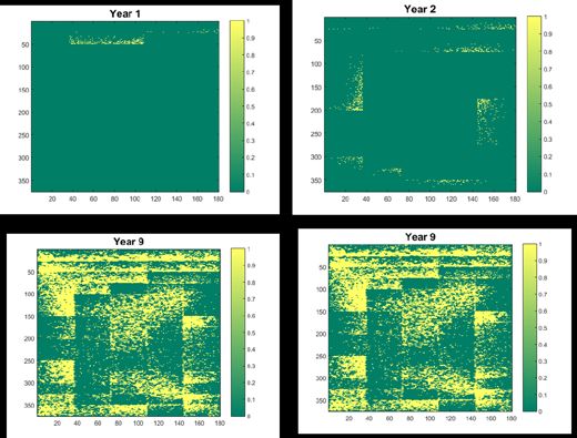
28. Deutsche Arbeitsbesprechung über Fragen der Unkrautbiologie und -bekämpfung, 27.02. – 01.03.2018 in Braunschweig
In the multi loci case transmission matrices W i are obtained from the Kronecker product of the
single transmission matrices
Wi = Vi1 ⊗ Vi 2 ⊗ L ⊗ Vim (7)
with the number m of gene loci and with biotypes ordered again lexicographically with respect to
multiple gene-loci. The reason for the tensor product lies in the fact that inheritance follows
Mendel’s law separately at every gene locus. The fraction of biotype" i" in the population after
random mating is termed normed heredity function and is derived via the hereditary matrices as
c tWi c
g i (c ) = 2
(8)
c sum
Equation (8) gives the rates of off-springs of each biotype and thus, it is the basic for dynamic
population genetic models.
Resistance factors
This general approach is taken from the paper of RENTON et al. (2011). A genotype with n g loci is
presented by the vector
Gt = [ x1 , x2 , x3 ,L xng ] (9)
where xi ∈ [0,1,2] . For x i =0 there is no resistant gene at locus i, for x i = 1 there is one resistant
gene at locus i and for x i =2 there are two resistant genes at locus i. Weights are allocated to the x i
in the following way
0 if xi = 0
w( xi ) = dom if xi = 1
1 if x = 2
i
(10)
where dom ∈ [0,1] . If the resistant gene is dominant, dom takes the value of one, if it is recessive it
takes the value of 0. Intermediate values are also possible. We define the resistance factor r via the
ED 50 value (cf. Eq. 15), i.e. ED 50 (resistant) = r ED 50 (sensitive). It is related to the genotype via
2 epis
∑ng w( xi )
r ( x1 , x 2 , x3 ,...x ng ) = 1 + ( Rmax − 1) i =1
ng
(11)
The parameter epis is called the epistasis factor and is a measure for the synergy between different
genes. This is a sensitive parameter, which determines the pattern of resistance in the biotypes as
was shown in the paper of RENTON et al. (2011). Dose response curves are described by the log-
logistic model
1
Su i (d ) =
1 + exp[b(log(d ) − log(ei ))]
(12)
Julius-Kühn-Archiv, 458, 2018 391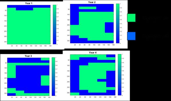
28. Deutsche Arbeitsbesprechung über Fragen der Unkrautbiologie und -bekämpfung, 27.02. – 01.03.2018 in Braunschweig

The parameter d denotes the dose, b determines the steepness of the curve an and e i is the ED 50
value of biotype i, i.e. Su(e i )=0.5.

Population dynamic and genetic model
The model is derived from the life cycle graph of an annual plant (cf. Fig. 10) with the stages seed
(S), seedlings (K), young plants (K) and adult plants (R). The transitions between the stages are
mediated by the probabilities of emergence, pA, survival of seedlings, pK, survival of young plants,
pJ, survival of seeds in soil during summer, pS and during winter, pw. The seed bank is restocked
by the number of seeds (A) produced per adult plant. For each biotype a model is set up differing
with respect to the survival probabilities under herbicide treatment. The biotypes are linked by a
genetic submodel. This conceptual model is transferred to the following time discrete equations.
Note that the model comprises 2 density dependent processes: seedling survival (eq. 14) and seed
production (eq. 16). This is important to ensure that the population is bounded. At the beginning
of a cycle K seedlings germinate from the seed bank (eq. 12). The index i denotes the biotype
K i = p A Si
           (13)
The survival of the seedlings is density dependent. The number of seedlings which can develop to
juvenile plants is limited by D max .
        Dmax K K i
 Ji =
        K+L K
           (14)
The development to mature plants depends on the survival probability Su i (d) under herbicide
dose d, which is given by a dose response function with biotype specific parameters.
Ri = J i Su i (d )
           (15)

Seed production (A) is determined by the density of adult plants R and by competition by the crop
(F).
            Amax i Rtotal
Ai =                      gi ( R)
        (1 + ε R + ϕ F )λ
           (16)
where the portion of seeds of biotype, g i (R), is given by equation (8). Finally, at the beginning of
the next cycle the seedbank (S) is updated taking into account the dormant seed of the previous
period, the surviving seed produced by mature plants in the previous period and the gain or loss
by immigration (I) from and migration (E) to adjacent plots. The indices t, i, s, w denote time,
biotype, summer and winter respectively.

S (t +1) i = ( S t i (1 − p A ) p s + Ai t ) p w + I i − Ei   i = 1,..., m
           (17)

Cellular automaton model
The local population dynamic model is embedded into a cellular automaton approach. The area
under study has the size of 180x360 m and is partitioned into rectangular grid cells of size 1x1 m.
For the simulation of precision spraying the field is portioned into subareas of size 25x36 m.
According to the weed density in a subarea, spraying is turned on or off. On each cell, the
population dynamic processes take place. Between cells, an exchange of seeds is mediated by a
bivariate Gaussian distribution. The range of seed exchange is determined by this distribution and

392                                                                                      Julius-Kühn-Archiv, 458, 2018
28. Deutsche Arbeitsbesprechung über Fragen der Unkrautbiologie und -bekämpfung, 27.02. – 01.03.2018 in Braunschweig in addition by the Moore radius. Layers of soil properties such as the pH-value or sand content influence basic parameters of the population dynamic model. Details are given in the paper of SANDT et al. (2008). Fig. 1 Basic model structure: a population dynamic- and genetic model is embedded into a cellular automaton. The gray scale symbolizes soil properties such as pH value or sand content. Abb. 1 Modellstruktur: ein populationsdynamisches -und genetisches Modell ist in einen zellulären Automaten eingebettet. Die graue Skala symbolisiert Bodeneigenschaften wie pH Werte oder Sandgehalte. Model input The dynamic behaviour of the model is determined by plant specific parameters such as D max , A max and resistance factors, environmental parameters such as soil properties, emergence probabilities of the seed (plant specific but dependent on climatic conditions), dispersion parameters such as the Moore radius and management parameters comprising application rates, weed density threshold for spraying, size of the subareas and crop rotation. In addition, the initial distribution of the seedbank in relation to biotypes is essential. General answers to the question posed in the headline therefore must be backed up by a large number of simulations with parameters out of a feasible parameter space. It should be kept in mind that the following results obtained by this model are only examples however interesting but cannot at this stage be generalized. Results and discussion The following examples refer to weeds exhibiting metabolic resistance which is assumed to be coded at three loci, giving rise to n=27 biotypes. Resistance factors were obtained as described above (eq. 11). Weed parameters were taken from the paper of SANDT et al. (2008). The cellular automaton generates spray maps based on the actual weed density in a subarea. Figure 2 shows an example. Julius-Kühn-Archiv, 458, 2018 393
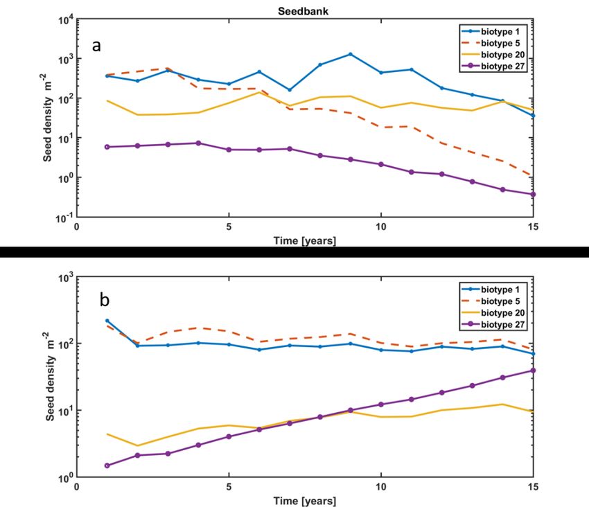
28. Deutsche Arbeitsbesprechung über Fragen der Unkrautbiologie und -bekämpfung, 27.02. – 01.03.2018 in Braunschweig

Fig. 2 Herbicide Spray maps generated by the model.
Abb. 2 Durch das Modell erzeugte Herbizid-Applikationskarten.

The next figure shows what might happen, if the management scheme favours the emergence of
resistant biotypes. In this example, there was no crop rotation and weed density threshold was
high and application rate low.

Fig. 3 Example for mismanagement. The number of plots with densities above threshold (in yellow) increases.
Abb. 3 Beispiel für missglücktes Management. Die Anzahl der Parzellen mit Unkrautdichten über dem
Schwellenwert nimmt mit der Zeit zu.

Weed density thresholds in combination with application rates have an important influence of the
emergence of resistant biotypes. Figure 4 shows the development in time of the seedbanks of
biotypes 1,5,12 and 27 for a high (Fig. 4a) and for a low threshold (Fig. 4b). The biotypes presented
are ordered with respect to their resistance factors. Biotype 1 has the lowest, biotype 27 the
highest resistance factor. These simulations were run with 40% of the possible application rates.
Low thresholds favour the emergence of resistant biotype 27. In the case of a low threshold
(10 plants/m2) the development of resistance biotypes immediately sets in. At high threshold

394                                                                                      Julius-Kühn-Archiv, 458, 2018
28. Deutsche Arbeitsbesprechung über Fragen der Unkrautbiologie und -bekämpfung, 27.02. – 01.03.2018 in Braunschweig
(50 plants/m2) the development of resistant biotypes is suppressed albeit at a cost of a high
seedbank of sensitive biotypes.
Fig. 4 Influence of weed control thresholds on the emergence of resistance. Fig 4a: 50 plant /m2, Fig 4b: 15
plants/m2. Biotype 1 has the lowest; biotype 27 has the highest resistance factor. Note that the plot is
semilogarithmic.
Abb. 4 Einfluss der Bekämpfungsschwelle auf das Aufkommen resistenter Biotypen. Fig. 4a: Bekämpfungsschwelle
50 Pflanzen /m2, Fig. 4b: 15 Pflanzen/m2. Biotyp 1 hat den niedrigsten, Biotyp 27 den höchsten Resistenzfaktor. Man
beachte die semilogarithmische Darstellung.
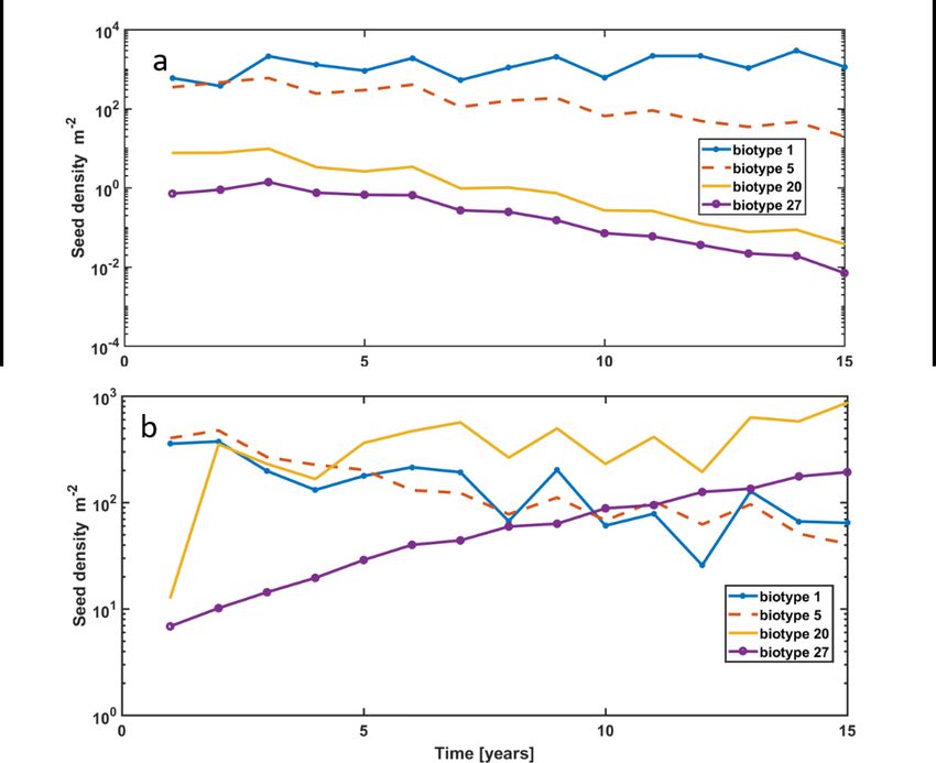
Figure 5 demonstrates the influence of the application rate on the dynamics of resistance. If the
application rate is high (Fig. 5a), under high thresholds (here 50 plants/m2) no outbreaks of
resistance occurs. Under low doses (here 40% of the maximum feasible dose) the seedbank of
resistant biotypes is increasing from the beginning (Fig. 5b).
The simulation examples support (tentatively) the formulation of the following hypotheses:
i) Weed control by precision spray technology favours the emergence of resistance at low
application rates.
ii) At high application rates even high control thresholds are tolerable.
These findings are only preliminary and have to be substantiated by exploration of the model
behaviour in the feasible parameter space together with the exploration of a large body of field
data.
Julius-Kühn-Archiv, 458, 2018 39528. Deutsche Arbeitsbesprechung über Fragen der Unkrautbiologie und -bekämpfung, 27.02. – 01.03.2018 in Braunschweig
Fig. 5 Influence of application rates on the emergence of resistance. Fig 5a: threshold 50 plant /m2and
maximum application rate, Fig 5b: threshold 50 plants/m2 and 50% of maximum application rate. Biotype 1 has
the lowest; biotype 27 has the highest resistance factor. Note that the plot is semilogarithmic.
Abb. 5 Einfluss der Aufwandmenge auf das Aufkommen resistenter Biotypen. Fig 5a: Bekämpfungsschwelle 50
Pflanze /m2 und maximale Aufwandmenge. Fig 5b: Bekämpfungsschwelle 50 Pflanzen/m2 und 40% der maximal
möglichen Aufwandmenge. Biotyp 1 hat den niedrigsten, Biotyp 27 den höchsten Resistenzfaktor. Man beachte die
semilogarithmische Darstellung.
References
BECKIE, H. J., 2006: Herbicide-Resistant Weeds: Management Tactics and Practices. Weed Technology 20, 793-814.
BUSI, R., P. NEVE and S. POWLES, 2013: Evolved polygenic herbicide resistance in Lolium rigidum by low-dose herbicide selection
within standing genetic variation. Evol Appl 6(2), 231-242.
LANGEMANN, D., O. RICHTER and A. VOLLRATH, 2012: Multi-gene-loci inheritance in resistance modling. Mathematical Biosciences
242, 17-24.
POWLES, S.B. and Q. YU, 2010: Evolution in Action: Plants Resistant to Herbicides. Annu. Rev. Plant Biol 61, 317-47.
RENTON, M., A.A.DIGGLE, I.S. MANALI and S. POWLES, 2011: Does cutting herbicide threaten the sustainablity of weed management
in cropping systems? Journal of Theoretical Biology 283, 14-27.
RICHTER, O., D. LANGEMANN and R. BEFFA (2016): Genetics of metabolic resistance. Mathematical Biosciences 279, 71-82.
SANDT, N., O. RICHTER and H. NORDMEYER, 2008: Ein raum-zeitliches Modell zur Simulation der Populationsdynamik von Unkräutern
in Hinblick auf ihre Anwendung für umweltschonender Bekämpfungsstrategien. Journal of Plant Diseases and Protection,
Special Isssue XXI, 203-208.
YU, Q., H. HAN, G.R. CAWTHRAY, S.F. WANG and S.B. POWLES, 2013: Enhanced rates of herbicide metabolism in low herbicide-dose
selected resistant Lolium rigidum. Plant Cell Environ. 36(4), 818-827.
396 Julius-Kühn-Archiv, 458, 2018You can also read