QUALITY ASSESSMENTS OF STANDARD VIDEO COMPRESSION TECHNIQUES APPLIED TO HYPERSPECTRAL DATA CUBES - IEEE-whispers

QUALITY ASSESSMENTS OF STANDARD VIDEO COMPRESSION
 TECHNIQUES APPLIED TO HYPERSPECTRAL DATA CUBES
 A.E. Oudijk1,2, F. Sigernes1,3, H.C.J. Mulders2, S. Bakken3,4, T.A. Johansen3,4
 1
 University Centre in Svalbard (UNIS), Longyearbyen, Norway
 2
 Eindhoven University of Technology (TU/e), The Netherlands
 3
 Norwegian University of Science and Technology (NTNU), Trondheim, Norway
 4
 Center for Autonomous Marine Operations and Systems (AMOS), Norway

 ABSTRACT 1.1. Hyperspectral Imaging
With a satellite-borne low-cost Hyper Spectral Imager (HSI)
a large - target area can be imaged. HSIs can detect oceanic A digital color camera uses only three values to represent
phenomena e.g. algal distribution and environmental spills, color of a pixel. The HSI gives a densely sampled, optical
enabling quicker reactions by authorities. The HSI provides spectrum for each pixel in an image. Therefore, for every
spatially resolved spectral information. The resultant datasets pixel, a spectrum on the spectral axis is stored. This produces
are large, and the capacity to transmit data to the ground is large 3D data cubes. The characteristic spectrum of an object
severely limited. To reduce the size of the dataset, can be used to classify and identify the object.
compression is required. Various freely available
compression algorithms exist. In this paper, algorithms are 1.2. Compression
assessed for their suitability for this application.
Uncompressed reference datasets from the HSI are For small satellite applications the HSI V6 (version 6) is
compressed with the H.263, H.264, and H.265 algorithms, developed [1]. The HSI V6 is a low-cost push broom imager,
varying the Quantization Parameter (QP). The compressed based on Commercial Off-The-Shelf (COTS) components.
datasets are compared to the original data using several tests. Low-cost HSIs are sensitive to experience optical distortions.
H.263 and H.264 perform the spectral tests poorly, but H.265 Therefore, wavelength and radiometric calibration are a
(QP=30) passes the spectral tests. Moreover, H.265 achieves necessity [2]. For wavelength and radiometric calibration
the best balance between quality and data reduction and is different quality parameters, for example, spectral position,
recommended for the satellite-borne HSI. intensity, and bandpass play an important role. This article
 addresses the compression effects on the quality of the data.
Index Terms— Compression Techniques, Data Cube, We would like to use existing methods of
Hyperspectral Imager, Push Broom Imaging compressing data without unacceptable spectral and spatial
 losses. In this article, the effects of various freely available
 1. INTRODUCTION lossy algorithms are investigated: the H.263, H.264, and
 H.265, originally developed for compression of video files
Hyperspectral imaging generates large amounts of data. For starting in 1990 [3]. Since then, significant improvements in
an HSI on a small satellite this is a problem because the compression are made for the H.265 algorithm [4].
amount of data that can be transmitted to earth is constrained. Another, commonly used compression method in
An S-band radio that allows only 1 Mb/s for a duration of 15 HSI is JPEG2000 [5, 6, and 7] . The JPEG2000 compression
minutes every 90 minutes, can be a typical configuration. method is compared to JP3D, which is commonly used in 3D
 To solve this problem, lossy compression techniques are medical imagery [5]. It is found that for lossy compression
considered. Lossy compression always leads to loss of JPEG2000 is outperforming JP3D [5].
information. However, lossy compression achieves higher It is found that for Principal Component Analysis
compression ratios than lossless compression. In this article, (PCA) based JPEG2000, the Signal to Noise Ratio (SNR) is
we investigate which lossy compression algorithm, originally improved [6]. The SNR improves even more if, after
developed for video compression, produces the best balance decorrelating the image using vector quantization and PCA,
between data reduction and information preservation. JPEG2000 is applied to the Principal Components. This way
 the spatial correlations for compression are optimally used.
Norwegian Research Council through the Centre of Autonomous
 To our knowledge, this new method is not compared yet to
Marine Operations and Systems (NTNU AMOS) (grant no.
223254), and the MASSIVE project (grant no. 270959). H.265 compression. However, for H.265 it is found that the
 .

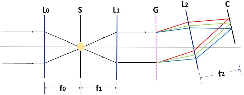
Peak Signal to Noise Ratio (PSNR) shows a better result than
JPEG2000 if both methods are used without using PCA
preprocessing [8]. Furthermore, it is found that the H.264
compression is a suitable compression for hyperspectral data
cubes [9]. Therefore, H.265 and H.264 are interesting ‘off-
the-shelf’ candidates for hyperspectral data cube
compression.
 H.265, H.264, and H.263 make use of motion
compression. For this motion compression, the algorithms
 Fig. 1: The optical diagram of the HSI V6 consisting of a
classify each (video-) frame to a certain frame type. The
 focusing front lens (L0), an entrance slit (S), a collimator
reference frames that include the most details are the intra
 (L1), a 300 grooves/mm transmission grating (G), a detector
coded (I) frames. The compression of predictive (P) and
 lens (L2), and a sensor (C).
bidirectional (B) frames benefits from this form of
compression, resulting in fewer data to represent such a
frame. The working principle of this motion compression is 2.2. Calibration of HSI V6
explained extensively in e.g. [4].
 The diffracted wavelengths are focused onto the detector
 The quality of the compression is tested using three
 array. The detector array consists of elements numbered 0 to
benchmark tests. First, a fluorescent tube reference dataset is
 1919, along the spectral dimension of the array. The
compared to a compressed dataset (E1). In this experiment,
 wavelength calibration is performed to convert this vector of
the average compression effects in intensity are compared.
 elements into a wavelength vector in units of nm [2]. Second,
Second, the hydrogen spectrum reference dataset is compared
 radiometric calibration is performed to convert counts to
to a compressed dataset (E2). Where the spectral position,
 spectral radiance. Both calibration methods are applied as for
intensity, and bandpass of the Hydrogen Alpha (Hα) peak are
 the HSI V4 in [2]. Lastly, second-order diffraction effects
investigated. Third, the wavelength calibrations performed
 occur in the HSI V6 as described by [10]. A compensation for
for measurements of the Longyearbyen Harbor as a target are
 these effects is applied to the measurements performed with
investigated (E3). The I, P and B-frames are compared in E2
 the HSI V6 before generating the final images [10].
and E3 to test the hypothesis that using a more detailed frame
type for calibration improves the calibration. For E1, E2 and
 2.3. Compression of Uncompressed Data Cubes
E3 also the Peak Signal to Noise Ratio and Cross Correlation
methods are used. Finally, a visual comparison of images of The settings of the HSI V6 during the experiments performed
the Longyearbyen Harbor is given. for this paper are given in table 1. The reference datasets used
 in this report are uncompressed (Y800) encoded. The
 2. METHODS uncompressed datasets are compressed with the software
 ffmpeg [11].
2.1. Experimental Set-up
 Table 1: Settings HSI V6.
Light rays that enter the HSI V6, see Fig. 1, are focused by
 Parameter Setting
the front lens (L0), after which the entrance slit (S) is reached.
 Compression Uncompressed (Y800)
The entrance slit has a slit height of 7 mm and a width of 50
µm. The collimator (L1) forms a parallel beam that reaches Exposure 0.03 s
the 300 grooves/mm transmission grating (G). The FPS 30
transmission grating diffracts the rays. Lastly, the light rays Gain 0 dB
are focused by the camera lens (L2) to the sensor. The lenses An important parameter in compression is the
(L0, L1, and L2) all have a focal length (f0, f1, and f2) of 50 Quantization Parameter (QP). The QP controls the amount of
mm. The sensor used is the DMK 33UX174 camera head by compression and scales from 0 to 52. A larger QP value gives
The Imaging Source Europe GmbH. The blazed transmission a higher compression. For H.263 the Qscale parameter is used
grating is optimized to measure wavelengths in the spectrum which is similar to QP, however, it scales from 0 to 31. In
of 400-900 nm [1]. The entrance slit height is too high for the these experiments the following settings are tested: H.263
detector used. Therefore, a compensation of 31 pixels in top with a Qscale of 13 and 19, H.264 with a QP of 20 and 30,
and bottom of the spectral height is performed before data and H.265 with a QP of 20 and 30. Similar QP values are used
processing. for H.264, for which it is found that these values are suitable
 for compression in [9].
 The compressions are performed on a laptop (Intel
 i7-4700MQ, 2.40GHz). The compression requires about 25
 ms per frame. For each compression a Compression Ratio

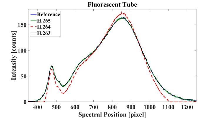
(CR) is determined. For each compressed frame it is
determined if it is classified as an I, P, or B-frame. The
uncompressed frames are all classified as I-frames.

Table 2: The CR for E1, E2, and E3 for each compression
algorithm.
 Compression CR E1 CR E2 CR E3
 H.265 QP 30 1.43E+04 1.46E+05 3.73E+05
 H.265 QP 20 1.17E+02 1.55E+04 1.07E+03
 H.264 QP 30 1.87E+04 1.46E+05 2.46E+03
 H.264 QP 20 6.52E+01 1.55E+04 6.32E+02
 H.263 Qscale 19 5.03E+02 7.03E+02 4.25E+02 Fig. 2: Intensity for each spectral position averaged over 148
 H.263 Qscale 13 4.75E+02 7.22E+02 3.89E+02 frames.
 dimension of the array, for E3, can be seen in Fig. 7. For
2.4. Metric Methods H.264 a large variance can be seen for all experiments, which
 is probably caused by intensity distortion.
The Cross Correlation (CC) and Peak Signal to Noise Ratio
(PSNR) are determined by (1) and (2), respectively. Where σ 3.2. Fluorescent Tube Spectrum Experiment (E1)
is the standard deviation, and tar and ref are the intensity for
each spectral position for the compressed and reference Fig. 2 shows the intensity centerlines of the datasets for all
datasets, respectively. In the Mean Squared Error (MSE), the QP and Qscale values. The reference, H.265, and H.263
intensity for each spectral position for the compressed dataset datasets are given in blue, green and black, respectively.
is compared to this value of the reference dataset. The CC and These datasets are overlapping. The H.264 datasets are given
PSNR are evaluated over all frames, and over the full, in red. From this figure, it is observed that the intensity of the
compensated, slit height. H.264 compression is distorted. This distortion results in an
 average PSNR for H.264 that is 10 dB lower than for H.265
 ( , ) and H.263, see table 3.
 = (1)
 
 = 20 log10 (
 255
 ) (2) 3.3. Hydrogen Experiment (E2)
 √ 
 The average spectral position, intensity, and bandpass in a Hα-
 3. RESULTS peak for each I, P and B-frame are shown in Fig. 3. For
 clarity, the reference dataset is added to each frame-type row.
3.1. Compression Ratio The dotted line shows the standard deviation of the reference
 datapoints. Between the different frame-types, there is not a
The average CR for the datasets of E1 (148 frames), E2 (1010 significant difference observed. The spectral position is
frames), and E3 (5335 frames) is given in table 2. In table 2 determined with a maximum difference of 1 pixel for all
it can be seen that for a QP of 20 and 30 the CR of H.265 and compression methods. Deviations can be observed for
H.264 are similar. One exception is found for E3, where intensity and bandpass.
H.265 achieves the highest CR. The CR of H.263 is the lowest All three quality criteria are reconstructed outside
for all experiments. the 95% interval of the reference dataset after H.263
 The CC and PSNR, averaged over the slit width, for compression. This results in a CC and PSNR higher than for
each experiment are given in table 3. In E2 the intensity H.264 and lower than for H.265, as can be seen in table 3.
differs for the Hα-peak from 200 counts to 0 counts in only 20 The intensity and bandpass show a smaller deviation from the
pixels. In E3, due to the outside scenery there is also a large reference point when a smaller Qscale is used. After H.264
variety in intensity. This is causing a large variance of the compression both QPs give similar results.
PSNR for E2 and E3. The PSNR over the full spectral

 Table 3: The CC and PSNR of H.265, H.264, and H.263 with the reference dataset.
 Compression CC E1 CC E2 CC E3 PSNR (dB) E1 PSNR (dB) E2 PSNR (dB) E3
 H.265 QP 30 0.97 ± 0.00 0.87 ± 0.06 0.99 ± 0.00 32 ± 6 30 ± 101 37 ± 25
 H.265 QP 20 0.97 ± 0.00 0.91 ± 0.03 0.99 ± 0.00 32 ± 8 31 ± 91 39 ± 30
 H.264 QP 30 0.97 ± 0.00 0.69 ± 0.20 0.82 ± 0.08 21 ± 85 15 ± 153 18 ± 148
 H.264 QP 20 0.97 ± 0.00 0.69 ± 0.20 0.82 ± 0.08 23 ± 84 15 ± 175 18 ± 153
 H.263 Qscale 19 0.96 ± 0.00 0.81 ± 0.11 0.98 ± 0.00 31 ± 9 22 ± 93 33 ± 19
 H.263 Qscale 13 0.96 ± 0.00 0.82 ± 0.12 0.99 ± 0.00 31 ± 8 23 ± 97 34 ± 20

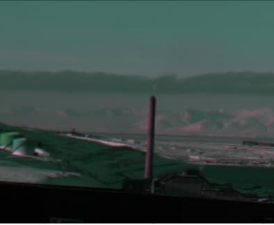
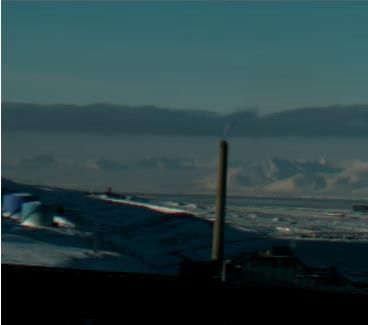
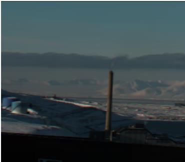
Fig. 5: A reference uncompressed
 RGB-image (MNC 122), obtained
Fig. 3: Average spectral position, intensity and bandpass for Hα, with the with the HSI V6.
corresponding standard deviation. The bandpass is determined with [12]. The
standard deviation of the reference data points is shown within the dotted
lines.
Furthermore, an intensity distortion can be observed, similar difference for all frame-types and both QP values. After the
as shown in Fig. 2. The bandpass appears sharper than the wavelength calibration, the Fraunhofer peaks are found
bandpass of the reference dataset. These distortions result in within 0.7 nm from the reference dataset, again for all frame-
the lowest CC and PSNR for H.264 for E2 as can be seen in types and both QP values of H.265. Therefore, the
table 3. For H.265 compression both QPs give similar results. wavelength calibration is unaffected for a specific frame-
It is found that the H.265 performs best for all three quality type or QP 30 or 20.
criteria. Moreover, H.265 shows the highest CC and PSNR in
table 3 for E2, however the variance found in PSNR is high. 3.5. Longyearbyen Harbor Images (E3b)

3.4. Wavelength calibration for Longyearbyen Harbor The reference RGB-image obtained of the Longyearbyen
 images. (E3a) harbor can be seen in Fig. 5. The image is constructed by
 using the calibrations described in section 2.2. The intensities
After H.263 compression, details in the spectrum are lost. in all images are normalized to the Maximum Number of
Therefore, it is not possible to determine the Fraunhofer peaks Counts (MNC), found in each image, see image descriptions.
in the spectrum. This makes wavelength calibration after The wavelengths used for constructing the images are 680 nm
H.263 compression impossible. For H.264 and H.265 for red, 540 nm for green, and 480 nm for blue. A spectral
detection of the Fraunhofer peaks is possible. In Fig. 2 and 3 bandpass of 3.5 nm is applied.
it is already shown that H.265 performs best for all quality The H.265 and H.264 RGB-images are obtained
criteria. Therefore, it is interesting to optimize the use of similarly, (mutatis mutandis), see left of Fig. 4 and 6. It is
H.265. The spectral position of the Fraunhofer peaks of the difficult to notice the differences by eye. Therefore, the
reference and H.265 dataset is compared. This is done for the compressed dataset is subtracted from the reference dataset.
different frame-types and a QP of 30 and 20. It is found that The results can be seen in the right images in Fig. 4 and 6. It
the Fraunhofer peaks are detected with at most 2 pixels can be observed that the contours of the image are visible for
 green and blue for H.265 compression. The contours of the
 subtracted image are more clearly visible for the H.264
 compression, where also red can be distinguished. These
 observations are supported by the CC of both compression
 methods, see table 3. The CC of H.265 is higher than the CC
 of H.264. Furthermore, the PSNR is overall higher for H.265.
 The distorted PSNR-peaks in Fig. 7 are located at the
 Fraunhofer peaks B and A. At these peaks, a small amount of
 counts is detected, causing the distortion in the PSNR.

Fig. 4: Compressed H.265 QP30 RGB-image (MNC 121)
(L) and the compressed image subtracted from the
reference image (MNC 83) (R).

5. REFERENCES

 [1] Sigernes, F. (2018). Pushbroom hyper spectral imager
 version 6 (HSI V6) part list - final prototype. Unpublished.

 [2] Henriksen, M. B., Garrett, J. L., Prentice, E. F., Stahl,
 A., Johansen, T. A., & Sigernes, F. (2019, September). Real-
 Time Corrections for a Low-Cost Hyperspectral Instrument.
 In 2019 10th Workshop on Hyperspectral Imaging and
 Signal Processing: Evolution in Remote Sensing
Fig. 6: Compressed H.264 QP30 RGB-image (MNC 138)
 (WHISPERS) (pp. 1-5). IEEE.
(L) and the compressed image subtracted from the reference
image (MNC 89) (R).
 [3] Liou, M. (1991). Overview of the p× 64 kbit/s video
 coding standard. Communications of the ACM, 34(4), 59-63.

 [4] Sayood, K. (2012). Introduction to data compression.
 Newnes.

 [5] Zhang, J., Fowler, J. E., Younan, N. H., & Liu, G. (2009,
 July). Evaluation of JP3D for lossy and lossless compression
 of hyperspectral imagery. In 2009 IEEE International
 Geoscience and Remote Sensing Symposium (Vol. 4, pp. IV-
 474). IEEE.

 [6] Du, Q., & Fowler, J. E. (2007). Hyperspectral image
 compression using JPEG2000 and principal component
 analysis. IEEE Geoscience and Remote sensing letters, 4(2),
 201-205.
Fig. 7: PSNR for E3 with Fraunhofer lines
 [7] Báscones, D., González, C., & Mozos, D. (2018).
 Hyperspectral image compression using vector quantization,
 4. CONCLUSION PCA and JPEG2000. Remote Sensing, 10(6), 907.
H.265 compression reproduces the spectral position,
intensity, and bandpass closest to the reference dataset. From [8] Pestel-Schiller, U., Vogt, K., Ostermann, J., & Groß, W.
Fig. 3 it can be seen that H.265 compresses the intensity (2016, December). Impact of hyperspectral image coding on
correctly, whereas H.263 and H.264 show a distortion. The subpixel detection. In 2016 Picture Coding Symposium
distortion of H.264 is also found in the PSNR, which is on (PCS) (pp. 1-5). IEEE.
average 15 dB lower than the PSNR of H.265. However, the
PSNR shows a high variance, especially for the H.264 [9] Santos, L., Lopez, S., Callico, G. M., Lopez, J. F., &
compression. The CC of H.265 is, on average, 21% higher Sarmiento, R. (2011). Performance evaluation of the H.
than the CC of H.264. The differences between the reference 264/AVC video coding standard for lossy hyperspectral
and the H.265 and H.264 (QP=30) are also visualized in Fig. image compression. IEEE Journal of Selected Topics in
4 and 6. It can be seen that the H.265 compression shows Applied Earth Observations and Remote Sensing, 5(2), 451-
great similarity with the reference image. Furthermore, it is 461.
discussed that for H.265 the wavelength calibration is
unaffected for a specific frame-type or QP 30 or 20. Finally, [10] Van Hazendonk, L. (2019). Calibration of a hyper
from table 2 it can be seen that the average CR of the H.265 spectral imager. Master Internship Report. Unpublished.
with a QP of 30 is the highest. Therefore, it is recommended
to use H.265 with a QP of 30 for compression of [11] FFmpeg Developers. (2016). ffmpeg tool (Version
hyperspectral data cubes. be1d324) [Software]. Available from http://ffmpeg.org/.

 [12] Egan, P. (2020). fwhm
 (https://www.mathworks.com/matlabcentral/fileexchange/10
 590-fwhm). MATLAB Central File Exchange. Retrieved
 October 14, 2020.