Donut as I do: Learning from failed demonstrations
←
→
Page content transcription
If your browser does not render page correctly, please read the page content below
Donut as I do: Learning from failed demonstrations
                                        Daniel H Grollman and Aude Billard
                                 Learning Algorithms and Systems Laboratory, EPFL
                                {daniel.grollman, aude.billard}@epfl.ch

   Abstract— The canonical Robot Learning from Demonstra-
tion scenario has a robot observing human demonstrations of
a task or behavior in a few situations, and then developing a
generalized controller. Current work further refines the learned
system, often to perform the task better than the human could.
However, the underlying assumption is that the demonstrations
are successful, and are appropriate to reproduce. We, instead,
consider the possibility that the human has failed in their
attempt, and their demonstration is an example of what not
to do. Thus, instead of maximizing the similarity of generated
behaviors to those of the demonstrators, we examine two meth-
ods that deliberately avoid repeating the human’s mistakes.

                     I. I NTRODUCTION
   One current problem in robotics is that while modern
robots are physically capable of performing many useful
tasks (e.g. heart surgery, space-station repair, bomb disposal),
they are only able to do so under constant supervision and
control of expert human operators or in highly engineered
environments. That is, what are lacking are autonomous             Fig. 1: An overview of our approach. After modeling col-
controllers for performing these skills in novel situations        lected failed demonstrations as in regular RLfD, we generate
without human oversight. Robot Learning from Demonstra-            exploratory trajectories by assuming that when demonstra-
tion (RLfD) is an attempt to fill this void by enabling new        tions disagree, they actually indicate what not to do. We
robot controllers to be developed without requiring analytical     update the model after exploration and repeat until successful
deconstruction and explicit coding of the desired behavior.        task performance or trajectory convergence. In all figures
   Currently, RLfD typically first collects a set of exam-         distributions are shown ± 3 standard deviations.
ples, wherein a human user demonstrates acceptable task
execution. These examples are then somehow put into the
robot’s frame of reference, and a generalized control policy is                        II. R ELATED W ORK
extracted. This policy can be improved via further interaction        Of course, a human’s failed demonstrations are not entirely
with the human, or by optimizing known or inferred criteria.       devoid of useful information. We assume that the humans are
   Many different approaches along these lines exist [1],          attempting to perform the desired task, and not performing
[2], and as the field coalesces, overarching formalisms are        unrelated motions. Failure is then due perhaps to lack of
being developed [3]. We note that early work was typically         skill or effort. We draw inspiration from work with humans
in discrete state and action spaces and took the human             showing that infants are able to successfully perform tasks
demonstrations as indicative of correct or optimal behav-          that they have only seen failed examples of [4].
ior. However, as recent research has shifted to continuous            In RLfD, the most closely related work assumes the
domains, there is more focus on optimizing the learned             demonstrations are correct, yet suboptimal, and incorpo-
behavior beyond the demonstrator’s capabilities.                   rates Reinforcement Learning (RL) to optimize the learned
   In this paper, we propose to take the next logical step.        system. For example, the PoWER algorithm uses demon-
That is, the initial assumption (which was valid in small,         strations to initialize a policy, and then improves it with
finite, discrete spaces) was that human demonstrations were        respect to a known reward function by performing ex-
optimal and the robot was told to “Do as I do.” Currently,         ploratory rollouts, perturbing the the current policy by state-
this assumption is being relaxed to allow improvement over         dependent noise [5]. One drawback is that if the initial
the demonstrations, which still positively bias the robot:         demonstrations are very suboptimal (such as failures), this
“Do nearly as I do.” We here consider the situation where          and similar techniques may be unable to locate a successful
the humans are not only sub-optimal, but incapable of              policy. By acknowledging the failure of demonstrations and
performing the task, and their demonstrations must be treated      deliberately avoiding them, we here provide an alternate
in part as negative biases: “Do not as I do.”                      means of generating exploratory trajectories.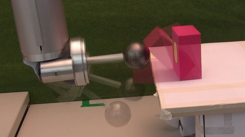
Alternatively, if the reward function is not known, or the       maximize the probability of observed data for a given
user does not wish to specify one, Inverse Reinforcement            value of K, and the Bayesian Information Criterion [13],
Learning (IRL) techniques can estimate one from the demon-          a penalized likelihood method, to select K itself. As K is
strations themselves [6]. The current state-of-the-art requires     discovered in a data-driven fashion, our overall technique
that the reward function be linear in the feature space, so         can be considered nonparametric – the total number of
feature selection is very important. Further, they allow for        parameters used to model the data is not set apriori.
the inclusion of prior information, indicating which features          To compute ξ˙ for a given ξ we require the conditional:
are the most important or what their values should be. By                                   K
                                                                              ˙ θ) =                         ˙ µ̃k (ξ, θ), Σ̃k (θ)) (2)
                                                                                            X
providing ‘correct’ values for some features, the system is                P (ξ|ξ,              ρ̃k (ξ, θ)N (ξ;
told, in effect, to ignore certain aspects of the demonstrations.                           k=1
We note here that ignoring portions of the demonstrations is                k
                                                                           µ̃ (ξ, θ) =      µkξ̇ +
                                                                                                            −1
                                                                                                     Σkξ̇ξ Σξξ
                                                                                                            k
                                                                                                               (ξ − µkξ )                  (3)
not the same as actively avoiding them.                                                                       −1
   The above techniques learn an initial model from demon-                   Σ̃k (θ) = Σkξ̇ξ̇ − Σkξ̇ξ Σkξξ Σkξξ̇                           (4)
stration, and improve it on their own. Alternate work contin-                                ρ   k
                                                                                                     N (ξ; µkξ , Σkξξ )
ues to use the demonstrator during the learning process, to                ρ̃k (ξ, θ) =     PK                                             (5)
provide more information. For example, corrective demon-                                       k=1    ρk N (ξ; µkξ , Σkξξ )
strations may be provided when the learned policy acts              Note that Σ̃k does not depend on the current state. For clarity
inappropriately [7], [8]. However, these techniques assume          we drop the functional forms of the conditional parameters.
that the demonstrator is able to perform what should have             This conditional distribution over ξ˙ is itself a GMM, with
been done, and that either the training was ambiguous, or           an overall mean and variance:
the learning was incorrect. Instead users may simply indicate                                             K
how the behavior should change using a set of operators, and                                 ˙ θ] =
                                                                                                          X
                                                                                          Ẽ[ξ|ξ,               ρ̃k µ̃k                    (6)
therefore train a system that outperforms themselves, without
                                                                                                          k=1
needing to explicitly specify a reward function [9].
                                                                                                                 K
   These approaches all assume that the initial demonstra-               ˙ θ] = −Ẽ[ξ|ξ,
                                                                                    ˙ θ]Ẽ[ξ|ξ,
                                                                                           ˙ θ]⊤ +
                                                                                                                 X
                                                                     Ṽ [ξ|ξ,                                          ρ̃k (µ̃k µ̃k⊤ +Σ̃k ) (7)
tions are basically correct, and that issues remaining after
                                                                                                                 k=1
learning are due to stochastic humans or improper learning
(poor generalization, simplified models, etc). Fully failed           As   illustrated in Figure 1, our general approach is to:
demonstrations are usually discarded, either explicitly by            1)   Collect a set of failed demonstrations (X).
researchers, or implicitly in the algorithms themselves. We           2)   Build a model of what the demonstrators did (θ).
believe that these failures have instructive utility and can          3)   Use the model to generate a tentative trajectory that
place constraints on what should and should not be explored.               explores near the demonstrations (x∗ ).
                                                                        4) Run x∗ , update θ.
                    III. M ETHODOLOGY                                   5) Repeat steps 3-4 until success or convergence.
   We compare approaches to RLfD of motion control based                Step 3 is the key, where we generate full trajectories from
on Dynamical Systems (DS) [10] and Gaussian Mixture                 an initial state (ξ1∗ ) by predicting a velocity, updating the state
                                                                    with that velocity, and repeating: x∗ = {ξt∗ , ξ˙t∗ }Tt=1 , ξt+1
                                                                                                                             ∗
                                                                                                                                 ∗
Models (GMM)[11]. Taking the state of the robot, ξ and                                                                                =
                                                                      ∗    ˙∗                              ˙
                                                                    ξt + ξt . Prediction stops when ξ = 0 or a predetermined
its first derivative ξ˙ to be D-dimensional vectors, a demon-
stration is a trajectory through this state-velocity space,         time-length (1.5 times the longest demonstration) is passed.
xn = {ξtn , ξ˙tn }Tt=1 . From a set of N demonstrations X =
                    n
                                                                    With faster computation we could generate velocities online,
{x }n=1 of possibly different lengths (T i 6= T j , i 6= j), we
   n N                                                              to react to perturbations and noise in the actuators. We use
approximate the distribution of observed state-velocity pairs       a low-level high-gain PID controller to avoid these issues.
with a GMM where the probability of a given pair is:                    For step 4, there are multiple ways to update the GMM
                                                                    incrementally [12]. A naive approach is to retrain the GMM
                           K
                   ˙ =
                           X
                                          ˙ µk , Σk )               on all of the available data. However, computation grows
             P (ξ, ξ|θ)          ρk N (ξ, ξ;                 (1)    with the number of datapoints. We instead sample a fixed
                           k=1
                                                                    number of points from the current GMM, weight them to
N is the standard normal distribution and θ =                       represent the total number of data points, and then combine
{K, {ρk , µk , Σk }K
                   k=1 } are the collected parameters, termed       them with the new trajectory for re-estimation. Note that K
the number of components (positive integer) and the priors          is unchanged in this approach.
(positive real, sum to 1), means (2D real vector) and covari-           Below we describe our different techniques for predicting
ances (2D × 2D psd matrix) of each component.                       a velocity for a given state from learned models. They are
    To deal with mismatches in the size of the state and            compared graphically in Figure 2. Our main intuition is that
velocity spaces, we first normalize our data such that all          while the demonstrators are not succeeding, they are at least
dimensions are mean zero and have unit variance. We then            attempting to (roughly) perform the task. Thus, exploring
fit these parameters using a combination of the Expectation-        in the vicinity of the demonstrations, while avoiding them
Maximization algorithm [12] (initialized with Kmeans) to            exactly, may lead us to discover a way to succeed.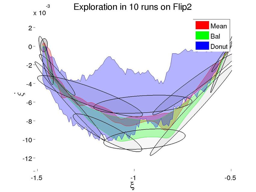
0.16                                                               0.5
                                     GMM(ξ̇|ξ, θ)                                                                                          ˙ 0, 1)
                                                                                                                                       N (ξ|ξ,
                                     DMM(ξ̇|ξ, θ)                           0.45                                                       D(ξ̇|ξ, 0, 1, ǫ)
          0.14
                                     ξ˙MEAN
                                                                                                                      ε=0
                                     ξ˙BAL                                   0.4
          0.12                       ξ˙DNT
                                     ξ˙MIN                                  0.35
           0.1                       ξ˙MAP
                                                                             0.3
P (ξ|ξ)

                                                                  P (ξ|ξ)
   ˙

          0.08

                                                                     ˙
                                                                            0.25

                                                                             0.2
          0.06
                                                                                                                            ε = 0.25
                                                                            0.15
          0.04
                                                                             0.1                                                 ε = 0.5
                                                                                                                                      ε = 0.75
          0.02                                                                                                                             ε=1
                                                                            0.05

             0                                                                 0
            −10          −5             0           5       10                −10              −5                0                 5                      10
                                        ξ˙                                                                       ξ˙

Fig. 2: Illustration of velocities generated by the different     Fig. 3: The donut pseudo-inverse has an additional explo-
techniques introduced for a particular state. The dashed          ration parameter that determines how far away the peaks are
distribution is the GMM, and the solid distribution is what       from the base distribution.
arises after replacing all Gaussians with Donuts.

                                                                  only one class (and its mean) is updated at each iteration,
A. Approach 1: Balanced Mean                                      shifting the overall mean. By assumption correct behavior
   A standard way to use GMMs in RLfD is to assume that           lies somewhere between the two classes, and this technique
the demonstrations are optimal, but corrupted by mean-zero        approaches it in a fashion similar to that of binary search.
Gaussian noise. Thus the expected value of the conditional           A further advantage of this technique is that when the
distribution (Equation 6) estimates the noise-free function:      classes ‘agree’ (produce nearly the same mean) then ξ˙BAL ≈
                                                                  ξ˙MEAN . This situation corresponds directly with assuming
                              ξ˙MEAN = Ẽ[ξ|ξ,
                                          ˙ θ]              (8)   that the demonstrations are noisily correct1 . Thus, overall,
   However, in our scenario this assumption does not hold.        this approach will follow the demonstrations when the two
Particularly, as the demonstrations are failures, we do not       classes agree and explore in between the data when the two
assume they are Gaussianly distributed around success, and        classes disagree, which follows from our intuition that the
thus do not expect their mean to succeed. Further, incorpo-       demonstrations, while failures, are not all wrong.
rating the mean of a GMM back into the model will not lead        B. Approach 2: Donut MAP
to improvement, as the mean itself becomes more likely.            An alternate technique for generating velocities from a
   As an alternative we employ a balanced mean approach,          GMM is to use the Maximum a posteriori (MAP) value:
which allows for improvement over iterations. We divide X
into two classes: X+ and X− , reasoning that demonstrators                                                       ˙ θ)
                                                                                             ξ˙MAP = argmaxξ̇ P (ξ|ξ,                               (10)
that fail do not blindly repeat themselves. Rather, they try to   Doing so makes sense when operating in non-convex spaces,
correct themselves, and may end up failing in a different         where the combination of two successful demonstrations may
fashion. A binary division is the simplest case, but the          not be appropriate. For example, turning left and turning
approach may scale to multiple classes and dimensions.            right at a cliff’s edge are both viable, but their convex mean
   From these two classes, we derive two GMMs parame-
                                                                  (walk forward) is not. Similar to the standard mean, we
terized by θ+ and θ− . Our overall estimated velocity is a
                                                                  observe that using the MAP incrementally will lead to rapid
weighted average of the means from each class:
                                                                  convergence and minimal improvement. However, with our
                  ξ˙BAL = αẼ[ξ|ξ,
                              ˙ θ+ ] + (1 − α)Ẽ[ξ|ξ,
                                                 ˙ θ− ]     (9)   assumption that demonstrations are indicative of what not to
                                                                  do, an alternate possibility is to generate those trajectories
where α ∈ [0, 1] is a mixing ratio. We set α = 0.5, but in        that are least likely under the model of the demonstrations,
the future may make α state-dependent, perhaps measuring          guaranteeing that we perform not-like the users:
the relative variance in the predictions from the two classes.
   The generated trajectory is necessarily in between the                                                         ˙ θ)
                                                                                              ξ˙MIN = argminξ̇ P (ξ|ξ,                              (11)
means of the two classes, so this approach requires that the         Two issues arise when using the minimum likelihood
demonstrations ‘span’ the area where correct behavior lies.       technique: 1) local minima only exist between the demonstra-
If the classes are balanced to begin with (same number of         tions, beyond the data the conditional probability continues
demonstrated points), then Equations 9 and 6 are the same.
However, as the generated trajectories are incorporated,              1 Another     possibility is that there is a bias in the demonstrations.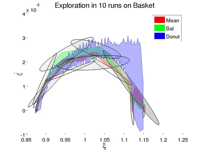
(a) FlipUp                                                           (b) Basket

Fig. 4: Our robot tasks. FlipUp: get the foam block to stand on end, Basket: Launch the ball into the basket. Shown are
successful trajectories learned with the Donut MAP approach from 2 initial failed demonstrations.

to decline. 2) local minima are always off of the data, so             joint angles (ξ) at 500Hz. Velocities ξ˙ are computed as the
even when demonstrations are in agreement we avoid them.               single-step difference between samples (ξ˙t = ξt+1 − ξt ).
   We address both issues by instead finding a maxima of                  While the tasks themselves are fairly simple (1DOF) and
a mixture of pseudo-inverses of the Gaussian distribution.             performable by human demonstrators, it often takes them a
Each individual component of the GMM (N (ξ;           ˙ µ̃k , Σ̃k ))   few tries to get it right. In standard RLfD, these failures
is replaced by its pseudo-inverse, the donut distribution              would be ignored, and only the successful performances
(D(ξ;˙ µ̃k , Σ̃k , ǫ)), resulting in a Donut Mixture Model             used. We instead learn only from these failures. We note that
(DMM). The additional exploration parameter (ǫ ∈ [0, 1])               all of our demonstrations are complete, in that task failure
allows us to generate a spectrum of distributions whose peaks          does not lead to early termination of the attempt.
smoothly move from that of the underlying base distribution               To evaluate our techniques we are concerned not only with
to a configurable maximum distance away, as seen in Figure             whether or not the task is eventually performed successfully
3. Further details about D are in the appendix.                        (which it is), but also with the breadth of possibilities that
   We use the overall variance of the conditional (Equation            are generated. That is, as continued failure is observed, we
7) to set exploration: ǫ = 1 − 1+||V [1ξ̇|θ,ξ]|| . Our reasoning       want to generate trajectories that diverge more from the
is that if the variance of the conditional is low, then the            demonstrations, exploring where no human had gone before,
multiple demonstrations are in agreement as to what velocity           while at the same time reproducing the parts of the task that
should be associated with the current state. In this situation,        the different demonstrators agree on.
it makes sense to do what the model predicts. However, if
the variance is high, the demonstrations do not agree, and it          A. Task 1: Flip Up
would therefore be sensible to try something new.                          Our first task, illustrated in Figure 4a, is to get a square
   Our actual desired velocity is the most likely velocity:            foam block to stand on end. The block is set at the edge of
                               K
                                                                       a table, with a protruding side, but not fixed to the table in
                                                                       any way. Using the robot’s wrist, the end effector comes from
            ξ˙DNT = argmaxξ̇               ˙ µ̃k , Σ̃k , ǫ)
                               X
                                     ρ̃k D(ξ;                  (12)
                                                                       below and makes contact with the exposed portion. The setup
                               k=1
                                                                       is such that the block cannot be lifted to a standing position
where each of the conditional Gaussian components has been             while in contact with the robot. Instead, there must be a
replaced by its pseudo-inverse. However, as there is no closed         ‘flight’ phase, where the block continues to move beyond
form for the optima of a GMM we use gradient ascent to                 the point in time when the robot ceases contact. Thus, the
find a local maximum in the area around an initial guess,              robot must impart momentum to the block. However, too
ξ˙′ . For a new trajectory we initialize ξ˙1′ = ξ˙1MEAN and take       much momentum and the block will topple over.
ξ˙t+1
  ′
       = ξ˙tDNT for the other timesteps.                                   We collect 2 demonstrations of this task. In the first, too
                                                                       little momentum is transferred, and the block falls back to
                 IV. E XPERIMENTAL S ETUP
                                                                       the initial position. In the second, too much momentum is
   We test the above approaches on two tasks that are difficult        imparted, and the block topples the other way. The resulting
for human demonstrators to perform. The accompanying                   initial GMM is shown in state-velocity space in Figure
video shows the tasks being demonstrated and the results of            5a. We see that both demonstrations have the same basic
learning with Donut MAP. Our robot is the Barrett WAM,                 shape, but differ in their maximum velocity and their timing.
and we collect demonstrations kinesthetically, by placing              Further, they agree on starting and ending positions of the
the used joint in gravity-compensation mode and physically             task. These agreements should be reproduced in the trial
guiding it in attempts to perform the task while recording             trajectories, while areas of disagreement are more explored.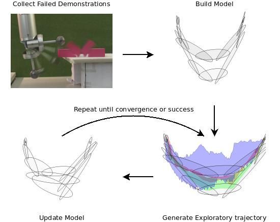
(a) FlipUp                                                         (b) Basket

      Fig. 5: Illustrations of the initial GMMs and the space of trajectories explored for each task by the techniques.

B. Task 2: Basket Ball                                              in our experiments the donut method took more iterations to
   The second task we consider also depends on accurate             succeed than the balanced mean.
velocity control. Our basketball setup, shown in Figure 4b,            Further, as expected, exploration with both techniques
has the robot launching a small ball with a catapult, with the      increased in the middle portions of both tasks, where the
goal of having the ball land in a basket attached to a wall         demonstrations disagreed the most. At the beginning (and
opposite. Our initial position has the robot’s end effector         to a lesser extent the end), the generated trajectories more
already touching the catapult, so all necessary force must be       closely resemble the humans’. This behavior is more visible
built up relatively quickly.                                        in Figure 5a, which has more variance. We believe the
   We again collect two demonstrations, one from each class         decreased agreement at the end of the movement comes from
in the Balance Mean approach. The first causes the ball to          accumulated drift during trajectory generation.
rebound off of the wall above the basket, and the second               What these plots do not show is the order in which
below. The initial model is in Figure 5b.                           trajectories are generated. For the BAL technique, the initial
                                                                    trajectory is at the midpoint between the two demonstra-
                       V. D ISCUSSION                               tions. Successive trajectories then approach the negative class
   As expected, the standard mean and MAP techniques                incrementally. Donut, on the other hand, is much more
rapidly converge to unsuccessful policies. While some explo-        erratic in its exploration: The technique will generate a
ration takes place (due to changes in the underlying models),       few trajectories on one side of the data (slower than all
the generated trajectories are very limited and cover a small       demonstrations), and then jump to exploring in between the
portion of the available state-velocity space. Likewise, the        demonstrations, and then jump again to being faster.
minimum technique leads to issues, generating velocities that          We believe this behavior (and some of the visual jagginess)
are not physically safe for the robot.                              arises from our use of gradient ascent in the velocity gener-
   In terms of finding a successful policy, both the Donut          ation and our initialization. Since we are only finding a local
MAP (DNT) and Balanced Mean (BAL) techniques converge               maximum, it may be that the generated velocity is actually
within 10 iterations. However, the exploration exhibited by         relatively unlikely. However, it will keep being selected until
each algorithm is distinctly different. To illustrate the breadth   the model has shifted enough to remove the local optimality.
of the search from each technique, we show the spread of 10         Further, as we initialize with the mean at t = 1, we will
generated trajectories from each algorithm for each task in         always start at the local maxima nearest to it, which may
Figure 5. For this illustration, we have assigned all generated     unnecessarily curtail our exploration.
trajectories to the same class (+). For comparison, we show
                                                                                        VI. F UTURE W ORK
the area explored by the standard mean.
   We immediately see that of the three, the donut technique           We are examining ways to alleviate these issues and im-
covers the widest area, by an order of magnitude. While both        prove Donut’s performance. One approach is to use sampling
mean-based approaches are limited to generating trajectories        in an attempt to find the global maxima instead of a local
inside the span of the demonstrations, the donut is not,            one. However, each additional sample would require its own
which will allow it to succeed if all demonstrations are            gradient ascent, which is computationally costly. Further, the
in one class (e.g, too low). However, this advantage has a          global maxima may shift greatly from one timestep to the
downside. Because there are more possibilities to explore,          next, generating potentially unsafe velocities and torques.
We have also considered introducing a forgetting factor [3] E. A. Billing and T. Hellström, “A formalism for learning from
into our GMM update. Currently, we resample only to speed demonstration,” Paladyn, vol. 1, no. 1, pp. 1–13, 2010.
[4] A. N. Meltzoff, “Understanding the intentions of others: Re-enactment
up the estimation of the updated parameters, and weigh our of intended acts by 18-month-old children,” Developmental Psychol-
samples to represent the total number of datapoints. We could ogy, vol. 31, no. 5, pp. 838–850, 1995.
instead force the old data to have the same weight as the [5] J. Kober and J. Peters, “Policy search for motor primitives in robotics,”
in Neural Information Processing Systems, Vancouver, Dec. 2008.
newly generated trajectory (or some percentage of the old [6] P. Abbeel, D. Dolgov, A. Y. Ng, and S. Thrun, “Apprenticeship learn-
weight), which may speed exploration. However, there is ing for motion planning with application to parking lot navigation,”
then the worry that the original demonstrations will be lost. in International Conference on Intelligent Robots and Systems, Nice,
France, Sept. 2008, pp. 1083–1090.
In terms of the BAL approach, we currently hand-assign [7] S. Chernova and M. Veloso, “Interactive policy learning through
trajectories to one of the two classes. For our tasks, this is confidence-based autonomy,” Journal of Artifical Intelligence Re-
an acceptable method. However, as the behaviors become search, vol. 34, no. 1, pp. 1–25, Jan. 2009.
[8] D. H. Grollman and O. C. Jenkins, “Dogged learning for robots,” in
more complex and high-dimensional, it may no longer be. International Conference on Robotics and Automation, Rome, Italy,
One possibility would be to first use unsupervised clustering Apr. 2007, pp. 2483 – 2488.
to automatically divide the data into (possibly more than [9] B. Argall, B. Browning, and M. Veloso, “Learning by demonstration
with critique from a human teacher,” in International Conference on
two) classes. Additionally, making the mixing parameter (α) Human-Robot Interaction, Arlington, VA, Mar. 2007, pp. 57–64.
dependent on the current state may enable us to explore more [10] M. Hersch, F. Guenter, S. Calinon, and A. Billard, “Dynamical system
heavily when the demonstrations disagree more, in much the modulation for robot learning via kineshetic demonstrations,” IEEE
Transactions on Robotics, pp. 1463–1467, 2008.
same way the donut does now. [11] H. G. Sung, “Gaussian mixture regression and classification,” Ph.D.
Looking at our work through the lens of reinforcement dissertation, Rice, 2004.
learning, you can think of us as currently using a binary [12] R. Neal and G. E. Hinton, “A view of the EM algorithm that justifies
incremental, sparse, and other variants,” in Learning in Graphical
reward signal: Success or failure, and we assume all of Models. Kluwer Academic Publishers, 1998, pp. 355–368.
our demonstrations fail. Rather than exploring randomly [13] X. Hu and L. Xu, “Investigation on several model selection criteria for
in the space of possible trajectories, we generate guesses determining the number of cluster,” Neural Information Processing. -
Letters and Reviews, vol. 4, no. 1, pp. 1–10, July 2004.
based on the intuition that failure is likely due to the parts
of the demonstrations that differ. However, it is still the A PPENDIX
case that some failures are worse than others. Using a The Donut distribution is a pseudo-inverse of the base
more continuous reward may allow us to better leverage normal distribution N (ξ; ˙ µ̃, Σ̃). It is defined as:
the available information and converge faster, while learning
from both failed and successful examples. One approach we ˙ µ̃, 1 2 Σ̃) − N (ξ;
˙ µ̃, Σ̃, ǫ) = 2N (ξ;
D(ξ; ˙ µ̃, 1 2 Σ̃) (13)
rα D rβ D
are investigating is to weigh the trajectories by the reward
when building our model. Alternatively, we could embed the where the component distributions’ means are the same as
donut exploration directly into a standard RL technique. the base distribution’s. Their covariances are defined by
scalar ratios rα and rβ which are themselves determined
VII. C ONCLUSION from the desired exploration, ǫ ∈ [0, 1] and a maximum
Current work in Robot Learning from Demonstration uses width (peak-to-mean) λ∗ . Equation 13 integrates to one, and
ideas from Reinforcement Learning to deal with suboptimal, if rα < rβ is everywhere positive.
noisy demonstrations and to improve the robot’s performance When talking about the Donut distribution, we define the
beyond that of the human. However, an underlying assump- height (η) as the ratio between the Donut’s height at the
tion is that the human has successfully completed the desired mean and that of the base distribution and the width (λ) as
task. We instead assume the negation, that the humans have the ratio between the peak-to-mean distance and the standard
failed, and use their demonstrations as a negative constraint deviation of the base distribution.
on exploration. We have proposed two techniques for gener- The Donut distribution approximates the base distribution
ating tentative trajectories and shown that they converge to (η = 1, λ = 0) when
√
3
successful performance for two robot tasks. 0.5
rα b = √ (14)
2( 3 0.5 − 1) + 1
ACKNOWLEDGEMENTS
rβ b = 2rα b − 1 (15)
This work was supported in part by the European Com-
mission under contract numbers FP7-248258 (First-MM) and achieves maximum width (λ = λ∗ , η = 0) at
r
and FP7-ICT-248311 (Amarsi). The authors thank Florent ∗ 2 log[0.5]
D’Halluin and Christian Daniel for their assistance. rβ = ∗
(16)
λ 0.52 − 1
∗ ∗
rα = rβ /2 (17)
R EFERENCES
We interpolate between these two points based on ǫ:
[1] B. D. Argall, S. Chernova, M. Veloso, and B. Browning, “A survey
of robot learning from demonstration,” Robotics and Autonomous rα = (1 − ǫ)(rα b − rα ∗ ) + rα ∗ (18)
Systems, vol. 57, no. 5, pp. 469 – 483, May 2009.
b ∗ ∗
[2] A. Billard, S. Calinon, R. Dillmann, and S. Schaal, “Survey: Robot rβ = (1 − ǫ)(rβ − rβ ) + rβ (19)
Programming by Demonstration,” in Handbook of Robotics. MIT ∗
Press, 2008, vol. chapter 59. and set λ = 6, giving the distributions seen in Fig. 3.You can also read