Efficient and Targeted COVID-19 Border Testing via Reinforcement Learning

Efficient and Targeted COVID-19 Border Testing via Reinforcement Learning

 Hamsa Bastani*,1, Kimon Drakopoulos*,2,†, Vishal Gupta*,2, Jon Vlachogiannis3,

 Christos Hadjicristodoulou4, Pagona Lagiou5, Gkikas Magiorkinis5, Dimitrios Paraskevis5, Sotirios Tsiodras6

 1
 Department of Operations, Information and Decisions, Wharton School, University of Pennsylvania, Philadelphia,
 Pennsylvania, USA
 2
 Department of Data Sciences and Operations, Marshall School of Business, University of
 Southern California, Los Angeles, California, USA
 3
 AgentRisk, Los Angeles, California, USA
 4
 Department of Hygiene and Epidemiology, University of Thessaly, Thessaly, Greece
 5
 Department of Hygiene, Epidemiology and Medical Statistics, School of Medicine, National and Kapodistrian University of
 Athens, Athens, Greece
 6
 Department of Internal Medicine, Attikon University Hospital, Medical School, National and Kapodistrian University of
 Athens, Athens, Greece
 *
 These authors contributed equally to this work
 †
 Corresponding author. Email: drakopou@marshall.usc.edu

Throughout the COVID-19 pandemic, countries relied on a variety of ad-hoc border control protocols to
allow for non-essential travel while safeguarding public health: from quarantining all travelers to
restricting entry from select nations based on population-level epidemiological metrics such as cases, deaths
or testing positivity rates [1, 2]. Here we report the design and performance of a reinforcement learning
system, nicknamed “Eva.” In the summer of 2020, Eva was deployed across all Greek borders to limit the
influx of asymptomatic travelers infected with SARS-CoV-2, and to inform border policies through real-
time estimates of COVID-19 prevalence. In contrast to country-wide protocols, Eva allocated Greece’s
limited testing resources based upon incoming travelers’ demographic information and testing results from
previous travelers. By comparing Eva’s performance against modeled counterfactual scenarios, we show
that Eva identified 1.85 times as many asymptomatic, infected travelers as random surveillance testing,
with up to 2-4 times as many during peak travel, and 1.25-1.45 times as many asymptomatic, infected
travelers as testing policies that only utilize epidemiological metrics. We demonstrate that this latter benefit
arises, at least partially, because population-level epidemiological metrics had limited predictive value for
the actual prevalence of SARS-CoV-2 among asymptomatic travelers and exhibited strong country-specific
idiosyncrasies in the summer of 2020. Our results raise serious concerns on the effectiveness of country-
agnostic internationally proposed border control policies [3] that are based on population-level
epidemiological metrics. Instead, our work represents a successful example of the potential of
reinforcement learning and real-time data for safeguarding public health.

 Page 1 of 14

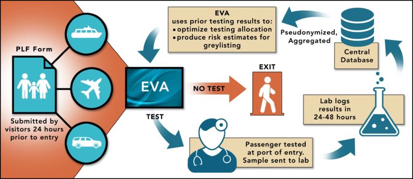
Introduction

In the first wave of the pandemic, many countries restricted non-essential travel to mitigate the spread of SARS-
CoV-2. The restrictions crippled most tourist economies, with estimated losses of 1 trillion USD among European
countries and 19 million jobs [3]. As conditions improved from April to July, countries sought to partially lift
these restrictions, not only for tourists, but also for the flow of goods and labor.

Different countries adopted different border screening protocols, typically based upon the origin country of the
traveler. Despite their variety, we group the protocols used in early summer 2020 into 4 broad types:
 • Allowing unrestricted travel from designated “white-list” countries.
 • Requiring travelers from designated “grey-listed” countries to provide proof of a negative RT-PCR test
 before arrival.
 • Requiring all travelers from designated “red-listed” countries to quarantine upon arrival.
 • Forbidding any non-essential travel from designated “black-listed” countries.

Most nations employed a combination of all four strategies. However, the choice of which “color” to assign to a
country differed across nations. For example, as of July 1st, 2020, Spain designated the countries specified in [1]
as white-listed, Croatia designated these countries as grey-listed or red-listed.

To the best of our knowledge, in all European nations except Greece, the above “color designations” were entirely
based on population-level epidemiological metrics (e.g., see [1, 2]) such as cases per capita, deaths per capita,
and/or positivity rates that were available in the public domain [4, 5, 6]. (An exception is the UK, which engaged
in small-scale testing at select airports that may have informed their policies.) However such metrics are
imperfect due to underreporting [7], symptomatic population biases [8, 9] and reporting delays.

These drawbacks motivated our design and nation-wide deployment of Eva: the first fully algorithmic, real-time,
reinforcement learning system for targeted COVID-19 screening with the dual goals of identifying asymptomatic,
infected travelers and providing real-time information to policymakers for downstream decisions.

The Eva System: Overview

Eva as presented here was deployed across all 40 points of entry to Greece, including airports, land crossings, and
seaports from August 6th to November 1st. Fig. 1 schematically illustrates its operation; Fig. 7 in Methods provides
a more detailed schematic of Eva’s architecture and data flow.

1. Passenger Locator Form (PLF)
All travelers must complete a PLF (one per household) at least 24 hours prior to arrival, containing (among other
data) information on their origin country, demographics, point and date of entry. [10] describes the exact fields
and how these sensitive data were handled securely.

2. Estimating Prevalence among Traveler Types
We estimate traveler-specific COVID-19 prevalence using recent testing results from previous travelers through
Eva. Prevalence estimation entailed two steps: First, we leverage LASSO regression from high-dimensional
statistics [11] to adaptively extract a minimal set of discrete, interpretable traveler types based on their
demographic features (country, region, age, gender); these types are updated on a weekly basis using recent testing
results. Second, we use an empirical Bayes method to estimate each type’s prevalence daily. Empirical Bayes has
previously been used in the epidemiological literature to estimate prevalence across many populations [12, 13].
In our setting, COVID-19 prevalence is generally low (e.g., ~2 in 1000), and arrival rates differ substantively

 Page 2 of 14

across countries. Combined, these features cause our testing data to be both imbalanced (few positive cases among
those tested) and sparse (few arrivals from certain countries). Our empirical Bayes method seamlessly handles
both challenges. Estimation details are provided in Section 2.2 of Methods.

Figure 1: Eva: A Reinforcement Learning System for COVID-19 Testing. Arriving passengers submit travel and demographic information 24
hours prior to arrival. Based on these data and testing results from previous passengers, Eva selects a subset of passengers to test. Selected
passengers self-isolate for 24-48 hours while labs process samples. Positive passengers are then quarantined and contact tracing begins; negative
passengers resume normal activities. Results are used to update Eva to improve future testing and maintain high-quality estimates of prevalence
across traveler subpopulations.

3. Allocating Scarce Tests
Leveraging these prevalence estimates, Eva targets a subset of travelers for (group) PCR testing upon arrival based
solely on their type, but no other personal information. The Greek National COVID-19 Committee of Experts
approved group (Dorfman) testing [14] in groups of 5 but eschewed larger groups and rapid testing due to concerns
over testing accuracy.

Eva’s targeting must respect various port-level budget and resource constraints that reflect Greece’s testing supply
chain, which included 400 health workers staffing 40 points of entry, 32 laboratories across the country, and
delivery logistics for biological samples. These constraints were (exogenously) defined and adjusted throughout
the summer by the General Secretariat of Public Health.

The testing allocation decision is entirely algorithmic and balances two objectives: First, given current
information, Eva seeks to maximize the number of infected asymptomatic travelers identified (exploitation).
Second, Eva strategically allocates some tests to traveler types for which it does not currently have precise
estimates in order to better learn their prevalence (exploration). This is a crucial feedback step. Today’s allocations
will determine the available data in Step 2 above when determining future prevalence estimates. Hence, if Eva
simply (greedily) sought to allocate tests to types that currently had high prevalence, then, in a few days, it would
not have any recent testing data about many other types that had moderate prevalence. Since COVID-19
prevalence can spike quickly and unexpectedly, this would leave a “blind spot” for the algorithm and pose a
serious public health risk. Such allocation problems can be formulated as multi-armed bandits [15, 16, 17, 18] –
which are widely studied within the reinforcement learning literature – and have been used in numerous

 Page 3 of 14

applications such as mobile health [19], clinical trial design [20], online advertising [21], and recommender
systems [22].

Our application is a nonstationary [23, 24], contextual [25], batched bandit problem with delayed feedback [26,
27] and constraints [28]. Although these features have been studied in isolation, their combination and practical
implementation poses unique challenges. One such challenge is accounting for information from “pipeline” tests
(allocated tests whose results have not yet been returned); we introduce a novel algorithmic technique of certainty-
equivalent updates to model information we expect to receive from these tests, allowing us to effectively balance
exploration and exploitation in nonstationary, batched settings. To improve interpretability, we build on the
optimistic gittins index for multi-armed bandits [29]; each type is associated with a deterministic index that
represents its current “risk score”, incorporating both its estimated prevalence and uncertainty. Algorithm details
are provided in Section 2.3 of Methods.

4. Grey-Listing Recommendations
Eva’s prevalence estimates are also used to recommend particularly risky countries to be grey-listed, in
conjunction with the Greek COVID-19 taskforce and the Presidency of the Government. Grey-listing a country
entails a tradeoff: requiring a PCR test reduces the prevalence among incoming travelers, however, it also reduces
non-essential travel significantly (approximately 39%, c.f. Sec. 5 of Methods), because of the relative
difficulty/expense in obtaining PCR tests in summer 2020. Hence, Eva recommends grey-listing a country only
when necessary to keep the daily flow of (uncaught) infected travelers at a sufficiently low level to avoid
overwhelming contact-tracing teams [30]. Ten countries were grey-listed over the summer of 2020 (see Sec. 5 of
Methods).

Unlike testing decisions, our grey-listing decisions were not fully algorithmic, but instead involved human input.
Indeed, while in theory, one might determine an “optimal” cut-off for grey-listing to balance infected arrivals and
reduced travel, in practice it is difficult to elicit such preferences from decision-makers directly. Rather, they
preferred to retain some flexibility in grey-listing to consider other factors in their decisions.

5. Closing the Loop
Results from tests performed in Step 3 are logged within 24-48 hours, and then used to update the prevalence
estimates in Step 2.

To give a sense of scale, during peak season (August and September), Eva processed 41,830 (±12,784) PLFs
each day, and 16.7% (± 4.8%) of arriving households were tested each day.

Results

Value of Targeted Testing: Cases Identified

We first present the number of asymptomatic, infected travelers caught by Eva relative to random surveillance
testing, i.e., where every arrival at a port of entry is equally likely to be tested. Random surveillance testing was
Greece’s initial proposal and is very common, partly because it requires no information infrastructure to
implement. However, we find that such an approach comes at a significant cost to performance (and therefore
public health).

We perform counterfactual analysis using inverse propensity weighting (IPW) [31, 32], which provides a model-
agnostic, unbiased estimate of the performance of random testing.

 Page 4 of 14

Season Improvement
 Peak 1.85x

 No. Infections Caught (Anonymized)
 Off−Peak 1.36x

 Sep Oct Nov

Figure 2: Comparing Eva vs. Randomized Surveillance Testing. Infections caught by Eva (red) vs estimated number of cases caught by random
surveillance testing (teal). The peak (resp. off-peak) season is Aug. 6 to Oct. 1 (resp. Oct. 1 to Nov. 1) and is denoted with triangular (resp.
circular) markers. Seasons are separated by the dotted line. Solid lines denote cubic-spline smoothing with 95% confidence intervals in grey.

During the peak tourist season, we estimate that random surveillance testing would have identified 54.1% (±8.7%)
of the infected travelers that Eva identified. (For anonymity, averages and standard deviations are scaled by
a (fixed) constant, which we have taken without loss of generality to be the actual number of infections
identified by Eva in the same period for ease of comparison.)

In other words, to achieve the same effectiveness as Eva, random testing would have required 85% more tests at
each point of entry, a substantive supply chain investment. In October, when arrival rates dropped, the relative
performance of random testing improved to 73.4% (±11.0%) (see Fig. 2). This difference is largely explained by
the changing relative scarcity of testing resources (see Fig. 3). As arrivals dropped, the fraction of arrivals tested
increased, thereby reducing the value of targeted testing. Said differently, Eva’s targeting is most effective when
tests are scarce. In the extreme case of testing 100% of arrivals, targeted testing offers no value since both random
and targeted testing policies test everyone. See Sec. 3 of Methods for details.

 Page 5 of 14

Season Tested
 Peak 18.43%
 Off−Peak 31.01%

 4x

 Performance Ratio

 2x

 0x

 20% 40% 60%
 Fraction Tested
Figure 3. Relative Efficacy of Eva over Random Surveillance vs. Fraction Tested. Ratio of number of infections caught by Eva relative to
number of (estimated) infections caught by random surveillance testing, as a function of the fraction of tested travelers. Dotted (resp. dashed)
line indicates the average fraction tested during the peak (resp. off-peak) tourist season. Triangular (circular) markers denote estimates from
peak (off-peak) days. Solid blue line denotes cubic-spline smoothing with a 95% confidence interval in grey.

Value of Reinforcement Learning: Cases Identified

We now compare to policies that require similar infrastructure as Eva, namely PLF data, but instead target testing
based on population-level epidemiological metrics (e.g., as proposed by the EU [2]) rather than reinforcement
learning. The financial investments of such approaches are similar to those of Eva, and we show these policies
identify fewer cases. (Sec. 3.2.3 of Methods highlights additional drawbacks of these policies, including poor data
reliability and a mismatch in prevalence between the general population and asymptomatic traveler population.)

We consider three separate policies that test passengers with probability proportional to either (i) cases per capita,
(ii) deaths per capita, or (iii) positivity rates for the passenger’s country of origin [4, 5, 6], while respecting port
budgets and arrival constraints. We again use IPW to estimate counterfactual performance (see Fig. 4).

 Page 6 of 14

Method Peak Off−Peak
 Cases 1.45x 1.09x

 No. Infections Caught (Anonymized)
 Deaths 1.37x 1.13x
 Positivity 1.25x 1.14x

 Aug Sep Oct Nov

 Cases Deaths Eva Positivity

Figure 4: Comparing Eva to Policies based on Epidemiological Metrics. Lines represent cubic-spline smoothing of daily infections caught for
each policy; raw points only shown for Eva and the “Cases” policy for clarity. The dotted line separates the peak (Aug. 6 to Oct. 1) and off-peak
(Oct. 1 to Nov. 1) tourist seasons.

During the peak tourist season (August, September), we found that policies based on cases, deaths and positivity
rates identified 69.0% (±9.4%), 72.7% (±10.6%), and 79.7% (±9.3%) respectively of the infected travelers
that Eva identified per test. In other words, Eva identified 1.25x – 1.45x more infections with the same testing
budget and similar PLF infrastructure. In October, when arrival rates dropped, the relative performance of
counterfactual policies based on cases, deaths and positivity rates improved to 91.5% (±11.7%), 88.8% (±10.5%)
and 87.1% (±10.4%) respectively. Like our results in the previous section, we find that the value of smart
targeting is larger when testing resources are scarcer. In fact, Eva’s relative improvement over these policies was
highest in the second half of the peak season (when infection rates were much higher and testing resources were
scarcer). See Sec. 3 of Methods for details.

Sec. 4 of Methods discusses possible reasons underlying the poor performance of simple policies based on
population-level epidemiological metrics, including reporting delays and systematic differences between the
general and asymptomatic traveler populations.

Poor Predictive Power of Population-Level Epidemiological Metrics

Given the poor performance of simple policies based on population-level epidemiological metrics, a natural
question is whether more sophisticated functions of these metrics would perform better. Although it is difficult to
eliminate this possibility, we argue this is likely not the case by studying a related question: “To what extent can
population-level epidemiological metrics be used to predict COVID-19 prevalence among asymptomatic travelers
as measured by Eva?” To the best of our knowledge, this is the first study of this kind. Surprisingly, our findings
suggest that widely used epidemiological data are generally ineffective in predicting the actual prevalence of
COVID-19 among asymptomatic travelers (the group of interest for border control policies).

Specifically, we examine the extent to which these data can be used to classify a country as high-risk (more than
0.5% prevalence) or low-risk (less than 0.5% prevalence); such a classification informs whether a country should

 Page 7 of 14

be grey- or black-listed. (A cutoff of 0.5% was typical for initiating grey-listing discussions with the Greek
COVID-19 taskforce, but our results are qualitatively similar across a range of cutoffs.) We compute the true
label for a country at each point in time based on Eva’s (real-time) estimates. We then train several models using
a Gradient Boosted Machine (GBM) [33] on different subsets of covariates derived from the 14-day time series
of cases per capita, deaths per capita, testing rates per capita, and testing positivity rates. Fig. 5 summarizes their
predictive accuracy; we obtained similar results for other state-of-the art machine learning algorithms.

 1.00
 Model AUROC
 1 0.504
 2 0.523
 3 0.518
 0.75 4 0.515
 True Positive Rate

 5 0.622

 0.50
 Model 1

 Model 2

 Model 3
 0.25
 Model 4

 Model 5

 0.00

 0.00 0.25 0.50 0.75 1.00
 False Positive Rate
Figure 5: Predictive Power of Publicly Reported Epidemiological Metrics. Each of Models 1-4 uses a different subset of features from: 14-day
time series of cases per capita, deaths per capita, tests performed per capita, and testing positivity rate. Model 5 additionally includes country
fixed-effects to model country-level idiosyncratic behavior. Models 1-4 are essentially no better than random prediction, while Model 5
achieves slightly better performance. See Sec. 4.1 of Methods for details on model construction and features used in each model.

Note that a random model that uses no data has an AUROC of 0.5. Thus, Models 1-4 offer essentially no predictive
value, suggesting that these population-level epidemiological data are not informative of prevalence among
asymptomatic travelers.

Model 5, which additionally uses country-level fixed effects, offers some improvement. These fixed effects
collectively model country-specific idiosyncrasies representing aspects of their testing strategies, social distancing
protocols and other non-pharmaceutical interventions that are unobserved in the public, epidemiological data. The
improvements of Model 5 suggests that these unobserved drivers are critical to distinguishing high- and low-risk
countries.

Overall, this analysis not only raises concerns about travel protocols proposed by the EU [2] based solely upon
widely used epidemiological metrics, but also about any protocol that treats all countries symmetrically. Indeed,
the idiosyncratic effects of Model 5 suggest that the thresholds for deciding whether COVID-19 prevalence in
travelers from Country A is spiking may differ significantly from that of Country B. See Section 4.1 for details.

In Section 4.3 of Methods, we also study the information delay between a country’s publicly reported cases (the
most common metric) and prevalence among asymptomatic travelers from that country. We expect a lag because

 Page 8 of 14

of the time taken for symptoms to manifest, and reporting delays induced by poor infrastructure. We find a modal
delay of 9 days.

Value of Grey-Listing: Cases Prevented

Eva’s measurements of COVID-19 prevalence were also used to provide early warnings for high-risk regions, in
response to which Greece adjusted travel protocols by grey-listing these nations. We estimate that Eva prevented
an additional 6.7% (±1.2%) infected travelers from entering the country through its early grey-listing decisions in
the peak season; results in the off-peak season are similar. For privacy, we have expressed the benefit relative to
the number of infected travelers identified by Eva. See Sec. 5 of Methods for details.

Conclusions: Lessons Learned from Deployment and Design Principles

To the best of our knowledge, Eva was the first large-scale data-driven system that was designed and deployed
during the COVID-19 crisis. Leading up to and throughout deployment, we met twice a week with the COVID-
19 Executive Committee of Greece, an interdisciplinary team of scientists and policymakers. Through those
meetings, we gleaned several lessons that shaped Eva’s design and contributed to its success.

Design the algorithm around data minimization. Data minimization (i.e., requesting the minimum required
information for a task), is a fundamental tenet of data privacy and the General Data Protection Regulation (GDPR).
We met with lawyers, epidemiologists, and policymakers before designing the algorithm to determine what data
and granularity may legally and ethically be solicited by the PLF. Data minimization naturally entails a tradeoff
between privacy and effectiveness. We limited requests to features thought to be predictive based on best available
research at the time (origin, age and gender [34, 35]), but omitted potentially informative but invasive features
(e.g., occupation). We further designed our empirical Bayes estimation strategy around these data limitations.

Prioritize interpretability. For all parties to evaluate and trust the recommendations of a system, the system must
provide transparent reasoning. An example from our deployment was the need to communicate the rationale for
“exploration” tests, i.e., tests for types with moderate but very uncertain prevalence estimates). Such tests may
seem wasteful. Our choice of empirical Bayes allowed us to easily communicate that types with large confidence
intervals may have significantly higher risk than their point estimate suggests, and thus require some tests to
resolve uncertainty; see, e.g., Figs. 9 and 11 in Methods, which were featured on policymakers’ dashboards.

A second example was our choice to use gittins indices, which provide a simple, deterministic risk metric for each
type that incorporates both estimated prevalence and corresponding uncertainty, driving intuitive test allocations.
In contrast, using Upper Confidence Bound or Thompson Sampling with logistic regression [36, 37] would have
made it more difficult to visualize uncertainty (a high-dimensional ellipsoid or posterior distribution) and test
allocations would depend on this uncertainty through an opaque computation (a high-dimensional projection or
stochastic sampling).

This transparency fostered trust across ministries of the Greek Government using our estimates to inform
downstream policy making, including targeting contact-tracing teams, staffing of mobile testing units, and
adjusting social distancing measures.

Design for flexibility. Finally, since these systems require substantial financial and technical investment, they need
to be flexible to accommodate unexpected changes. We designed Eva in a modular manner disassociating type
extraction, estimation, and test allocation. Consequently, one module can easily be updated without altering the

 Page 9 of 14

remaining modules. For example, had vaccine distribution begun summer 2020, we could define new types based
on passengers’ vaccination status without altering our procedure for prevalence estimates or test allocation.
Similarly, if rapid testing were approved, our allocation mechanism could be updated to neglect delayed feedback
without affecting other components. This flexibility promotes longevity, since it is easier to get stakeholder buy-
in for small adjustments to an existing system than for a substantively new approach.

Bibliography
[1] Council recommendation on the temporary restriction on non-essential travel into the EU and the possible lifting of
 such restriction, Brussels, 30 June 2020: https://www.consilium.europa.eu/media/47592/st_9208_2020_init_en.pdf.
[2] Draft Council Recommendation on a coordinated approach to the restriction of free movement in response to the
 COVID-19 pandemic, Brussels, 12 October 2020: General Secretariat of the Council.
[3] "World Travel and Tourism Council," November 2020. [Online]. Available: Council
 https://wttc.org/Research/Economic-Impact/Recovery-Scenarios.
[4] J. Hasell, E. Mathieu, D. Beltekian, B. a. G. C. a. O.-O. E. Macdonald, M. Roser and H. Ritchie, "A cross-country
 database of COVID-19 testing," Scientific data, vol. 7, no. 1, pp. 1-7, 2020.
[5] M. Roser, H. Ritchie, E. Ortiz-Ospina and J. Hasell, "Coronavirus Pandemic (COVID-19)," OurWorldInData.org,
 2020. [Online]. Available: https://ourworldindata.org/coronavirus.
[6] E. Dong, H. Du and L. Gardner, "An interactive web-based dashboard to track COVID-19 in real time," The Lancet
 infectious diseases, vol. 20, no. 5, pp. 533-534, 2020.
[7] S. L. Wu, A. N. Mertens, Y. S. Crider, A. Nguyen, N. N. Pokpongkiat, S. Djajadi, A. Seth, M. S. Hsiang, J. M. J.
 Colford, A. Reingold, B. F. Arnold, A. Hubbard and J. Benjamin-Chung, "Substantial underestimation of SARS-
 CoV-2 infection in the United States," Nature Communications, 2020.
[8] C. Muge, T. Matthew, L. Ollie, A. E. Maraolo, J. Schafers and H. Antonia, "SARS-CoV-2, SARS-CoV, and MERS-
 CoV viral load dynamics, duration of viral shedding, and infectiousness: a systematic review and meta-analysis," The
 Lancet Microbe, 2020.
[9] S. Phipps, Q. Grafton and T. Kompas, "Robust estimates of the true (population) infection rate for COVID-19: a
 backcasting approach," Royal Society Open Science, vol. 7, no. 11, 2020.
[10] Ministry of Civil Protection and Ministry of Tourism, Hellenic Republic, "Protocol for Arrivals in Greece," [Online].
 Available: https://travel.gov.gr/#/policy.
[11] R. Tibshirani, "Regression shrinkage and selection via the lasso," Journal of the Royal Statistical Society: Series B
 (Methodological), pp. 267-288, 1996.
[12] S. Greenland and J. Robins, "Empirical-Bayes adjustments for multiple comparisons are sometimes useful,"
 Epidemiology, pp. 244-251, 1991.
[13] O. J. Devine, T. Louis and E. Halloran, "Empirical Bayes methods for stabilizing incidence rates before mapping,"
 Epidemiology, pp. 622-630, 1994.
[14] R. Dorfman, "The detection of defective members of large populations," The Annals of Mathematical Statistics, vol.
 14, no. 4, pp. 436-440, 1943.
[15] W. Thompson, "On the likelihood that one unknown probability exceeds another in view of the evidence of two
 samples," Biometrika, pp. 285-294, 1933.
[16] T. L. Lai and H. Robbins, "Asymptotically efficient adaptive allocation rules," Advances in applied mathematics, pp.
 4-22, 1985.
[17] J. Gittins, "Bandit processes and dynamic allocation indices," Journal of the Royal Statistical Society: Series B
 (Methodological), pp. 148-164, 1979.

 Page 10 of 14

[18] P. Auer, "Using confidence bounds for exploitation-exploration trade-offs," Journal of Machine Learning Research,
 pp. 397-422, 2002.
[19] A. Tewari and S. A. Murphy, "From Ads to Interventions: Contextual Bandits in Mobile Health," in Mobile Health,
 SpringerLink, 2017.
[20] A. Durand, C. Achilleos, D. Iacovides, K. Strati, G. D. Mitsis and J. Pineau, "Contextual bandits for adapting
 treatment in a mouse model of de novo carcinogenesis," in Machine Learning for Healthcare Conference, 2018.
[21] L. Li, W. Chu, J. Langford and R. Schapire, "A contextual-bandit approach to personalized news article
 recommendation," Proceedings of the 19th international conference on World wide web, pp. 6611-670, 2010.
[22] F. Amat, A. Chandrashekar, T. Jebara and J. Basilico, "Artwork personalization at Netflix," Proceedings of the 12th
 ACM conference on recommender systems, pp. 487-488, 2018.
[23] O. Besbes, Y. Gur and A. Zeevi, "Stochastic multi-armed-bandit problem with non-stationary rewards," Advances in
 neural information processing systems, pp. 199-207, 2014.
[24] H. Luo, C.-Y. Wei, A. Agarwal and J. Langford, "Efficient contextual bandits in non-stationary worlds," Conference
 on Learning Theory, pp. 1739-1776, 2018.
[25] H. Bastani and M. Bayati, "Online decision making with high-dimensional covariates," Operations Research, pp.
 276-294, 2020.
[26] Z. Gao, Y. Han, Z. Ren and Z. Zhou, "Batched multi-armed bandits problem," Advances in Neural Information
 Processing Systems, pp. 503-514, 2019.
[27] V. Perchet, P. Rigollet, S. Chassang and E. Snowberg, "Batched bandit problems," The Annals of Statistics, pp. 660-
 681, 2016.
[28] S. Agrawal and N. Devanur, "Bandits with concave rewards and convex knapsacks," Proceedings of the fifteenth
 ACM conference on Economics and computation, pp. 989-1006, 2014.
[29] E. Gutin and V. Farias, "Optimistic gittins indices," Advances in Neural Information Processing Systems, pp. 3153-
 3161, 2016.
[30] Hellewell, J.; Abbott, S.; Gimma, A.; Bosse, N. I.; Jarvis, C. I.; Russell, T. W.; Munday, J. D.; Kucharski, A. J.;
 Edmunds, W. J.; Centre for the Mathematical Modelling of Infectious Diseases COVID-19 Working Group; Funk,
 S.; Eggo, R. M., "Feasibility of controlling COVID-19 outbreaks by isolation of cases and contacts," The Lancet.
 Global health, 2020.
[31] W. G. Imbens and B. D. Rubin, Causal Inference in Statistics, Social and Biomedical Sciences, Cambridge
 University Press, 2015.
[32] P. Rosenbaum and D. Rubin, "The central role of the propensity score in observational studies for causal effects,"
 Biometrika, vol. 70, no. 1, pp. 41-55, 1983.
[33] Friedman, "Greedy function approximation: a gradient boosting machine," Annals of Statistics, pp. 1189-1232, 2001.
[34] N. Davies, P. Klepac and Y. Liu et al., "Age-dependent effects in the transmission and control of COVID-19
 epidemics," Nature Medicine, 2020.
[35] S. Davies and B. Bennet, "A gendered human rights analysis of Ebola and Zika: Locating gender in global health
 emergencies," International Affairs.
[36] S. Agrawal and N. Goyal, "Thompson sampling for contextual bandits with linear payoffs," in International
 Conference on Machine Learning, 2013.
[37] W. Chu, L. Li, L. Reyzin and R. Schapire, "Contextual bandits with linear payoff functions," in Conference on
 Artificial Intelligence and Statistics, 2011.

 Page 11 of 14

End Notes

Acknowledgements. The authors would like to thank all members of the Greek COVID-19 Taskforce, the Greek Prime
Minister Kyriakos Mitsotakis, the Ministry of Digital Governance, the General Secretariat for Civil Protection, the
Ministry of Health, the National Public Health Organization, the development team from Cytech as well as the border
control agents, doctors, nurses and lab personnel that contributed to Eva’s deployment. Furthermore, the authors would
like to thank Osbert Bastani for discussions and analysis on constructing custom risk metrics from public data. V.G.
was partially supported by the National Science Foundation through NSF Grant CMMI-1661732. We also thank the
Editor and 4 anonymous reviewers for their comments on an earlier draft of this manuscript.

Author Contributions. H.B., K.D., and V.G. constructed the model, designed and coded the algorithm, and performed
the analysis in this paper. J.V. designed the software architecture and APIs to communicate with the Central Database
of the Ministry of Digital Governance. C.H., P.L., G.M., D.P., and S.T. contributed to and informed epidemiological
modeling choices of the system. All authors coordinated Eva’s operations and logistics throughout its deployment.

Author Information. H.B., V.G., and J.V. declare no conflict of interest. K.D. declares non-financial competing
interest as an unpaid Data Science and Operations Advisor to the Greek Government from May 1st, 2020 to Nov 1st,
2020. C.H., P.L., G.M., D.P., and S.T. declare non-financial competing interest as members of the Greek National
COVID-19 Taskforce. Correspondence should be addressed to drakopou@marshall.usc.edu.

 Page 13 of 14

Data and Code Availability

Data availability. To support further research, aggregated, anonymized data are available
at https://github.com/kimondr/EVA_Public_Data. These data aggregate passenger arrival and testing information
over pairs of consecutive days, country of origin, and point of entry.

The finer granularity data that support the (exact) findings of this study are protected by GDPR. These data are
available from the Greek Ministry of Civil Protection but restrictions apply to the availability of these data, which
were used under license for the current study, and so are not publicly available. Access to these data can only be
granted by the Greek Ministry of Civil Protection (info@gscp.gr) for research that is conducted in the public interest
for public health (GDPR Recital 159) and scientific purposes (GDPR Article 89).

Finally, the population-level epidemiological metrics used in our analysis can be obtained freely from the “Our
World In Data COVID-19 dataset (https://github.com/owid/covid-19-data/tree/master/public/data).

Code Availability. All code used in this paper was written in a combination of R and Python 3.7 The code for the
deployment of the algorithm on a sample dataset is available at
https://github.com/vgupta1/EvaTargetedCovid19Testing. The code for reproducing the results of our counterfactual
analysis is available at https://github.com/vgupta1/Eva_CounterfactualAnalysis.

 Page 14 of 14

Methods

1 Problem Description

Notation and System Constraints

Let ∈ {1, … , } index time (in days), ∈ {1, … , ℰ} index points of entry, and ∈ {1, … , } index the
set of 193 countries from which travelers may originate. Moreover, for each point of entry , let ! ( )
denote the budget of available tests at time .

Pertinent demographic data about a passenger (extracted from their PLF) include their country and
region of origin, age group and gender. Since all extracted features are categorical, we represent them
with a finite, discrete set of values . We refer to passengers with features ∈ as -passengers.
Let "! ( ) denote the number of -passengers arriving with date of entry and point of entry . For
every ∈ , let " ( ) denote the unknown, time-varying, underlying prevalence among -
passengers, i.e., the probability that a -passenger is infected.

The budgets ! ( ) were exogenously determined by the Secretary General of Public Health. Note that
the availability of tests relative to arrivals varies significantly across points of entry (see Fig. 6).

Decision Problem

The primary decision problem on day is to choose the number of tests "! ( ) to allocate to -
passengers at point of entry . To formally define this problem, we first specify the information
available at time . Namely, let " ( ) and " ( ) denote the number of -passengers that tested positive
and negative at time , respectively. Then, since labs take up to two days to process testing results, the
available information on day is
 { " ( # ), " ( # )}" ∈ ,( !)(*+ .
Thus, at the beginning of day , we must determine the number of tests "! ( ) to be performed on -
passengers at point of entry using this information.

Furthermore, our testing decisions need to satisfy two constraints:
 ∑"∈ "! ( ) ≤ ! ( ), ∀ ∈ {1, … , ℰ}, (Budget Constraint),
ensuring that the number of allocated tests does not exceed the budget at each point of entry, and
 "! ( ) ≤ "! ( ), ∀ ∈ , ∈ {1, … , ℰ}, (Arrivals Constraint),
ensuring that the number of allocated tests for -passengers does not exceed the number of arriving -
passengers.

A secondary decision problem is to choose “color designations” for every country as described in the
main text. We denote the set of black, grey, and white-listed countries at time by ℬ( , ( , ( ,
respectively. Note that determining these sets must be done one week in advance (to provide notice to
travelers of possibly changing travel requirements). Hence the relevant sets to choose at time are
ℬ(,- , (,- , (,- .

 Page 1 of 32

Promachonas

 Kavala

 Thessaloniki

 Kerkyra

 Skiathos
 Mitilini
 Aktion

 Kefalonia Araxos
 Athens
 Zakinthos
 Mykonos

 Kalamata
 Kos

 10% Santorini Rhodes

 20%

 Chania
 50% Heraklion Karpathos

Figure 6: Testing Capacity at Selected Points of Entry. Circle icons denote airports; square icons denote seaports; triangle icons
denote land borders. Icon sizes indicate the fraction of daily arrivals that could be tested at each point of entry during the peak
season. Note that information on some points of entry is omitted due to the sensitive nature of the data. Basemap obtained from R-
package ‘maps’ under GNU General Public License, version 2 (GPLv2).

As discussed, unlike our testing decisions, color designation decisions are not entirely algorithmic.
Rather, they were made in conjunction with the Greek COVID-19 taskforce, and further
reviewed/authorized by the Office of the Prime Minister.1 In particular, Eva was only used to identify
candidates for grey-listing based on its estimates of the current prevalence " ( ). In what follows, we
focus on the algorithmic elements of our procedure, i.e., determining "! ( ) and, as part of that process,
estimating " ( ).

Objective
Note that, conditional on "! ( ), the number of positive tests observed at entry is binomially
distributed with "! ( ) trials and (unknown) success probability " ( ). Our goal is to maximize the
expected total number of infections caught at the border, i.e.,
 ℰ

 @A A A "! ( ) " ( )B.
 (/0 " ∈ !/0

Note that the testing decisions we make at time affect the information that will be available in the
future, and thereby the quality of our prevalence estimates C D" ( ′)F" ∈ for # > .

Thus, when deciding "! ( ), we must balance two seemingly conflicting objectives. On the one hand,
a myopic decision-maker would allocate tests to the (estimated) riskiest passengers, based on their

1
 For completeness, we summarize Greece’s color designation process as follows: Greece adopted the European
Union’s recommended black-list designations ℬ!"# ; all non-Greek citizens from black-listed countries were forbidden
entry, and 100% of Greek citizens arriving from black-listed countries were tested at the border. Of the remaining
countries (which accounted for over 97% of arrivals), Greece designated a small subset as grey-listed countries ( !"# )
if current prevalence was deemed sufficiently high (see Table 19 in Sec. 5 for list of countries), and the remainder as
white-listed countries ( !"# ).

 Page 2 of 32

features and our current prevalence estimates C D" ( )F. On the other hand, a forward-looking
decision-maker would want to collect data on -passengers for every value of , in order to make
accurate future assessments on which passengers are risky. This suggests allocating tests uniformly
across feature realizations to develop high-quality surveillance estimates.

This tension – known as the exploration-exploitation tradeoff – is well-studied in the multi-armed
bandit literature [1, 2, 3]. Optimal solutions balance the need to explore (accurately learn the current
prevalence " ( ) for all ) and to exploit (use the estimated prevalence C D" ( )F" ∈ to allocate tests
to the riskiest passengers).

2 Algorithm Description

2.1 Overview of Algorithm

The tradeoff presented in Section 1 resembles a multi-armed bandit problem. However, our setting
exhibits a number of salient features that distinguish it from the classical formulation:

 1. Non-stationarity: The prevalence " ( ) is time-varying.
 2. Imbalanced Data: On average, only 2 in 1000 passengers tests positive, meaning the data
 { " ( # ), " ( # )}" ∈ ,( !)(*+ is very imbalanced with mostly negative tests.
 3. High-Dimensionality: The number of possible features is very large.
 4. Batched decision-making: All testing allocations for a day must be determined at the start of
 the day (batch) for each point of entry.
 5. Delayed Feedback: Labs may take up to 48 hours to return testing results.
 6. Constraints: Each point of entry is subject to its own testing budget and arrival mix.

Although these features have been studied in isolation, their combination poses unique challenges. We
next propose a novel algorithm that addresses these features in our setting. We separate our
presentation into two parts: estimation and allocation. Our estimation procedure (Section 2.2) builds
on ideas from empirical Bayes and high-dimensional statistics to address the challenges of non-
stationarity, imbalanced data and high-dimensionality. Our allocation procedure (Section 2.3) uses
these estimates and adapts classical multi-arm bandit algorithms to address the challenges of batched
decision-making, delayed feedback, and budget constraints.

Before delving into details, we note that to address the aforementioned high-dimensionality, we
periodically partition the set of features into types, denoted by ( . On first reading the reader can
take a passenger’s type to be equivalent to their country of origin (i.e., ignoring more granular feature
information such as origin region, age and gender) without much loss of meaning. However, in reality,
we distinguish particularly risky passenger profiles within a country as additional, distinct types, where
these “risky profiles” are identified dynamically using LASSO regression with recent testing results
(see Section 2.2 for details). Over time, as new testing data arrives, we update this partition, yielding a
time-dependent set of types ( . We treat all -passengers of the same type ∈ ( symmetrically in
our estimation and allocation procedures, i.e., our estimates satisfy ̂"" ( ) = ̂"# ( ) for all features
 0 , + ∈ . This process reduces the dimensionality of our estimation and allocation problems from
| | to | ( |.

 Page 3 of 32

Fig. 7 overviews the architecture and data flow of Eva.

Figure 7: The Data Flow of Eva. The core algorithmic components of Eva are depicted by shaded boxes. All data flows, including
personal data obtained via the PLF, were managed by the Greek Government (see [4]). Adaptive types were updated once per
week and held constant between updates. Throughout the summer, our algorithm only identified adaptive types based on the country
and region; types were never defined based on age group and gender (see also Section 2.2 below).

2.2 Estimation

In this section, we focus on developing estimates for prevalence rates 2 ( ) for a given day ; we drop
the time index when it is clear from context.

Recall that the (unknown) prevalence rates 2 ( ) are time-varying. Common strategies for estimation
in time-varying settings include discarding sufficiently old data [5, 6] or exponential smoothing [7].
The kernel smoothing literature [8] suggests that discarding old data might be preferred if the rates
 2 ( ) are particularly non-smooth in time. Based on this intuition and conversations with
epidemiologists on Greece’s COVID-19 taskforce, we choose to discard testing results that are more
than 16 days old. As before, let
 (*3

 2 = A 2 ( # ),
 ( ! /(*04

denote the total number of type passengers that tested positive over the past 14 days of test results,
and let
 (*3

 2 = A 2 ( # ),
 ( ! /(*04

denote the total number of type passengers that tested negative over the past 14 days of test results.
An unbiased, and natural estimate of the prevalence for type is
 2
 ̂25678! = . (1)
 2 + 2

 Page 4 of 32

However, because prevalence rates are low (on the order of 2 in a 1000), the variability of this estimator
is on the same order as 2 ( ) for moderate values of 2! ( ). Worse, for rare types where 2! ( ) is
necessarily small (e.g., less than 100 arrivals in last 16 days), the variability is quite large. This high
variability often renders the estimator unstable/inaccurate, an observation also recognized by prior
epidemiological literature [9, 10].

As a simple illustration, consider a (foolish) baseline estimator that estimates every prevalence to be
zero. We compute this baseline estimator and the naïve estimator in Eq. (1) for all countries as of
September 1, 2020. We find that the average MSE (averaged over countries) of the naïve estimator is
larger than that of the baseline estimator (see Fig. 8 below). In fact, a conservative estimate of the error
of ̂25678! is
 OExcess MSE of ̂25678! over Baseline = √. 000334 = 0.018,

which is larger than the typical prevalence of most countries. In other words, any potential signal is
entirely washed out by noise.

 0.00012

 0.00008
 Excess MSE

 0.00004

 0.00000

 0 100 200 300 400 500
 Prior Strength (α + β)
Figure 8: Excess MSE over Baseline Estimator. The baseline estimates zero prevalence for all types. The naïve estimator
(clipped from the plot for readability) corresponds to a prior strength of zero and has far worse MSE than the baseline. Our
empirical Bayes estimator (red dot) substantively improves performance and approximately minimizes MSE by trading off bias
and variance.

To compensate for high variability and potentially rare types, we adopt an empirical Bayes perspective.
This improves the stability of our estimates at the expense of introducing some bias. Our approach
naturally allows information-sharing across types, so that rare types partially borrow data from other
similar types to improve their stability.

At a high level, our estimation procedure has two steps: First, for each color designation (white, grey
or black-listed) ∈ { ( , ( , ( }, we fit a prior Beta(α9 ( ), β9 ( )) for all types from countries of that
color-designation. Second, we compute Bayesian (posterior) estimates for each 2 ( ), assuming 2 ( )
was drawn from the appropriately colored prior.

Specifically, consider countries of color ∈ { ( , ( , ( }, and the corresponding set of types ℒ9 = { ∈
 ( ∶ is from a country in l}. Let 2 = 2 + 2 be the total number of tests (with results) allocated to

 Page 5 of 32

type over the last 16 days. Conditional on 2 , 2 is approximately binomially distributed with 2
trials and success probability 2 . If we further assume that for each ∈ ℒ9 , 2 was drawn
independently from a Beta( : , β9 ) distribution, then the strong law of large numbers yields:
 1 2 6.=. 1 2 1 9
 A mn A o | 2 p = A [ 2 ] =
 |ℒ9 | 2 |ℒ9 | 2 |ℒ9 | 9 + 9
 2∈ℒ$ 2∈ℒ$ 2∈ℒ$

and
 1 2 ( 2 − 1) 6.=. 1 2 ( 2 − 1)
 A mn A u | v
 |ℒ9 | 2 ( 2 − 1) |ℒ9 | 2 ( 2 − 1) 2
 2∈ℒ$ 2∈ℒ$
 1 +
 l+ l l
 = ]
 A [ 2 = + ,
 |ℒ9 | ( l + l ) + ( l + 9 ) + ( l + l + 1)
 2∈ℒ$

where the limits are taken as |ℒ9 | → ∞. Taking the left sides of the above two expressions as estimators
for the right sides, we can rearrange to find estimates of (α9 , β9 ), yielding
 +
 09 (1 − 09 )
 α
 y: = + + − 09
 +9 − 09
 (1 − 09 )
 βD: = α
 y:
 09
 1 2
 09 = A (2)
 |ℒ9 | 2
 2∈ℒ$

 1 2 ( 2 − 1)
 +9 = A (3)
 |ℒ9 | 2 ( 2 − 1)
 2∈ℒ$

We repeat this procedure separately for each of the three-color designations. Equipped with these
priors, we then compute posterior distributions for each type ∈ ℒ9 . By conjugacy, these
are Beta(α> , β> ) distributed with estimates
 α y9 + P2 and €2 = €9 + 2 ,
 y2 = α
suggesting the following empirical Bayes estimate of the prevalence 2 :
 α
 y2
 ̂2?@ = . (4)
 y2 + €2
 α
To provide intuition, notice that if type comes from a country with color designation , our posterior
estimate can be rewritten as
 2 α9 2
 ̂2?@ = •1 − ‚ + ̂ 5678! ,
 2 + 9 + 9 α9 + 9 2 + 9 + 9 2
i.e., it is a weighted average between the naïve prevalence estimator and our prior mean. The sum
(α9 + 9 ) is often called the strength of the prior. For rare types where 2 is small relative to (α9 + 9 ),
the estimator is close to the prior mean (i.e., it draws information from similar types). For common
types where 2 is large relative to (α9 + 9 ), it is close to the naïve estimator (i.e., it lets the type’s own
testing data speak for itself). This structure matches our intuition that the naive estimator should only
be used when 2 is large enough.

 Page 6 of 32

Below, we summarize the estimation strategy.
 Subroutine 1: Estimating Prevalence via Empirical Bayes
 Input: # of positives 2 , negatives 2 and tests 2 for each type in the past 14 days of test results.

 for each color designation of countries ∈ { ( , ( , ( }
 Compute 09 , +9 from Eq. (2) and (3)
 +
 09 (1 − 09 ) (1 − 09 )
 α
 y9 ← + + − 09 , βD9 ← α
 y9
 +9 − 09 09
 for all types ∈ ℒ9 whose origin country is in :
 α
 y2 ← αy9 + 2 and €2 ← βD9 + 2
 end
 end

Fig. 8 shows the excess MSE for various estimators with differing strength in the prior (the naïve
estimator ̂25678! corresponds to a prior strength of zero and its MSE is too large to fit on the plot). Our
moment-matching estimator (red dot) approximately minimizes the MSE while maintaining a tractable
closed-form expression.

2.2.1 Reducing Dimensionality through Adaptive Type Extraction

As mentioned earlier, we adaptively partition the discrete space of features into a smaller set of types
 ( to reduce the dimensionality of the problem. Defining types entirely by a passenger’s country of
origin is attractive for its operational simplicity and because geography is highly predictive of
prevalence. That said, there can be significant heterogeneity in infection prevalence based on other
passenger feature information. For example, certain regions within a country may have a high
population density and low social distancing compliance relative to the rest of the country, resulting in
a much higher risk for passengers originating from that region; certain age brackets or genders may
also carry higher risk. Defining types solely at the country-level risks poor test allocations by failing
to test passengers with features that suggest high risk.

Consequently, our dimensionality reduction procedure starts with types defined at the country level,
but then goes one step further to distinguish particularly risky passengers based on their feature
information (origin region and demographic characteristics) as additional, distinct types.2 These
additional types are identified dynamically based on recent testing results and allow us to exploit intra-
country heterogeneity in prevalence to better allocate testing resources.

We identify additional types using the celebrated LASSO procedure [11], which has also previously
been used for dimensionality reduction in contextual bandits [12]. Specifically, we first apply our
previous empirical Bayes estimation strategy assuming country-based types. Given these estimates, we
then perform a LASSO logistic regression on the last 14 days of testing results, where the unit of
observation is a single passenger’s test, and features include (1) the estimated prevalence ̂2?@ of the

2
 Regions indicates more granular locations within a country (e.g., state or province). Since different countries use
different nomenclature, we use the generic term “region.”

 Page 7 of 32

passenger’s origin country (estimated in previous step), (2) indicator variables for potential regions,
(3) indicator variables for gender-country pairs and (4) indicator variables for age-country pairs. As
will become clear below, we interact gender and age with the country of origin since our goal is to
further split existing country-level types based on demographic information, as warranted by the data.

Mathematically, let denote a tested passenger (from the last 14 days of testing results), 7 ∈ {0, 1}
denote their binary test result, 7 denote their origin country, 7 denote their origin region, 7 denote
their gender-country pair (i.e., the cross product of their gender and country categorical variables), and
 7 denote their age-country pair (i.e., the cross product of their age group and country categorical
variables). We then perform the LASSO logistic regression:

 7 = A ̂A?@
 %
 + A B { = 7 } + A C { = 7 } + A 6 { = 7 } + 7 (5)
 B C 6

Let the number of unique countries from the last two weeks be , the number of unique regions from
the last two weeks be , and further note that there are 3 gender options and 10 possible age brackets.
Then, the total number of features is 1 + 13 + . Note that and change over time as a function
of the types of recent arrivals; we typically had scheduled arrivals from ≈ 170 countries and roughly
 ≈ 17,000 cities. The regression above yields a sparse vector of coefficients ‘ €A , €B , €C , €6 ’. These
coefficients indicate types of passengers whose estimated prevalence (based on their feature
information) is notably different than their estimated prevalence based solely on their origin country,
based on recent testing data. We are primarily interested in identifying risky passenger types (so we
can concentrate our limited testing resources on such passengers). Hence, we only introduce new
type(s) when we identify positive coefficients in the support.

As a clarifying example, if a region has a corresponding positive €B , then the prevalence of
passengers from region have notably higher prevalence than passengers of its corresponding country
 . Thus, we define a new type for passengers originating from , but also retain a type for passengers
originating from that are not from . We apply similar transformations for other positive coefficients
in the LASSO regression as well.

Interestingly, during the summer of 2020, we always found that €C = 0 for all gender-country pairs
and €6 = 0 for all age-country pairs, i.e., we never found the age bracket and/or gender to be predictive
of passenger test results beyond country/region of origin. This non-predictive behavior is likely
because only one member of a household fills out the PLF (using their own age and gender) but the
household likely spans members of different ages and genders. Note that the constraint of one PLF per
household was a hard constraint imposed by Greek government.

The process is summarized below in Subroutine 2. For simplicity, we have only stated the algorithm
in the case of potentially positive elements in €B , since we never found other features to be predictive.

Subroutine 2: Adaptive Type Extraction
Input: 7 , 7 , 7 # historical test results with country and region dummies
Perform Lasso regression according to Eq. (5)
return set of types ( = {1, … , } ∪ ” 7 : ‘ €B ’7 > 0–

 Page 8 of 32