Energy-Agile Laptops: Demand Response of Mobile Plug Loads Using Sensor/Actuator Networks
←
→
Page content transcription
If your browser does not render page correctly, please read the page content below
Energy-Agile Laptops: Demand Response of Mobile
   Plug Loads Using Sensor/Actuator Networks
                Nathan Murthy†∧ , Jay Taneja‡ , Kamil Bojanczyk? , David Auslander∧ , and David Culler‡

       † Cloud-basedSolutions Innovation Group, Fujitsu Laboratories of America, Sunnyvale, California 94085
              ‡ ComputerScience Division, University of California, Berkeley, Berkeley, California 94720
                       ? College of Engineering, Cornell University, Ithaca, New York 14850
       ∧ Department of Mechanical Engineering, University of California, Berkeley, Berkeley, California 94720

 Email: nathan.murthy@us.fujitsu.com, {taneja,culler}@cs.berkeley.edu, ksb37@cornell.edu, dma@me.berkeley.edu

   Abstract—This paper explores demand response techniques          themselves for new market segments. We investigate laptops
for managing mobile, distributed loads with on-board elec-          in this paper because of their mobile energy storage features
trochemical energy storage over a plug-level sensing/actuating      and because of their ubiquity in daily life. Energy storage
wireless mesh network. We target laptops and construct a power
consumption and battery charging model from measurements            gives them unique load deferment properties; but since laptop
obtained across a variety of such devices. We then build sim-       battery charging is random and mobile (it is hard to predict
ulations of charging patterns using the most general cases we       when and where someone will charge a laptop from an outlet),
observed. Our first simulation study explores a classic demand      managing several of these devices as one aggregate load from
response scenario in which a large number of loads participate      a DR perspective poses unique challenges.
in a typical pre-scheduled demand response (DR) event. We
show that we can achieve load curtailments in the range of 30-         The work we present herein has many parallels with the
90% of aggregate baseline load as a function of the duration        electric vehicle (EV) charging problem. As utilities and grid
of a DR event by managing the charging schedules of laptops         operators anticipate more EVs hitting markets, the use case
that randomly enter and leave the control jurisdiction of a DR      of DR for laptops serves as a proxy for the looming question
event participant. In a second simulation study, we investigate a   of how to manage EV charging schedules in a DR setting.
continuous demand response scenario in which charging schedules
respond to a fluctuating renewable electricity supply (e.g. wind    We build on the existing literature on EV charging [11],
or solar) and show that we can reduce grid dependence by 26.8-      [12], [13] and address some of the burgeoning challenges
33.8% compared to oblivious charging.                               facing consumer groups who are becoming empowered and
                                                                    interconnected through new energy production technologies.
           I. I NTRODUCTION AND BACKGROUND
   The motivation for creating demand response (DR) solutions                      II. L APTOP C HARGING M ODEL
for buildings at the plug-load level comes at a moment when            Our models fundamentally rely on understanding the power
growing interest in building energy science research [1], [2]       consumption profiles of laptops as a function of their capacities
coincides with increasing maturity in load-monitoring wireless      or states of charge (SoC). It is already well known that as
sensor network deployments [3]. Research in built environ-          the charge in a lithium-ion battery is depleted, the resistance
ment sciences has been making significant strides in energy         within the battery increases and therefore the amount of power
efficiency as well as in DR. In some cases, whole buildings         delivered to a battery in a low SoC is higher than the amount
have been transformed into state-of-the art laboratories for        of power delivered to a battery in a high SoC. It is also
experimenting DR strategies and for collecting submetered           well known that the charging dynamics and capacity limits
energy usage data from building-level to plug-level resolution      of rechargeable batteries vary over their lifetimes depending
[4]. Progress in large-scale, long-term wireless sensor/actuator    on the nature of their charge and discharge cycles. Without
networks makes it possible to monitor and manage plug loads         even introducing vendor-specific laptop designs, these simple
in very dynamic building environments [5], [6]. Moreover,           facts about laptop batteries alone imply that our problem cuts
microgrid projects around the world in remote areas present         across a great deal of heterogeneity which makes this problem
emerging challenges to fulfilling the energy needs of whole         particularly interesting from a characterization standpoint.
communities moving towards energy independence or of those             In general, we can classify laptops as either having or
who depend almost entirely on intermittent generation [7], [8]      lacking charge control mechanisms. These built-in charge con-
as their only source of electricity.                                trollers, or lack thereof, affect the individual power consump-
   Demand response presents opportunities to explore novel          tion patterns aggregated over each subcomponent of the said
load management strategies as smart grid visionaries position       laptop. The power traces in Figure 1 reveal this classification
Fig. 1. On the left we observe one full charging cycle of an Apple MacBook 2006, and on the right we observe a Dell Latitude P1L. The solid blue curve
in each graph represents the total power going into each laptop and their batteries. The dashed red curve represents the power delivered to just the laptops,
and the circle-dashed black curve is the power delivered to their batteries alone; and thus, the sum of the circle-dashed black and dashed red curves equal the
solid blue curve in each figure. The triangle green curves depict the battery capacity of each laptop varying over time as they charge from 0% to 100%.
empirically. The graph on the left (Figure 1(a)) depicts power as a whole, we use the same laptop that produced the results
and capacity traces over one full charging cycle of a laptop in Figure 1(a) to estimate which subcomponents contribute to
possessing a charge controller that produces a decreasing stair- the bulk of this power consumption. Although some software
step power trace. In Figure 1(b), we depict a charging cycle tools [9], [10] provide insights into how application-level
of a laptop that lacks such a controller, and so we observe, activity affects power consumption of software programs, we
rather, an exponentially decaying power trace profile typical use empirical methods that reveal how low-level hardware
of lithium-ion batteries. activity, as opposed to application-level activity, affects power
Modeling the total power consumption of laptops with consumption. We disaggregate the peak power consumption of
all their various interconnected subcomponents is far more the subcomponents in Figure 2 using the same measurement
cumbersome than modeling just a battery. The dynamic nature techniques used to isolate the power delivered to a charging
of operating systems, software, and means that the electronic MacBook lithium-ion battery. For components such as the
subcomponents on which they run also behave dynamically network interface card (NIC), LCD screen, and built-in cooling
(as demonstrated by the seemingly stochastic high-frequency fan, we throttle parameters – NIC bandwidth caps, screen
variations of the above power traces), and thus the complexity brightness, and fan speed, respectively – to get a clear sense of
of managing the total power consumption of a large number how much power is delivered to these components from their
of these devices is compounded as we include for every laptop minimum to maximum operation thresholds. The subcompo-
a load management policy for each of their subcomponents in nent disaggregation figure shows that power delivered to this
addition to their batteries. particular laptop battery in low-capacity states accounts for up
to 56.1% of total laptop power consumption during charging.
Given the above considerations and in order to reduce
the complexity of the problem, we tailor our algorithms
around developing load management policies that manage
the charging schedules of only laptop batteries since they
account for the bulk of power delivered to laptops when
drawing power from an outlet. More importantly, knowing the
functional relationship revealed in Figure 1 between the power
consumption of the laptop and its battery capacity state allows
us to project in advance how much power a laptop is likely to
consume given the SoC of its battery even if it is not presently
drawing power from an outlet.
III. P ROBLEM F ORMULATION
Fig. 2. Coincident subcomponent power disaggregation of an Apple We investigate two model-predictive control problems and
MacBook 2006. develop algorithms which attempt to solve each of these
distinct but related problems. In each of the problems, we
In order to understand how each measurable subcomponent simulate the scenario of laptops entering and leaving a build-
contributes to the electrical power consumption of the laptop ing. The first control problem, which we call the classicdemand response problem, involves reducing absolute power area (or zone) with arrival and departure rates defined as
consumption from a baseline during a demand response event.
A demand response event (DR event) is a period of time during λarrival = wt λ
(2)
which the available supply is below the reserve margins set λdeparture = (1 − wt )λ
forth by a balancing authority, and so the total load on the grid
could exceed supply if action is not taken to curtail demand. for a fixed λ whereby wt ∼ Lbuilding and where Lbuilding is
With respect to our first scenario, we develop a scheduling the inferred occupancy of the building based on its load profile
algorithm whose objective is to minimize the aggregate load which roughly provides an estimate of laptops in the zone. In
of laptops randomly entering and leaving a building that has this way, as building occupancy increases, the rate of laptops
been issued a DR event in order to reduce the building’s overall arriving increases, and the rate of laptops leaving decreases.
peak load during the event. And conversely, as the occupancy decreases, the rate of laptops
The second control problem, which we call the continuous arriving decreases, and the rate of laptops leaving increases.
demand response problem, involves fitting a random load with So then the set of laptops in subsequent time steps increases
a random supply over a continuous rather than discrete period or decreases according
of time. Just as in the previous scenario, the random load
St+1 = St + arrivalst+1 − departurest+1 , (3)
is the power consumption of laptops entering and leaving a
building. But rather than being issued DR events as in the
and thus over each time step on the domain, the total number of
first scenario, this building comes locally equipped with a
laptops in each set St varies across the chain of step transitions
variable energy resource (e.g. rooftop solar). The solution to
this problem relies on techniques that fit load to supply in a S0 → · · · → St → · · · → ST
manner that optimizes the use of this variable resources both
in times of scarcity and excess by minimizing reliance on as laptops enter and leave the zone in this aleatoric fashion.
external power.
Irrespective of either control problem, we wish to have an A. Classic DR Model
accurate model of the load we are simulating in each demand
response scenario. To achieve this, in addition to building an In the classic DR problem, the goal is to reduce peak
accurate battery model, we also construct a weighted Poisson demand by some percentage of baseline power consumption
arrival and departure process to simulate laptops entering during a scheduled DR event that lasts for some known dura-
and leaving our control area based on building occupancy tion. We call this percent reduction the curtailment coefficient
inferences from real load profile data. of the DR event which occurs on the interval [t + k, T − m]
In both DR scenarios we begin with the initial set S0 for t + k < T − m. In real world grid operations, the event
of N laptops at t=0 on the domain [0, T]. For each laptop typically lasts between 3-6 hours.
`1 , .., `i , ..., `N ∈ S0 we seed their capacity traces so they For this scenario, our model tries to find a combination of
are randomly chosen to either have one or the other charge laptops `10 , ..., `k0 ∈ St at each time step t that minimizes
profile observed in Figure 1 to introduce some reasonable the aggregate peak power consumption over the entire event
load heterogeneity in our model and parameterize the battery duration. We construct a time-varying bounded knapsack algo-
capacity Xi of the ith laptop as rithm to accomplish this whereby for each t ∈ [t + k, T − m]
we try to find a subset st ⊆ St that optimizes the curtailment
Xi (t + 1) = Xi (t) + ui Ci (Xi (t))δt + (1 − ui )Di δt (1) coefficient ct thereby minimizing the peak power consumption
in the interval.
where ui ∈ {1, 0} represents whether the ith laptop battery
Since laptop arrivals and departures are random, we can,
is charging (ui = 1) at a rate Ci (Xi (t)) (e.g. the derivative of
at best, only try to predict the curtailed load during the
either of the capacity traces from Figure 1) or discharging
demand response event. In real implementations, we would
(ui = 0) at a rate Di as it transitions from t to t + 1
take historical power data of a building with densely deployed
with a step size of δt. Unlike the charge rate which is a
networks of laptops paired with outlet sensor-actuators and
function of the capacity of the battery, we observe (also from
then perform machine learning operations on the data to
empirical measurements) that the discharge rate of laptop
extract the patterns needed to make baseline and curtailment
batteries is mostly constant in both high and idle activity states.
load projections. For our purposes, it is sufficient to simulate
Furthermore, each laptop in S0 has the initial power traces
arrival and departure rates described in (2) to produce
Ps load
u1 P1 (X1 ), ..., ui Pi (Xi ), ..., uN PN (XN ). projections. We make a curtailed load projection `it∈st ui Pi
on [t + k, T − m] with ui ∈ ~ut where ~ut is a vector whose
In our models, we initialize the capacity states, and hence the elements correspond to whether the ith laptop is charging or
power states, of each laptop so that they are uniformly random not. The elements of ~ut are assigned either 0 or 1 (in real
on [0, Xi,max ]. deployments, entries of ~ut correspond to the actuation state
We then introduce a weighted Poisson arrival and departure of sensor/actuator nodes) by choosing the optimal ct ∈ (0, 1]
process to simulate laptops entering and leaving the control as t : t + k → T − m by carrying out the following knapsackFig. 3. Simulation run of initially 50 laptops in 5-minute time steps over a total of 5 hours interrupted by a 3-hour DR event (green shade) that begins at
t = 60min and ends at t = 240min. The dashed red line in the slack figure represents the sum of acceptance thresholds of the initial 50 laptops. As the total
slack of the load approaches this aggregate acceptance threshold, the deferrability of the entire system approaches zero.
formulation: To shrink the search space, we sort laptops in St according
to their z-scores in descending order. We then iterate over this
objective : maximize ct ∈ (0, 1] ordered set and pick the `i ’s that satisfy the above constraint.
( s )
X t
We summarize the sort-and-assign procedure as follows:
minimize max ui Pi
`i ∈st
1) Sort (`1 , ..., `N ) ∈ St from zmax → zmin which yields
such that an ordered set (`10 , ..., `N 0 ) ∈ S 0 t
st St
X X 2) Pick (`10 , ..., `k0 ) = st ⊆ S 0 t that solves the time-
ui Pi ≤ (1 − ct ) Pi (4) varying bounded knapsack problem in (4) by assigning
`i ∈st `i ∈St
the corresponding elements of ~ut to their appropriate
Unfortunately, the search space for assigning elements in ~ut boolean values so that each laptop with ui = 1 is
with this algorithm is very large. To reduce this space, we allowed to charge (and each with ui = 0 is disallowed
introduce a method of prioritizing laptops weighted against from charging) in St+1
their power and capacity states which we call a z-score defined
as ! Last, we may prefer a policy that does not allow any laptop
Pi (t) battery to die. If this is the case, as in our model, we introduce
zi (Xi (t), Pi (t)) = α 1 −
Pi,max a capacity acceptance margin Xi,accept whereby any laptop
! (5) `i that satisfies Xi (t) ≤ Xi,accept is allowed to charge. By
Xi (t) introducing an acceptance threshold, we would not want to
+ βexp − κ ,
Xi,max have laptops marginally break above Xi,accept immediately
after time δt of charging only to fall below Xi,accept again
where α, β, and κ are chosen so that the Xi term dominates
after discharging for δt in the next time step. To mitigate
zi for small values of Xi (t) (i.e. low battery capacity states).
this, we also introduce a rejection threshold Xi,reject that will
In this equation, Pi,max and Xi,max are the largest observed
only disallow laptops from charging once they have reached
values of laptop `i . The z-score represents a function that
Xi (t) ≥ Xi,reject . This will prevent oscillations across capac-
increases as the SoC of a laptop battery diminishes or as the
ity thresholds. Alternatively, we might have z-score acceptance
total power draw of the laptop decreases. The higher the z-
and rejection thresholds derived from Xi,accept and Xi,reject
score, the higher the laptop’s charging priority in the scheduler.
so that we can use the same sort-and-assign procedure as
But since laptops in low capacity states will also likely draw
above. We implement the latter policy in both the classic and
more power than laptops in higher capacity states, we pick α
continuous DR control problems in simulations we run.
and β so that α < β in order to weight their their capacities
over their power consumption levels (κ must also be positive to We show an example of a simulation run of this model in
ensure that z is monotonically decreasing on [0, 1]). Therefore, Figure 3 that achieves a more than 60% average reduction of
the laptop in the lowest capacity state and lowest consumption load from the baseline during a 3-hour DR event. We quantify
level has the highest charging priority, and the laptop with the the deferrability of the whole cluster of laptops as a single
highest capacity and highest consumption level has the lowest load during the event by tracking the energy slack [6] of the
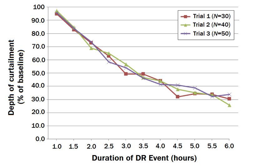
priority. system under control in the bottom-right chart of the figure.B. Continuous DR Model opposed to two objective functions in the first scenario. When
In the continuous DR scenario we try to fit a time-varying no renewable power supply is available (e.g. night time in the
random load to a random renewable supply. Unlike the classic case of solar), the z-score acceptance and rejection thresholds
DR problem where the goal is to reduce peak power con- are put into effect to ensure that no laptop dies at the expense
sumption over the duration of a DR event, the continuous of grid independence.
scenario involves matching load with supply in times of excess IV. R ESULTS FROM S IMULATION S TUDIES
and scarcity over the entire domain [0, T ] during which some
We use the same z-score function (with α = 0.25, β = 0.75,
intermittent resource is generating electricity albeit variably.
and κ = 3.0) to prioritize laptop charging schedules for both
The classic DR model assumes that all power delivered to
the classic and continuous DR simulations. A key metric we
each load originates from the grid. However, in the continuous
test in the classic DR scenario is how well our curtailment
model we assume that the intermittent supply is at the site of
algorithm performs over varying DR event durations since the
consumption with the grid available as an external resource.
available aggregate energy slack of our loads towards the end
The goal, then, is to minimize dependence on any external or
of every DR event approaches zero as the battery capacity
supplemental power supply.
of each laptop depletes (recall Figure 3). Less slack implies
less deferrability and therefore less curtailment feasibility. We
summarize our trials in Figure 5 in order to demonstrate this
relationship.
Fig. 4. Simulation run of continuous DR over two days in 15 minute time
steps.
We construct the continuous model using the same tech-
niques as the classic model with a nearly identical problem Fig. 5. Depth of curtailment as percent of baseline load with respect to DR
formulation. In this time-varying bounded knapsack algorithm, event duration.
there exists only one objective function, namely, the absolute
error of aggregate load and total supply over each time step To produce the results above, we executed a total of 330
t ∈ [0, T ] under the constraint that load does not exceed simulation runs of the classic DR model in three separate trials.
supply. The formal problem statement is We adjusted the length of the DR event from 1 to 6 hours in
st
half-hour increments and did this 10 times in each trial for
objective : minimize
X
ui Pi − P̂supply (t) a total of 110 runs per trial. In each trial we picked large
`i ∈st
values for N0 (N0 = 30, 40, and 50 for trials 1, 2, and 3,
respectively) since DR events typically occur in times of high
st
X demand. And so each curve in Figure 5 is the mean curtailment
such that ui Pi ≤ P̂supply (t) (6)
ratio over 110 runs in each of these trials. We see that the
`i ∈st
depth of curtailment over varying DR event durations provides
where ui ∈ ~ut and P̂supply (t) is the predicted supply of power a proxy for quantifying the deferrability of the loads we are
at time t. In this way, part of the performance of this supply- modeling without directly knowing the energy slack of these
following algorithm depends on the accuracy of the predictor. loads. Therefore, the deferrability of the system in this scenario
We quantify the error between load and supply as the grid varies indirectly with the length of a DR event.
dependence which is defined on a real-valued scale of [0,1] We then assess the performance of our algorithm tailored
with 0 being no dependence on external power whatsoever and to the continuous DR scenario using public solar PV data
1 being total dependence. from rooftops across 12 locations around the United States
The continuous scenario employs the same sort-and-assign for 5 days of summer (7/8/2010-7/12/2010) and 5 days of
procedure to populate the entries of ~ut by using the z-score winter (12/19/2010-12/23/2010) for a total of 120 day-location
of each laptop to prioritize them for charge scheduling in each pairs of solar power traces [14]. Each day-location corresponds
time step but with only a single objective function to fulfill as to a unique simulation run, all of which are then used tobuild performance trials based on different supply prediction V. C ONCLUSION
techniques. These results demonstrate that it is possible to leverage sen-
In these trials we wish to determine how much reliance sor/actuator networks to manage in real-time a large number
on external power supply (perhaps either in the form of of distributed battery-powered mobile devices for a classic DR
utility-provided electricity, on-site energy storage, or backup scenario in a way that could meet the curtailment objectives
generation) is needed to buffer demand as the renewable of a demand response program participant, or for a continuous
supply fluctuates. To quantify this fluctuation, we invoke the DR scenario that optimizes available variable energy resources
notion of scaled incremental mean volatility (scaled IMV) [15] like wind or solar by reducing dependence on an external
which is simply the absolute difference between the moving power grid. By examining a single category of devices ubiq-
average of the supply signal and the actual observed supply, uitous and dispersed within modern buildings and elsewhere,
averaged over the time domain of interest and scaled according we develop strategies that treat all of these devices as one
the ratio of total energy demanded over total energy supplied load in the context of an energy management system (EMS)
in that domain. The scaled IMV gives us insights into the and anticipate similar DR approaches to the plug-in electric
high-frequency fluctuations of our supply signal which could and hybrid vehicle problem. In a real-world EMS, our on-
be the result of sporadic cloud cover (in the case of solar) line algorithm could work in conjunction with a whole suite
or microbursts (in the case of wind) without bias to energy of load management controls and algorithms for buildings or
imbalances in supply and demand. microgrids.
ACKNOWLEDGEMENTS
This work is supported by the U.S. Department of Energy
(Distributed Intelligent Automated Demand Response Award
Number: DE-EE0003847) and National Science Foundation
(CPS-LoCal Grant Number: CNS-0932209). The views and
conclusions contained in this document are those of the authors
and should not be interpreted as representing the official
policies, either expressed or implied, of the U.S. Department
of Energy or National Science Foundation.
R EFERENCES
[1] D.B. Crawley, L.K. Lawrie, F.C. Winkelmann, et al., “EnergyPlus: creating a new-
generation building energy simulation program,” Energy and Buildings, Elsevier,
Vol.22, Issue 4, pp. 319-331, April 2001.
[2] Y. Lu, P. Mukka, T. Gruenwald, “Building Management System and OpenADR
Fig. 6. Semilogarithmic scatter plot of grid dependence as a function of the Integration,” Distributed Intelligent Automated Demand Response (DIADR),
scaled IMV of the supply signal for a specific day (i.e. simulation run) of Siemens Corporate Research, Nov 2010.
all three supply prediction trials compared to the unmanaged base case trial [3] X. Jiang, M.V. Ly, J. Taneja, et al., “Experiences with a High-Fidelity Wireless
without any charge scheduling algorithms applied. Building Energy Auditing Network,” SenSys ‘09, ACM, Nov 2009.
[4] D.B. Arnold, N.A Murthy, M. Sankur, et al., “DIADR Local Control Testing in a
Laboratory Environment,” A Distributed Intelligent Automated Demand Response
Buliding Management System, DOE Award Number: DE-EE0003847, University
In Figure 6 we present the results of four distinct trials of California, Berkeley, Sept 2011.
corresponding to one unmanaged base case scenario in which [5] S. Dawson-Haggerty, S. Lanzisera, J. Taneja, et al., “@scale: Insights from
a Large, Long-Lived Applicance Energy WSN,” Proceedings of the 11th
our algorithm is not applied, and three applied scenarios ACME/IEEE Conference on Information Processing in Sensor Networks, SPOTS
employing three distinct supply prediction models for per- Track (IPSN/SPOTS ‘12), April 2012.
[6] J. Taneja, D. Culler, P. Dutta, “Towards Cooperative Grids: Sensor/Actuator
formance comparison. The base case (solid black) assumes Networks for Renewables Integration.” IEEE SmartGridComm ‘10, Oct 2010.
loads obliviously consume power regardless of the renewable [7] I. Schinca, I. Amigo, “Using renewable energy to include off-grid rural schools
into the national equity project Plan Ceibal,” International Conference on
supply, in which case we do not apply any load control. In Biosciences, pp. 130-134, March 2010.
one algorithm-applied trial we use a persistence model (dotted [8] D. Soto, E. Adkins, M. Basinger, et al., “A prepaid architecture for solar electricity
delivery in rural areas,” ICTD ‘12, pp. 130-138, March 2012.
red) in which we assume that the power supply in the current [9] J. Flinn and M. Satyanarayanan, “PowerScope: A Tool for Profiling the Energy
time step will be the same in the next time step; in the next Usage of Mobile Applications,” IEEE Workshop on Mobile Computing Systems
and Applications, pp.2-10, Feb 1999.
trial we use a 1-hour moving window average (dashed green) [10] L. Zhang, B. Tiwana, Z. Qian, et al., “Accurate online power estimation and
of historical data to predict supply in the next time step; and automatic battery behavior based power model generation for smartphones,”
CODES/ISSS ‘10, pp.105-114. Oct 2010.
in the final trial we use an oracle (dash-dot blue) in which [11] A. Brooks, E. Lu, D. Reicher, et al., “Demand Dispatch: Using Real-Time Control
we know exactly how much solar will be available in every of Demand to Help Balance Generation and Load,” IEEE Power and Energy
Magazine, Vol.8, Issue 3, pp.20-29, May 2010.
time step. The average base case grid dependence of oblivious [12] J. Lee, A Varuttamaseni, F. Rahman, “Optimization of the Integrated Electric
charging is 0.561. The average grid dependencies over each Grid,” DTE Energy MPSC PHEV Pilot Project, University of Michigan, Ann
Arbor, January 2011.
algorithm trial of 0.411, 0.380, and 0.371, respectively, reflect [13] S. Studli, E. Crisostomi, et al., “AIMD-like algorithms for charging electric and
a 26.8-33.8% improvement to the base case when our sort- plug-in hybrid vehicles,” IEEE Electric Vehicle Conference, March 2012.
[14] Rooftop solar traces available from http://view2.fatspaniel.net/SSH/MainView.jsp
and-assign knapsack algorithms are applied to laptop charging [15] M. Roozbehani, M. Dahleh, S. Mitter, “Volatility of Power Grids under Real-
schedules. Time Pricing,” LIDS Report, MIT. June 2011.You can also read