Energy saving potential with smart thermostats in low-energy homes in cold climate
←
→
Page content transcription
If your browser does not render page correctly, please read the page content below
E3S Web of Conferences 172, 09009 (2020)                                                                 http://doi.org/10.1051/e3sconf/202017209009
NSB 2020

         Energy saving potential with smart thermostats in low-energy
         homes in cold climate
          Tuule Mall Kull1,*, Karl-Rihard Penu1, Martin Thalfeldt1, and Jarek Kurnitski1,2
         1Nearly   Zero Energy Buildings Research Group, Tallinn University of Technology, Ehitajate tee 5, 19086 Tallinn, Estonia
         2Department   of Civil Engineering, Rakentajanaukio 4 A, Aalto University, FI-02150 Espoo, Finland

                        Abstract. Smart home systems with smart thermostats have been used for years. Although initially mostly
                        installed for improving comfort, their energy saving potential has become a renowned topic. The main
                        potential lies in temperature reduction during the times people are not home, which can be detected by
                        positioning their phones. Even if the locating is precise, the maximum time people are away from home is
                        short in comparison to the buildings’ time constants. The gaps are shortened by the smart thermostats, which
                        start to heat up hours before occupancy to ensure comfort temperatures at arrival, and low losses through high
                        insulation and heat-recovery ventilation in new buildings, which slow down the cool-down process additional
                        to the thermal mass. Therefore, it is not clear how high the actual savings can be for smart thermostats in new
                        buildings. In this work, a smart radiator valve was installed for a radiator in a test building. Temperature
                        setback measurements were used to calibrate a simulation model in IDA ICE. A simulation analysis was
                        carried out for estimating the energy saving potential in a cold climate for different usage profiles.

       1 Introduction                                                          larger when lower temperatures are allowed during
                                                                               nighttime.
       Smart thermostats including programmable setpoints and                      In this work, the energy saving potential for a set of
       learning of heat-up time have been used for a decade                    different setpoint and internal heat profiles is estimated in
       already. Still, energy saving has not been in the top                   a energy-efficient building. The results are based on
       interests of the users [1]. However, with very energy-                  simulations on a calibrated model of room, radiator and
       efficient buildings and people’s awareness, the topic has               smart thermostat.
       become more important.
           Many smart home providers advertise energy savings
       as they locate the owners by their smartphones and switch               2 Methods
       off the heating when there is no one home [2]. When the
                                                                               The study consisted of four main parts shown in Fig. 1:
       owners approach home, the heating turns on again. This
                                                                               • Measurements in a test house,
       means that the savings heavily depend on the behavior of
                                                                               • Building model calibration in IDA ICE 4.8 SP1 [3],
       the people. It has been also analyzed how to change their
                                                                               • Simulations for energy savings of one room,
       behavior for more energy savings.
                                                                               • Simulations for energy savings in a small residential
           However, even if the people behave predictably, the
                                                                               house.
       nearly zero energy buildings cool down extremely slowly
       and therefore, the saving potential can be limited.
       Especially if the thermostat has to heat up the building for                          Measurements in a test house
       the arrival of the occupant, reducing the free-float times
       even more.
                                                                                           Calibrating the test room model
           Another restriction for the energy saving in multi-
       room dwellings is the difference in usage and setpoint                                    Calibration of physical parameters
       profiles between the rooms. When a room is not heated,
       the adjacent rooms are heated more and the overall energy                                    Calibration of controller logic
       consumption does not change much. If we use the same
       profile for the whole house, the gaps when heating is not
                                                                                         Annual simulations of the test room
       needed are shorter and the time often overlaps with solar
       gains for residential buildings. This is the period when
       heating is not often needed in the low energy buildings                     Transfer the test room to residential house for
       due to high influence of solar gains and therefore the                                whole building simulations
       savings are small. The energy savings can be clearly                    Fig. 1. Flow chart of the applied methodology

         *
             Corresponding author: tuule.kull@taltech.ee

  © The Authors, published by EDP Sciences. This is an open access article distributed under the terms of the Creative Commons Attribution License 4.0
  (http://creativecommons.org/licenses/by/4.0/).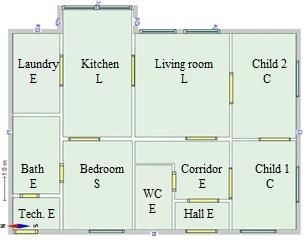
E3S Web of Conferences 172, 09009 (2020) http://doi.org/10.1051/e3sconf/202017209009
NSB 2020
2.1. Measurements
The aim of the physical experiment was to gather input
data for room and radiator model calibration at changing
setpoint (Tset) as well as to estimate how a smart home
thermostat could work. The experiment was carried out
during a 13-day period in February 2020, including 9 Fig. 3. Temperature setpoint of the smart thermostat during the
weekdays and 4 weekend days. It was performed in a test weekdays and the second weekend, during the first weekend, the
house at TalTech university campus in Tallinn, Estonia. setpoint was constantly on 21°C
The building has one floor with 100 m2 and an unheated
attic space fully open to the inner corridor. The external During the 13-day long experiment, the smart
walls and the roof are wooden frame construction, under thermostat of the radiator had a variable setpoint shown in
Fig. 3. Additional heat was generated by a 90-W internal
the concrete floor there is crawlspace. The U-values of the
constructions are the following: external walls 0.12, heat gains source, which emulated a person. During the
windows 0.75, roof and floor 0.08 W/(m2K). weekdays it turned on at 5 p.m. and off at 9 a.m. During
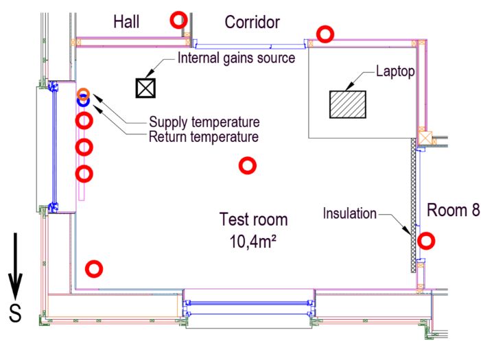
The measurements were carried out in one test room the weekends, it heated the whole 24 hours. A laptop was
shown in Fig. 2, the measurement points are shown in red on the table, emitting heat at about 13 W constantly. Both
devices were plugged into smart sockets and therefore the
circles. The room area is 10.4 m2; it has two 4-m2
dynamic emission powers are known.
windows, one toward south and the other facing west. The
air temperature (Tair) was measured in the centre and in The weather data was measured locally on the roof of
the corner of the room at 1-m height. The air temperatures the test house. Air temperature (Tout) measurements as
were also measured in the adjacent rooms. The door to test well as diffuse and global irradiation on horizontal were
room 8 in the east was insulated with 50-mm insulation available. The direct solar irradiation was calculated as
the difference of the two latter measurements. It was also
board and taped for air-tightness. The southern wall has
through-wall test ventilation units, which were also taped. converted to direct normal irradiation using the solar
The ventilation was turned off and the valves taped. elevation angles from the IDA ICE software.
The test room was heated with one floor-connected
type-11 hydraulic radiator, 1.2 m long and 0.3 m high with 2.2 Model calibration and adaption
nominal power of 263 W. The radiator was equipped with
a smart thermostat. Three temperature sensors were A simulation model of the test house was calibrated in
installed on the radiator surface. The supply and return IDA ICE 4.8 SP1. The model has been previously
temperatures (Tsup and Tret, blue and orange circle in calibrated for different experiment setups [4–6].
Fig. 2) were measured on the external surface of the Therefore, the constructions were assumed to be already
supply and return pipes between the floor and the radiator valid.
in the room. The calibration was done in two steps. Initially,
An air-to-water heat pump prepares the supply measurements from the physical experiment were used
temperature for the radiators in this test house. The set wherever possible to determine some unknown
supply temperature was an outdoor temperature parameters of the room and the radiator. Secondly, the
compensated heating curve with 45°C at -10°C, 39°C at unknown logic of the commercial smart thermostat was
0°C and 31°C at 10°C. All the other radiator circuits were emulated. The aim was to find a logic that results in
closed from the collector so the mass flow could have energy consumption as similar as possible to the measured
been measured at the mixing station. The pump at the case.
mixing station was set to a constant power mode of lowest
level possible. The distance from the mixing valve to the 2.2.1 Room and radiator calibration
measured radiator is almost 10 m.
The physical parameters in the test house, which still
needed calibrating, were all the leaks from the test room
to other rooms and outside, dirtiness of the windows and
the transparency of the trees in the park. Time constant
and the convection-radiation split of the internal gains
were also adapted.
A mathematical optimum was not needed for our
application, so the suitable parameter values were found
by trial and error of logical parameter value ranges and
noting tendencies to choose next combinations. Several
parameters were varied simultaneously and several
iterations were done before the final parameter values
were fixed.
In the calibration model, the measured weather data
Fig. 2. Test room floor plan with sensor locations (red circles),
was used. Also, air temperatures in the adjacent rooms
orange and blue circles note the location of supply and return were enforced by using ideal heaters and coolers. In the
temperature sensors test room, the input parameter was the supply
2E3S Web of Conferences 172, 09009 (2020) http://doi.org/10.1051/e3sconf/202017209009
NSB 2020
temperature. The radiator mass flow was controlled by a simultaneously two people in the living areas of 32 m2
proportional-integral (PI) controller, which attempted to (180 W / 32 m2 = 5.6 W/m2). The maximum internal gains
follow the measured return temperature. The measured from equipment was assumed to be 3 W/m2 multiplied by
mass flows, radiator surface temperatures and air the profile given in the Estonian regulation [8] and shown
temperatures in the room were used only for comparison. in Fig. 5.
The main aim was to get the average absolute integrated The helping rooms such as corridors, bathrooms,
error (AAE) between the measured and simulated air laundry rooms, etc. are called type “extra” in the
temperatures minimal, as this determines the heat losses following. These rooms had same setpoint profiles as
from the room. living areas. However, these rooms did not include
Finally, the radiator parameters were varied to get the internal gains from people, only the internal gains from
mass flows to match. equipment.
The sleeping areas are master bedrooms, which are
only used at night. The room was assumed to be used by
2.2.2 Controller estimation
two people so the maximum internal gain was assumed to
To enable simulations over the whole heating period, the be 2 x 90 W. Children’s rooms are used not only for
control of the radiator has to function without the sleeping but more extensively. Child area was assumed to
measured inputs. The supply temperature setpoint for the be for one child, so the internal heat generation maximum
heat pump is known. However, the actual temperatures was 90 W. For sleeping and children’s rooms a variation
fluctuate and decrease before reaching the radiator. So in was tested with cold temperatures allowed during sleep.
addition to the set heating curve, heating curve fit from For children, the lower temperatures were allowed from 9
measured supply temperatures was tested. p.m. to 9 a.m. In the master bedroom this results in
The thermostat controls the radiator somehow constant 18 °C setpoint profile.
dependent on the room air temperature it measures and its
setpoint. PI control is assumed. Several different 2.3.2 Benchmark
algorithms are compared where PI parameters are varied,
input air and set temperatures modified. There is no The energy saving potential of a defined case was defined
measurement point away from the radiator, so the radiator as the relative change in the net heating demand compared
surface temperature compensated air temperature is tested to the benchmark case. The benchmark case had
as the air temperature input. It is clear that after some temperature setpoint constantly at 21°C. The benchmark
learning period, the radiator introduces pre-heating to was different for each case as the internal gains of the
reach the given setpoint at given time. Therefore, the compared case were kept.
setpoint is changed so that the higher levels start earlier.
A linear change of the setpoint is also tested.
2.3 Heating period simulations
2.3.1 Input data
The saving potential of the intermittent heating was
evaluated on heating period of October 1st to April 30th.
Estonian Test Reference Year (TRY) was used for the
weather data [7]. Heat recovery ventilation with 80 %
efficiency was added to all cases as comparison. The
supply air temperature was fixed to 17 °C with balanced
air flows of 0.42 l/sm2. If the ventilation supply
temperature were higher than the lower level, the savings
would have been less.
The internal gains and temperature setpoints were
varied to emulate four different room usage types: living Fig. 4. Defined usage profiles of the different rooms
areas, sleeping areas, children’s rooms and helping rooms.
The usage profiles by hour of the day are shown in Fig.
4.The shown on-off signals represent both when the
internal gains from people and the temperature setpoints.
The internal gains lower level was zero and the maximum
level was defined separately for each profile type and is
defined below. The lower setpoint was 18 °C and the
higher 21 °C.
Living areas such as living rooms and kitchens are
used in the mornings and evenings. In the living areas, the
maximum internal gain from people was fixed to 5.3 Fig. 5. Equipment usage profile in livng and extra areas
W/m2 as in the used residential house there are
3E3S Web of Conferences 172, 09009 (2020) http://doi.org/10.1051/e3sconf/202017209009
NSB 2020
2.3.2 Simulation tests So secondly, a whole house with a mix of different
profiles was simulated. The house is essentially the
First, the saving potential was estimated in the test room calibrated test building but the floor plan is adjusted to a
with adjacent rooms kept at 21 °C. It is clear that the more typical residential building. An example of a 100 m2
adjacent rooms heat the test room in this case. So the net one-family house was used, which has been also applied
heating demand was calculated adding up the radiator heat in Estonian guidelines for nearly zero energy buildings
emission and heat fluxes through internal constructions and scientific publications before [9, 10]. The room areas
and leaks. were changed from the original to include the test room in
In reality, rooms of different usage are next to each the original size for comparisons. Also the orientation
other. So some of the time one room cools down, the remains the one of the test house and the windows as well.
adjacent room heats it. Therefore, the resulting saving Only two windows from the northern facade were shifted
potential in a whole building would be very different than to the eastern facade. The resulting floor plan is shown in
the savings of different room types added up. Fig. 6. The capital letters note the profile types used in
these rooms: living L, sleeping S, children C, and extra E.
By area the profile types are divided as follows: 34%
living, 11% sleeping, 23% children, 31% extra. To
compare different profiles both simulated separately and
in the mix of profiles, for some cases the bedroom and
room child1 were exchanged in their function but not in
the areas as the difference in areas is just 1 m2.
3 Results
3.1 Calibration precision
The parameter values, which resulted in the most accurate
air temperatures and mass flows, compared to the
measurements, are shown in Table 1. The default IDA
ICE water radiator model was changed to the dynamic
Fig. 6. The floor plan of the simulated residential house, the radiator with mass modelled to get dynamically better
letters note the usage type applied to the rooms
results. All radiator parameters that were given by its
Table 1. The varied parameters and their values for the producer were defined as designed.
calibrated model As the supply and return temperatures were measured
on the pipes, the temperature dropped to room
Parameter Value temperature when there was no mass flow. Therefore, for
Dirtiness of windows more exact simulation the radiator was turned off while
40 %
Solar
gains
(g-value reduction) the supply temperatures were below 22 °C. Otherwise, the
mass flow was controlled by a PI controller, which
Transparency of the park 0.3 tracked the return temperature. Optimizing its control
Internal gains time constant 600 s parameters did not improve the results.
Internal
gains
The optimal solution reached AAE of 0.25 K. The
Internal gains model was then further used to estimate the control. In this
0.8
convection-radiation split process, the supply temperature was chosen first. One of
Leak to outside 0.8 l/s
the heating curves was the setpoint given to the heat
pump. The second was the linear model fitted from the
Air flows
Leak to attic 1.2 l/s measured data at times with significant mass flow (at least
0.015 kg/s). The latter showed AAE of 0.23 K while the
Leak area to Corridor 0.1 m2
first had AAE of 0.37 K. What is more important here, the
Leak area to Room 8 0.005 m2 total radiator heat output during the experiment was 2%
higher than the calibrated case for the fitted supply
Heat transfer between Only temperature and 12.6 % higher for the setpoint curve.
radiator and the wall radiative
Radiator heat emission
Therefore, the fit temperature curve was further applied.
Heat transfer coefficient The model was:
between liquid and 100 W/K
the radiator surface = −0.6065 ∙ + 35.182 [℃] (1)
Heat transfer coefficient
40 W/K The mass flows showed that after some initial
between surface and ambient
learning, the smart thermostat started to heat before the
Minimum mass flow 1e-4 kg/s setpoint was actually raised. For the weekday morning
high temperature period, it started around 1 to 1.5 hours
Maximum mass flow 0.02 kg/s
early, and for the evening peak around 2 to 3 hours early.
4E3S Web of Conferences 172, 09009 (2020) http://doi.org/10.1051/e3sconf/202017209009
NSB 2020
However, the times clearly varied from one day to
another. The optimal solution was to use a linearly
increasing setpoint, which started to raise 1 h early for the
morning, and 3 hours early for the evening peak.
The air temperature of the controller also seemed to be
something else than measured elsewhere in the room as
the controller almost never reached the setpoint. We
assumed that at the thermostat the temperature had been
higher. We found a correction factor dependent on the
radiator surface temperature. Applying the suitable
correction factor to the air temperature, we got an
indication what temperature the thermostat could have
measured:
_ = ( − 20)/20 + [℃] (2)
where Tsurf is the radiator surface temperature 30 s
before. Therefore, at 40 °C radiator surface temperature,
a 1 K higher air temperature would be measured, and
therefore in the center of the room, the temperature would
only reach 20 °C instead of 21 °C. However, as both the
constant setpoint and variable setpoint cases would
behave the same, the setpoints were kept as defined
previously.
Finally, the calibrated control model had AAE of 0.27
K, the radiator heat output had increased by 4.4 % from
the initial calibration. However, as the heat pump had not
reached the set temperatures at the end of the experiment,
just changing the supply temperature to the fitted model
had increased the heat output by 2 %. The change from
there was just 2.4 %.
The air temperatures, mass flows, supply, return and
radiator surface temperatures for the measured, calibrated
and the calibrated control cases are shown in Fig. 7. We
can see that the air temperatures match very well along all
the cases but never drop lower than 19 °C. For the
calibrated case, also the mass flows and supply and return
temperatures fit well to the measurements. For the mass
flows, the times when the radiator is turned off, there is
some flow measured in the mixing station due to the
bypass. This can be omitted for the radiator.
For the calibrated control, mass flows are fluctuating
much less than measured. It was attempted to change this
situation by varying PI control parameters but
unsuccessfully. Due to higher average flows, the return
temperature was lower.
The simulated radiator surface temperatures are not
fitting that well to the measurements. As in IDA ICE, the
convective heat emission of the radiator does not
influence the surface temperature, it is clear that these are
not exactly the same and do not have to match. The
surface temperatures between the calibration and
calibrated control match.
Although the total heat emission during the
experiment period is very similar between the calibration
and calibrated control, the dynamic heat output profile of
the calibrated control fluctuates lot less. There are also
some imprecision at heating starting and stopping times.
Fig. 7. The calibrated base and calibrated control results
compared to the measurements
5E3S Web of Conferences 172, 09009 (2020) http://doi.org/10.1051/e3sconf/202017209009
NSB 2020
3.2 Energy saving potential
The energy saving potential results are shown in Fig. 8.
The room-based results on the left show that for the
different profiles the energy saving potential ranged from
7 to 29 % for the calibrated control case with no
ventilation. When ventilation was added, the savings were
1 to 4 % higher. The whole house profile mix (MIX) cases
showed lot lower savings potential, 8 to 11 % with
ventilation. Sleeping cold and child cold are the
corresponding profile types with night setbacks allowed.
It is clear that the energy saving potential is closely
related to the time that lower setpoints are allowed. As the
smart thermostat applied some pre-heating, the heat-up
process was included in the heating period simulations as
well. For most cases, the higher temperature level was
kept for a longer period of time than 3 hours, so the 3-hour
Fig. 8. Energy saving potential for the different profiles with pre-heating was applied. Only in the case of living areas
boundaries at 21°C (room) or in the mix of different profiles morning peak, the one-hour heat-up was used. The
(house) with and without heat recovery ventilation percentage of the week spent at different setpoint levels
or in the pre-heating process are shown in Fig. 9 for all
profiles.
Plotted against the percentage of time at setpoint 18
°C (blue columns in Fig. 9), the energy saving potential is
visualised in Fig. 10. The room-based results linearly
depend on this time. The cases with ventilation depend on
it with a steeper rise than the cases without ventilation. As
an example, the results for the room Child 1 in the house
with a mix of profiles is separated. It can be seen, that the
energy saving potential has decreased compared to the
case its boundaries are constantly at 21 °C without any
additional internal gains raising the temperatures (black
arrows indicate the change). The decrease is up to 3 % for
this and the sleeping room.
The time at lowest setpoint for the house results is
Fig. 9. The share of time the setpoint is high, low, or in-between calculated as the area-weighted average of the profiles.
for the different setpoints The house results have clearly lower energy saving
potential than the rooms separately. The cases would still
lie lower than the linear lines even if the lowest time
percentage over all the profiles in the mix would be used.
In modern homes, air temperature setpoint is often
higher than standard 21 °C. To observe its effect on
energy saving, two additional cases of the house were
simulated. The constant reference situation was raised by
2 °C to 23 °C, all the variable profiles were raised by 2 °C
resulting in profiles with lower level at 20 °C and higher
at 23 °C. Due to higher gradient to outdoor, the losses
would be higher at higher temperatures. However, the
heating would have to use more energy to compensate for
this. In the 20/23 °C profile case for the MIX with
ventilation, energy saving was 7.6 kWh/m2, which is 6 %
of the constant 23 °C. The relative difference is similar to
the 8 % saving shown for 18/21 °C above. However, in
the 18/21 °C case, the absolute energy saving was 2.2
kWh/m2. Therefore, the absolute saving at higher
temperature profile is clearly higher and the relative
saving is a bit lower. The lower relative difference could
be caused by the fact that 3 °C setback in the profile makes
up smaller proportion of the indoor to outdoor
temperature gradient in the higher profile case.
Fig. 10. Energy saving potential dependent on the percent of
time the profile has setpoint of 18 °C
6E3S Web of Conferences 172, 09009 (2020) http://doi.org/10.1051/e3sconf/202017209009
NSB 2020
4 Discussion References
It was possible to calibrate the measured data very 1. D. Malekpour Koupaei, T. Song, K. S. Cetin, and J.
precisely when the radiator supply and return Im, Build. Environ., vol. 170, p. 106603, 2020.
temperatures were known. It was a bigger challenge to 2. U. Ayr et al., IOP Conf. Ser. Mater. Sci. Eng., vol.
find a control algorithm that would explain what the smart 609, no. 6, 2019.
thermostat did. However, with the found solution the 3. EQUA, “IDA Indoor Climate and Energy (IDA
energy consumption and air temperature were closely ICE, version 4.8 SP1, Expert edition).” 2019.
matched to the measurements. 4. M. Maivel, A. Ferrantelli, and J. Kurnitski, Energy
As the radiator was measuring lower temperature for Build., vol. 166, pp. 220–228, 2018.
air than it was in the centre of the room, the centre almost 5. T. M. Kull, M. Thalfeldt, and J. Kurnitski, J. Phys.
never reached the setpoint. Usually, a temperature Conf. Ser., vol. 1343, no. 1, 2019.
setpoint shift is carried out in such a situation. However, 6. K. V. Võsa, A. Ferrantelli, and J. Kurnitski, E3S
here it was not done as the comparison was relative and Web Conf., vol. 111, no. 201 9, 2019.
the shift should have been applied both to the constant and 7. T. Kalamees and J. Kurnitski, Proc. Est. Acad. Sci.
the variable setpoint. Eng., vol. 12, no. 1, pp. 40–58, 2006.
Not reaching the setpoint temperatures could also be 8. “Estonian Regulation No 58” Ministry of
explained by the very low mass flows in the heating Economic Affairs and Communications, 2015.
system. The system should also be calibrated in a normal 9. R. Simson, E. Arumägi, K. Kuusk, and J. Kurnitski,
functioning case with several radiators to clarify whether E3S Web Conf., vol. 111, no. 201 9, 2019.
the response to changing the setpoints is same in principle. 10. Tallinn University of Technology, 2017. [Online].
The variable profiles really have a huge impact, our Available: https://kredex.ee/sites/default/files/2019-
study shows. However, to get an overview, what the real 03/Liginullenergia_eluhooned_Vaikemaja_juhend.
extents are, a large variety of different profiles should be pdf. [Accessed: 03-Apr-2020].
simulated. A stochastic approach should be applied too
but then the logic of the controller has to be known. In this
work, a black-box model of the controller was calibrated
but these models would vary for different products. For
determining the pre-heating times, the pre-heating time
was set to constant in most cases. A smart controller could
work better than just a fixed period of pre-heating.
Moreover, the internal gains are always full loads in this
work, but in future works, partial loads should be included
as well. In addition to different profiles and gains, the
building U-values and heat capacity should be varied as
well.
5 Conclusions
The aim of this work was to determine energy saving
potential of different usage and setpoint profiles in
residential low energy building in a cold climate. It was
found that the energy saving potential for the tested
profiles ranged from 7 to 33 %. However, when the same
profiles were mixed up into the rooms of a single-family
house, the energy saving potential was decreased to 8 %
saving. In future works, the analysis should be replicated
with several different smart thermostats on a variety of
realistic buildings with different heat loss and capacity.
This research was supported by the Estonian Centre of
Excellence in Zero Energy and Resource Efficient Smart
Buildings and Districts, ZEBE (grant No. 2014-2020.4.01.15-
0016) and the programme Mobilitas Pluss (Grant No 2014-
2020.4.01.16-0024, MOBTP88) funded by the European
Regional Development Fund, by the Estonian Research Council
(grant No. PSG409) and by the European Commission through
the H2020 project Finest Twins (grant No. 856602). We would
also like to thank Eesti Energia AS for supplying the thermostats
and smart sockets.
7You can also read