Experiment Photometry and Spectroscopy - Advanced Labwork in Astronomy and Astrophysics - Uni Tübingen
←
→
Page content transcription
If your browser does not render page correctly, please read the page content below
Advanced Labwork
  in Astronomy and Astrophysics

       Experiment
Photometry and Spectroscopy

       Thomas Rauch & Lisa Löbling
    Kepler Center for Astro and Particle Physics
     Institute for Astronomy and Astrophysics
                        Sand 1
                   72076 Tübingen

                  July 23rd , 2019

  http://www.uni-tuebingen.de/de/4203
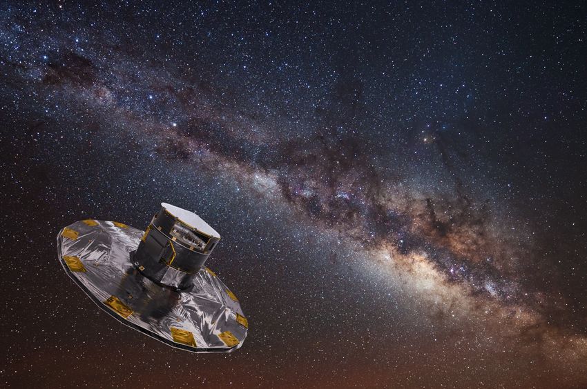
The German version of this experiment manual was created by Thorsten Nagel in the years 2004
to 2008 based on earlier manuals for a CCD-camera experiment and experimental physics lab-
work by Jörn Wilms, Stefan Dreizler, Ralf Geckeler, and Martin Bässgen, comments of Jochen
L. Deetjen, and the scientific work of Margit Haberreiter1 . The manual had been maintained
by Cornelia Heinitz from 2015 to 2017. Since then, Thomas Rauch2 und Lisa Löbling3 are
responsible.

Image on coverpage: More than four million stars within five thousand light-years from the Sun
are plotted using information about their brightness, color and distance from the second data
release from ESA’s Gaia satellite.
(http://sci.esa.int/gaia/60198-gaia-hertzsprung-russell-diagram)
  1 http://astro.uni-tuebingen.de/publications/diplom/margit-zula.ps.gz
  2 rauch@astro.uni-tuebingen.de
  3 loebling@astro.uni-tuebingen.de
Contents
1   Preface                                                                                                                      1

2   Introduction                                                                                                                 1
    2.1 Coordinate systems . . . . . . . . . . . . . . . .      .   .   .   .   .   .   .   .   .   .   .   .   .   .   .   .    1
    2.2 Telescopes . . . . . . . . . . . . . . . . . . . . .    .   .   .   .   .   .   .   .   .   .   .   .   .   .   .   .    3
         2.2.1 Aperture ratio . . . . . . . . . . . . . . .     .   .   .   .   .   .   .   .   .   .   .   .   .   .   .   .    3
         2.2.2 The resolving power . . . . . . . . . . .        .   .   .   .   .   .   .   .   .   .   .   .   .   .   .   .    4
         2.2.3 Refractors . . . . . . . . . . . . . . . . .     .   .   .   .   .   .   .   .   .   .   .   .   .   .   .   .    5
         2.2.4 Reflectors . . . . . . . . . . . . . . . . .     .   .   .   .   .   .   .   .   .   .   .   .   .   .   .   .    6
         2.2.5 Telescope mountings . . . . . . . . . . .        .   .   .   .   .   .   .   .   .   .   .   .   .   .   .   .    9
         2.2.6 Active and adaptive optics . . . . . . . .       .   .   .   .   .   .   .   .   .   .   .   .   .   .   .   .   10
    2.3 Image detectors . . . . . . . . . . . . . . . . . .     .   .   .   .   .   .   .   .   .   .   .   .   .   .   .   .   12
         2.3.1 Basic principles of CCDs . . . . . . . . .       .   .   .   .   .   .   .   .   .   .   .   .   .   .   .   .   13
         2.3.2 CCDs in astronomy . . . . . . . . . . . .        .   .   .   .   .   .   .   .   .   .   .   .   .   .   .   .   15
    2.4 Spectroscopy . . . . . . . . . . . . . . . . . . .      .   .   .   .   .   .   .   .   .   .   .   .   .   .   .   .   16
         2.4.1 Diffraction theory of a grating . . . . . .      .   .   .   .   .   .   .   .   .   .   .   .   .   .   .   .   17
         2.4.2 Dispersion . . . . . . . . . . . . . . . .       .   .   .   .   .   .   .   .   .   .   .   .   .   .   .   .   19
         2.4.3 Resolving power . . . . . . . . . . . . .        .   .   .   .   .   .   .   .   .   .   .   .   .   .   .   .   19
    2.5 Radiation theory . . . . . . . . . . . . . . . . . .    .   .   .   .   .   .   .   .   .   .   .   .   .   .   .   .   20
    2.6 Radiation intensity and radiation flux . . . . . . .    .   .   .   .   .   .   .   .   .   .   .   .   .   .   .   .   20
         2.6.1 Radiation in thermodynamic equilibrium           .   .   .   .   .   .   .   .   .   .   .   .   .   .   .   .   21
         2.6.2 Effective temperature and luminosity . .         .   .   .   .   .   .   .   .   .   .   .   .   .   .   .   .   22
         2.6.3 Magnitude and color . . . . . . . . . . .        .   .   .   .   .   .   .   .   .   .   .   .   .   .   .   .   22
    2.7 Color-magnitude diagram . . . . . . . . . . . . .       .   .   .   .   .   .   .   .   .   .   .   .   .   .   .   .   23
    2.8 Spectral classification . . . . . . . . . . . . . . .   .   .   .   .   .   .   .   .   .   .   .   .   .   .   .   .   23

3   Experimental setup                                                                                                          27
    3.1 80cm reflector of the IAAT . . . . . . . . . . . . . . . . . . . . . . . . . . . .                                      27
    3.2 10 C grating spectrograph . . . . . . . . . . . . . . . . . . . . . . . . . . . . .                                     27
    3.3 CCD cameras STL 1001E and HX916 . . . . . . . . . . . . . . . . . . . . . .                                             31

4   Experimental procedure                                                                                                      32
    4.1 Preparation . . . . . . . . . . . . . . . . . . . . . . . . . . . . . . . . . . . .                                     32
    4.2 Stellar spectroscopy . . . . . . . . . . . . . . . . . . . . . . . . . . . . . . . .                                    34
    4.3 Photometry of a stellar cluster . . . . . . . . . . . . . . . . . . . . . . . . . .                                     41

5   Literatur                                                                                                                   43

A Tentative objects for observation                                                                                             44

B Wavelength calibration                                                                                                        45

C Prominent lines in stellar spectra.                                                                                           46

D Structure of the protocol                                                                                                     49

                                                I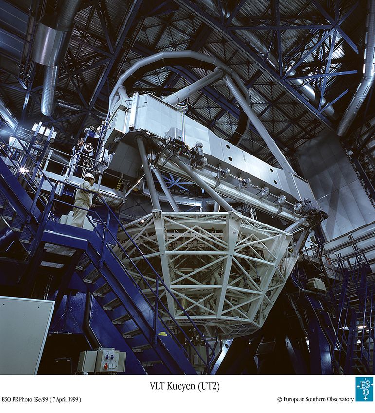
List of Figures
  1    Celestial sphere with coordinates. . . . . . . . . . . . . . . . . . .      .   .   .   .   .   .    2
  2    Derivation of the reproduction scale. . . . . . . . . . . . . . . . . .     .   .   .   .   .   .    3
  3    Function J1 (2m)/m. . . . . . . . . . . . . . . . . . . . . . . . . . .     .   .   .   .   .   .    4
  4    Diffraction image for two point sources of same brightness. . . . . .       .   .   .   .   .   .    5
  5    Optical path of the Newtonian telescope. . . . . . . . . . . . . . . .      .   .   .   .   .   .    6
  6    Mirror construction of a 8 m VLT unit. . . . . . . . . . . . . . . . .      .   .   .   .   .   .    7
  7    Main mirror of the 10 m Keck I telescope. . . . . . . . . . . . . . .       .   .   .   .   .   .    8
  8    Parallactic and azimuthal mountings. . . . . . . . . . . . . . . . . .      .   .   .   .   .   .    8
  9    Technical realization of the parallactic mounting. . . . . . . . . . .      .   .   .   .   .   .   10
  10   8 m VLT telescope of ESO in Chile. . . . . . . . . . . . . . . . . .        .   .   .   .   .   .   11
  11   Location of the Very Large Telescope. . . . . . . . . . . . . . . . .       .   .   .   .   .   .   12
  12   Principles of active and adaptive optics. . . . . . . . . . . . . . . .     .   .   .   .   .   .   12
  13   Mirror mounting of an 8 m VLT telescope. . . . . . . . . . . . . . .        .   .   .   .   .   .   13
  14   Scheme and principle of the read-out method of a three-phase CCD.           .   .   .   .   .   .   14
  15   Comparison of astrophysical detectors. . . . . . . . . . . . . . . . .      .   .   .   .   .   .   15
  16   Artist’s impression of Gaia mapping the stars of the Milky Way. . .         .   .   .   .   .   .   16
  17   Diffraction geometry at the double slit. . . . . . . . . . . . . . . . .    .   .   .   .   .   .   17
  18   Grating diffraction. . . . . . . . . . . . . . . . . . . . . . . . . . .    .   .   .   .   .   .   18
  19   Light path on a blaze grating. . . . . . . . . . . . . . . . . . . . . .    .   .   .   .   .   .   18
  20   Grating blazed to 1st order. . . . . . . . . . . . . . . . . . . . . . .    .   .   .   .   .   .   19
  21   Definition of intensity. . . . . . . . . . . . . . . . . . . . . . . . .    .   .   .   .   .   .   20
  22   Mean intensity of a stellar disc. . . . . . . . . . . . . . . . . . . . .   .   .   .   .   .   .   21
  23   Planck function, Wien’s law of displacement. . . . . . . . . . . . .        .   .   .   .   .   .   22
  24   Filter functions of the Johnson system. . . . . . . . . . . . . . . . .     .   .   .   .   .   .   23
  25   Color-magnitude diagram. . . . . . . . . . . . . . . . . . . . . . .        .   .   .   .   .   .   24
  26   Schematic HRD with luminosity classes. . . . . . . . . . . . . . . .        .   .   .   .   .   .   25
  27   Spectral classification. . . . . . . . . . . . . . . . . . . . . . . . .    .   .   .   .   .   .   25
  28   Temperature dependency of line strengths of different elements. . .         .   .   .   .   .   .   26
  29   IAAT 80 cm reflector. . . . . . . . . . . . . . . . . . . . . . . . . .     .   .   .   .   .   .   27
  30   Layout of the 10 C spectrograph. . . . . . . . . . . . . . . . . . . .      .   .   .   .   .   .   28
  31   Hg/Ne calibration spectrum. . . . . . . . . . . . . . . . . . . . . .       .   .   .   .   .   .   30

                                              II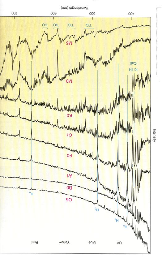
List of Tables
  1   Band gaps of different semi-conductor materials. . . . .       .   .   .   .   .   .   .   .   .   .   .   .   13
  2   Technical data of the Tübingen 80 cm reflector. . . . . .      .   .   .   .   .   .   .   .   .   .   .   .   28
  3   Technical data of the 10 C grating spectrograph. . . . . .     .   .   .   .   .   .   .   .   .   .   .   .   29
  4   Technical data of the STL-1001E camera. . . . . . . . .        .   .   .   .   .   .   .   .   .   .   .   .   31
  5   Technical data of the HX916 camera. . . . . . . . . . . .      .   .   .   .   .   .   .   .   .   .   .   .   31
  6   Filters of the STL-1001E camera at the IAAT. . . . . . .       .   .   .   .   .   .   .   .   .   .   .   .   42
  7   Object list. . . . . . . . . . . . . . . . . . . . . . . . .   .   .   .   .   .   .   .   .   .   .   .   .   44
  8   Laboratory wavelengths for Hg and Ne calibration lamps.        .   .   .   .   .   .   .   .   .   .   .   .   45

                                            III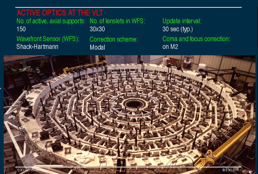
1      Preface
The experiment “Photometry and Spectroscopy” gives insight to methods of observation and
reduction of astronomical data. Especially, the technological and physical basics are in focus. In
addition to an understanding of the instruments, the practical application as well as the scientific
motivation, the underlying physics of the application examples are a key factor.
    Astronomical knowledge at the level of the introductory lecture is a prerequisite for the ex-
ecution of the experiment. Experience in handling computers is beneficial, but by no means
necessary. In this manual, we have compiled all necessary information to carry out the experi-
ment.
    The program commands for controlling the camera and the used software are all listed, but
you are not expected to cope with it without further instruction on site. In astronomy, it is still
necessary to use units that are not from the SI system. Prominent examples are the Ångström
as wavelength unit or the day as time unit. Follow this practice, please do not feel discouraged
by unfamiliar units . . .

       To simplify the experiment preparation, some easy exercises are given in this manual
      that have to be solved before the observations. Their solution is part of the protocol.
      This extended prepation is compensated by the shorted post-experiment work.

2      Introduction
In contrast to other natural sciences, astronomy is purely empirical. It is impossible for an
astronomer to manipulate the objects of their investigations under controlled conditions or to
experiment with them. The only available information is the observed radiation. The art of
astronomy is to evaluate its information.
    This observed radiation is often weak with fluxes of 10−29 W cm−2 s−1 (= 1 mJy [milli Jan-
sky], astronomical unit for flux) in the optical wavelength range or a few photons per cm2 and
s in the X-ray4 .
    Ground-based observations are hampered by the Earth’s atmosphere that the observed ra-
diation has to pass through. In addition, Earth is no fixed platform but rotates, etc. . . . The
urge to observe fainter objects leads to the development of bigger telescopes and more sensitive
detectors in the 20th century. In this manual, we will introduce you to the basics of these – as
detailed as it is necessary for the experiment. We will start with astronomical telescopes before
we explain detectors for electromagnetic radiation.

2.1         Coordinate systems
To locate astronomical objects, the definition of a coordinate system is required. It has to be
independent from observation site and time. Since, in general, we have very large distances
in astronomy (besides from objects in the Solar system), we can define a coordinate system
on an infinitely large celestial sphere and, thus, reduce it to two coordinates. Their changes
due to daily or yearly rotation of Earth is insignificantly small because the objects’ distances
are much smaller than Earth’s orbital radius (the next star, Proxima Centauri, has a distance of
about 270 000 times this radius).
    Since the Earth’s rotation axis is almost fixed in space, a projection of the equatorial system
on the celestial sphere is a well suited location and time independent reference frame. The
    4 For   cosmic radiation, particles per km2 and year is a common unit – the detection limit is about
10−2 particles  km−2 a−1 . . .

                                                     1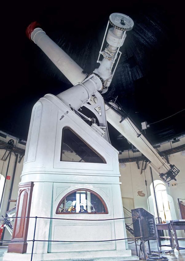
Figure 1: Celestial sphere with
                                                             coordinates.
                                                             From:       http://star-www.
                                                             st-and.ac.uk/~fv/
                                                             webnotes/chapter4.htm.

intersection line between celestial sphere and equatorial plane is a great circle that is named
celestial equator. The extension of the Earth’s rotation axis defines the celestial poles (Fig. 1).
The object’s angular distance from the equatorial plane is independent from Earth’s rotation.
This angle is measured on a great circle going through both celestial poles and the object,
the so-called hour circle. It is named declination δ (or DEC). Measured from the equatorial
plane, positive and negative angles indicate objects on the northern and southern hemisphere,
respectively. The second coordinate is measured counterclockwise on the celestial equator.
This needs a reference point that is independent from Earth’s rotation. Its selection is optional,
however, it makes sense to use one with a special significance. The projected solar orbit, the
ecliptic, meets the celestial equator at the equinoxes. The spring equinox is the reference point.
Formerly, it was located in the constellation Aries and is, thus, named First Point of Aries (ϒ).
This second coordinate is named right ascension α (or R.A.).
    The Earth’s rotation axis precession changes the coordinates. For a precise catalogue, the
indication of the time when the spring equinox was defined is necessary, the so-called epoch,
e.g., B1950 or J2000. There are other effects that affect the coordinates but this is out of the
focus of this manual.

      Exercise 1: Compile the J2000 coordinates (R.A., DEC) of the objects from the
      list (Tab. 7), e.g., from the SIMBAD data base (http://simbad.u-strasbg.fr/
      simbad).

                                                2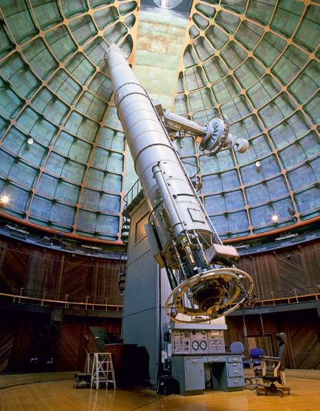
Figure 2: Derivation of the reproduction scale.

   Oh you knowing pipe, more precious                          O du vielwissendes Rohr, kostbarer
   than any scepter! Who holds you in                         als jedes Szepter! Wer dich in seiner
   his right, if he is not set for king, not                  Rechten hält, ist er nicht zum König,
   for the lord over the works of God!                              nicht zum Herrn über die Werke
                                                                                    Gottes gesetzt!
                                                                                  Johannes Kepler
                                                                                   Dioptrice, 1611

2.2     Telescopes
From the factors described in the introduction, the following requirements for astronomical
telescopes can be derived. They must have
    • a high light efficiency,
    • a high resolving power, and
    • a high image quality.
Two different classes of telescopes exist to achieve these. These are refractors, where the image
is obtained with lenses, and reflectors, where a combination of spherical and parabolic mirrors
does the same.

2.2.1   Aperture ratio
Both telescope types have in common, that an astronomical object in infinite distance is pro-
jected on the focal plane with a lens or concave mirror with a diameter D and a focal length
 f . Figure 2 shows as an example the optical path in a simple reflector. The ratio D/ f is called
aperture ratio of the optical system. For a classical picture camera, the inverse of the aper-
ture ratio f /D, is known as f-number. From Figure 2, the image size a of an object in infinite
distance with an angular diameter of ω, can be determined.

                                         a = 0.0175 ω f   ,                                     (1)

where ω is measured in degrees. A telescope with a receiving surface ∼ D2 concentrates the
energy of an extended object on an area ∼ f 2 . The ratio defines the effective luminosity
                                                       2
                                                        D
                               effective luminosity ∝            .                         (2)
                                                        f
    The effective luminosity of extended objects depends only on the aperture ratio only, e.g.,
in the case of a camera on the “f-number”. For a point source, it is

                                                 3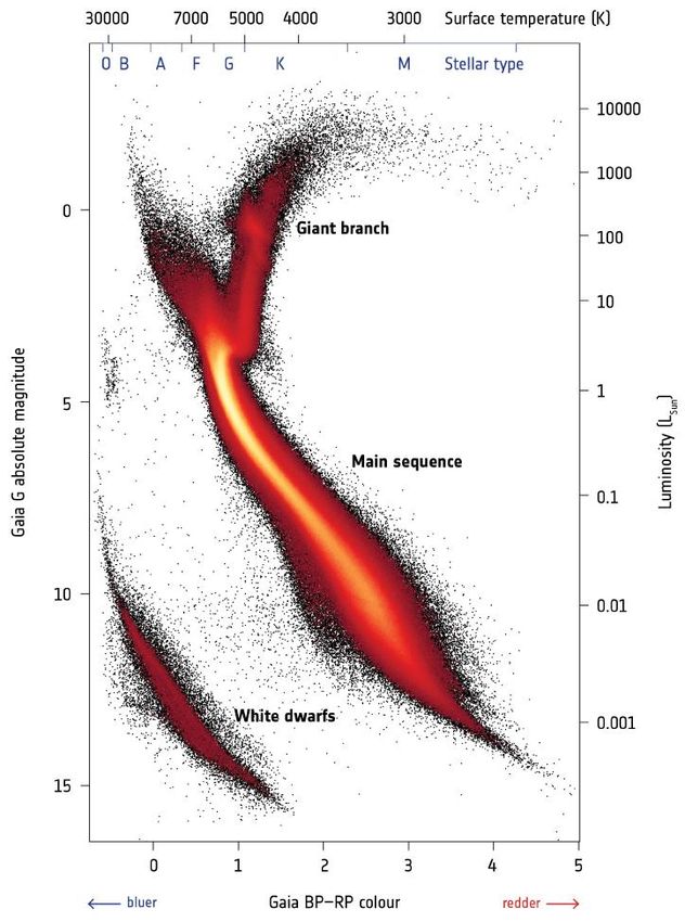
Figure 3: Function J1 (2m)/m.
           1.0                                                             The square describes the in-
                                                                           tensity distribution of a circu-
           0.8
                                                                           lar aperture. (Eq. 4).
           0.6
J1(2m)/m

           0.4

           0.2

           0.0
           -0.2
               0            2                   4                  6
                                     m

                                     effective luminosity ∝ D2         .                               (3)
   Most astronomical objects a very far, i.e., point sources and, thus, astronomical telescopes
should have large diameters to collect as much light as possible.

2.2.2        The resolving power
The resolving power of astronomical telescopes is limited by the diffraction of the coherent
light emitted by astronomical objects. For the intensity distribution I(θ) of a circular aperture
with radius r, the diffraction theory gives for an angular distance θ (z.B. Born & Wolf, 1980;
Kitchin, 1984)

                                                π2 r4
                                         Iθ ∝         (J1 (2m))2                                       (4)
                                                 m2
where
                                                πr sin θ
                                             m=                                             (5)
                                                    λ
J1 (2m) is the first order Bessel function of first kind. In Figure 3, J1 (2m)/m is shown. The
intensity is zero in concentric rings with radius

                                  1.220 λ      2.233 λ    3.238 λ
                                θ≈         ,           ,           ,...                        (6)
                                      d           d           d
where d = 2r is the diameter of the diffraction disc. The innermost is named Airy disc, after
the Royal Astronomer George B. Airy, who derived Eq. 4 for the first time. Figure 4 illustrates
Airy discs for two point sources of the same brightness with a distance of 4.46 λ/d. The image
of an astronomical object taken with a telescope appears as an extended disc of radius 1.22 λ/d,
surrounded by diffraction rings.
    To characterize the resolution of a telescope, usually the criterion invented by Lord Rayleigh
is used. It says, that two equally bright objects can be resolved, when the intensity maximum
of the diffraction pattern of the first object coincides with the first intensity minimum of the
diffraction pattern of the second. Thus, the resolution α is

                                                     1.220 λ
                                          α[rad] =           .                                         (7)
                                                        d

                                                    4
Figure 4: Diffraction image for two point
sources of same brightness with a distance
of 4.46 λ/d from a circular aperture, shown
with negative intensity like common in as-
tronomy (more dark means brighter).
Exercise 2: Calculate the resolution (in arc seconds) of a telescope with a diameter of
d = 0.6 m at a wavelength of 6562 Å.
The derivation above shows that the Rayleigh criterion is only a coarse approximation for the
resolving power of a telescope. The achievable diffraction-limited resolving power is strongly
dependent on the intensity ratio of the objects, i.e., a faint object is harder to detect in the vicinity
of a bright one. Additionally, in case of ground-based observations, the Earth’s atmosphere is
the limiting factor (Sect. 2.2.6). Thus, for practical work α ≈ λ/d is a sufficient approximation.
2.2.3 Refractors
The scientific use of telescopes started with Galileo Galilei’s demonstration how they “bring
closer” distant objects on the Campanile de San Marco in Venice on August 21, 1609. Galilei
had heard rumors about the discovery of a Dutch glas maker, namely Hans Lippershey, and
build an own telecope by a combination of a converging and a diverging lens. In negation of
the real creatorship, this telescope type is called “Galilean telescope”. Thanks to this subtle
marketing, Galilei got his salary doubled.
An alternative to the Galilean telescope was proposed by Johannes Kepler in his Dioptrice
(1611), a combination of two converging lenses – the so-called Keplerian telescope. In con-
trast to the Galilean, it has a real focal plane, i.e., it can be used for quantitative astronomical
measurements and not only for observations.
Although refractors are used for some purposes, e.g., binoculars, they are not used as astro-
nomical instruments anymore. The main reason is, that the maximum possible diameter of a
refractor is about 1 m, i.e., at a relatively small light collection area. Larger lenses are difficult
to produce without air inclusions and, due to their high weight, very difficult to stabilize. A
change in the pointing direction leads to a strong deformation of the lenses, in contrast to a
mirror that can be properly supported. Expressed less academic here – “strong deformation”
means nothing else but “disruption”. In addition, the construction length of a refractor is equal
to its focal length, leading to strong flexure of the instrument. Finally has to be considered,
that the refractive index of glas depends on the wavelength and causes image errors (chromatic
aberration).
Therefore, reflectors are the dominating telescope type since the middle of the 20th cen-
tury. Those refractors that still exist in some observatories like in Tübingen are only museum
5Figure 5: Optical path of the Newtonian telescope. (Newton, 1730, Fig. 29).
pieces and not used for actual scientific projects5 . The only exception are special purposes of
astrometry, i.e., the measurement of stellar positions, where refractors with typical diameters
< 30 cm are used as so-called Meridian circles. These instruments have also been more and
more replaced since 1985, e.g., by the European satellites Hipparcos or Gaia.
A very nice review about the historical competition to build the World’s greatest refractor is
given in an article in Sterne und Weltraum (August 2011, in german language) in the Appendix.
2.2.4 Reflectors
Reflectors are a combination of a conical, converging main mirror and another mirror to define
the location of the focus.
Widely used in amateur astronomy are reflectors with an optical path that was invented 1671
by Isaac Newton (Fig. 5). The light is focussed by a parabolic main mirror, an then reflected
out of the telescope tube by a second, plane mirror. The focus is at the end of the tube, far away
from the main mirror. This has the disadvantage, that the construction length of the telescope is
of the order of the focal length. Furthermore, detectors have to be placed far from the center of
gravity of the telescope. This is not reasonable from the mechanical side of view.
In modern telescopes – also in the amateur field – other optical paths dominate, where the
convergent light coming from the main mirror is reflected by a secondary mirror through a hole
in the center of the main mirror. Thus, the focus is located close to the main mirror, i.e., to the
center of gravity of the telescope. Its construction length is only ≈ f /2. This type of reflector
is called Cassegrain telescope.
However, the Cassegrain optical path has the disadvantage that the focus is not stationary,
but the instrument has to be attached to the telescope. For heavy instruments, this cannot be
realized. In this case, other telescope construction types exist, where different mirrors are used
to achieve fixed focus locations. Large telescopes are therefore build with several usable optical
paths. These can be selected depending on the purpose. Figure 6 shows, as an example, the op-
tical paths of the 8 m telescopes composing the “Very Large Telescope” (VLT) of the European
Southern Observatory (ESO).
Since the primary mirror can be supported on its back side, its size is only limited by tech-
nical reasons but not on principle. Limits are given in its production by the material and the
methods. The material for the main mirror of a reflector is arbitrary because its reflectivity is
provided by a thin, vacuum-metalized layer (commonly aluminum) on its surface. The mirror
material should be easily to abrade and to polish and should have a small thermal expansion co-
efficient to guarantee a stable surface curvature independent on temperature changes during an
5 The Tübingen refractor is used in public outreach for guided star tours.
6Figure 6: Mirror construction
of a 8 m VLT unit. The “Nas-
myth focus” shows the loca-
tion of the stationary focus for
an azimuthal telescope mount-
ing (Fig. 2.2.5; Credit: ESO).
observation night. For these reasons, in practice only glass-like materials are used for mirrors6 .
Normal (crown)glass is used for small telescopes only, due to its high thermal expansion co-
efficient. For large telescopes, fused silica or glass ceramic is used. The classical glass ceramic
in astronomy is Zerodur, that has an almost negligible thermal expansion coefficient. Under
different brands, such glass ceramics are also used outside astronomy, e.g., for the production
of ceramic-glass cooktops that should not break due to inner tensions within regions of extreme
temperature differences.
Until the 1970s, large telescope mirrors were produced by conventional methods. A glass
block without air inclusions was the initial product. It was first grounded with finer and finer
grinding powder (corundum and derivates) to its final form. At the end of this time consuming
method, it was polished to achieve the necessary surface finish of some nm (at least better than
the mean wavelength of visible light). “Time consuming” means here some years.
A big disadvantage of this classical method is that the mirror blank encounters strong inter-
nal tensions during the grinding and , thus, has to have a relatively high thickness. Due to its
high mass, the mirror then needs a long time to adapt to the surrounding temperature and puts
hard constraints to the telescope mounting. Holes in the mirror backside can compensate these
6 Some special telescopes use rotating mercury for their main mirror. These can be used only for zenith ob-
servations but they are orders of magnitude cheaper than conventional telescopes (at least in countries with low
environmental protection guidelines . . . )
7Figure 7: Main mirror of
the 10 m Keck I telescope on
Hawai’i, composed out of seg-
ments (Credit: W. M. Keck
Observatory).
Figure 8: Parallactic (left) and azimuthal (right) mountings. Erdachse = Earth’s axis, Polachse =
polar axis, Dekinationsachse = declination axis, Senkrechte Achse = vertical axis, Horizontale
Achse = horizontal axis. (Credit: Karttunen et al., 1990, Fig. 3.16).
disadvantages only in part but increase the stability against deformation. However, short foci
can hardly be achieved by grinding because a large amount of material has to be abraded.
Due to this, the maximum telescope diameter was limited to a size smaller than 6 m from the
1930s to 1980s. Only two instruments larger that 4.5 m exist, the famous 5 m (200 in) telescope
on Mt. Palomar close to Los Angeles and the Russian 6 m telescope in the caucasus mountains.
Due to severe thermal problems, the latter can be used for spectroscopy only.
Since then, new technologies for mirror production increased the maximum diameter to
about 10 m and, thus, a four times larger light collecting area could be achieved. One of these
techniques is, to build the man mirror from many small segments as it was done for the two
Keck telescopes on Mauna Kea in Hawaii with an effective telescope diameter of 10 m (each)
(Fig. 7).
Alternative techniques to produce mirrors with large diameters in one piece make use of the
fact that the surface of a rotating fluid is approximately a paraboloid, with a surface in cylinder
coordinates
8r2 ω2
z − z0 = (8)
2g
where g is the surface gravity, ω the rotation frequency, and z0 the z coordinate of the paraboloid
angular point. Thus, the fluid surface matches the aspired telescope surface. In the Mirror lab
of the University of Arizona in Tucson under Roger Angel, the “spin-casting” method was
developed. The mirror material is melted in a rotating oven. Its rotational velocity defines the
focal length of the mirror, which can be relatively short. Controlled cooling of the continuously
roting oven guarantees a mirror-blank form that is very close to the final form. The mirror
blank is widely free of inner tension and, thus, thinner and therefore lighter mirrors with smaller
heat capacity can be produced. Examples for mirrors that were produced with the spin-casting
technique are the 8.2 m telescopes of ESO’s VLT.
Exercise 3: What is the angular velocity (in units of ◦ /s or more reasonable) an oven
has to rotate with, to achieve an aperture ratio of D/f = 0.7 for a mirror with
a diameter of 8.2 m? Hint: The normal form of a parabola can be written in a
formula that includes the focal length (Bronstein & Semendjajew, 1987)
1 2
y= x . (9)
4f
2.2.5 Telescope mountings
Besides the telescope’s optics, the mounting is of particular importance. It has the purpose
to point the telescope save and precise to every observable celestial direction and to track the
celestial rotation. Precise means that it points to a direction within fractions of an arcseconds
and that this pointing can be repeated exactly.
A star catalogue using the equatorial system described in Sect. 2.1 is a prerequisite to find
them with a telescope. Traditional telecope mountings have two movable axes. One, namely
the polar or hour axis, is mounted parallel to Earth’s rotational axis. The other, named declina-
tion axis, is mounted perpendicular to it. This mounting is called parallactic (Fig. 8, left). Its
technical realization is shown in Fig. 9. Since the celestial sphere is apparently rotating around
the Earth’s rotational axis, the telescope has to rotate with constant angular velocity around the
hour axis only, to point constantly towards the object.
Since the telescope is not in a space-fixed reference system, we need a specification for the
time that describes the rotation of the time-independent celestial sphere relative to this reference
system for the pointing to the object. At a parallactic mounting, the declination can be adjusted
directly on the declination axis. For the angle in the equatorial plane, we define the hour angle
(Fig. 1). It is the angle measured between the meridian (great circle both celestial poles) and
the object on the equator. The hour angle for an object is both, space and time independent.
The hour angle of the spring equinox is named sidereal time. It describes the true rotation
of Earth. After one sidereal day, the whole celestial sphere with all objects returns to the same
location. Since Earth is proceeding on its orbit around the Sun, a sidereal day is a bit shorter
than the synodical day, i.e., the day between two solar meridian transits. At spring equinox,
midnight is at 12:00 sidereal time, at fall equinox at 0:00.
Exercise 4: What is the angular velocity for a telescope to compensate Earth’s rotation?
Use a year length of 365.25 days. How long is a stellar day? Set up an observation
schedule using the coordinates of the object list Tab. 7) for the observation night,
i.e., which objects can be observed best at what times?
9Figure 9: Technical realization of the parallactic mounting. a german mounting, b “knee”
mounting, c english axis mounting, d english frame mounting, and e fork mounting. S indicates
the hour axis, D the declination axis, F is the telescope, and G an optional balance weight.
(Credit: Weigert & Zimmermann, 1976, p. 109).
The disadvantage of all parallactic mountings is that they are difficult to construct. The
telescope weight has to be carried by an axis that is deviating from the direction of gravity.
Therefore, modern large telescope have a so-called azimuthal mounting, where the telescope
is located on a vertical, movable axis (Fig. 8, right) on a rotary table. The name “azimuthal
mounting” stems from the axes of these telescopes that move in the “altitude” above the horizon
and in azimuth, i.e., the angle measured from the North-South direction. The transition to
azimuthal mountings in telescope construction became possible with the development of precise
stepping motors and fast computers. Today, it is no technical challenge to track a telescope on
two axis simultaneously. An example for the technical realization is shown in Fig. 10.
2.2.6 Active and adaptive optics
In this section, we will briefly describe technological developments in optical astronomy since
the 1980s. These aim to reduce the impact of perturbators. These are mainly the so-called
“seeing” caused by Earth’s atmosphere and the telescope’s flexure due to its own weight.
Seeing and adaptive optics Ground-based astronomy is hampered by processes in Earth’s
atmosphere. Minor changes in temperature, pressure, generally in cells with a diameter of
about 50 cm diameter, result in small changes of the refractive index of the air. These have direct
impact on the light path through the atmosphere and, thus, the stellar image on ground is not
point-like but extended. This effect named “seeing” is the flickering of stars, best observable
10Figure 10: Left: Azimuthal mounting of a 8 m VLT telescope of ESO in Chile. Right: The
complete 8 m telescope. Note the size of the structure! (Credit: ESO).
close to horizon. Therefore, the effective resolution of large telescopes is dominated by the
Earth’s atmosphere and not by the diameter of the telescope.
Exercise 5: From which telescope diameter on, the telescope’s resolution is dominated
by seeing? Assume a seeing with 0.2 arcseconds for this estimation.
The seeing of 0.1 arcseconds, that is assumed in exercise 5, is only achieved a the best ob-
servational locations, e.g., on Hawai’i or in the Chilean Andes (Fig. 11). Due to meteorological
conditions, the air disturbance is very small. To investigate small structures in astronomical
images, an effective resolution of a few arc seconds is too coarse and far from the refraction
limit of large telescopes. This can be achieved by classical telescopes only in space (e.g., by the
Hubble Space Telescope), for ground-based telescopes, however, the seeing has to be corrected
for by a direct intervention in the telescope optics. This is known as “adaptive optics”.
These variations of the refractive index of the air described above result in a deformation of
a parallel wavefront while passing through Earth’s atmosphere (Fig. 12, bottom panel). This de-
formation results in a “flickering”. A correction of this deformation would strongly improve the
image quality. The development of faster and faster electronics made such a correction possi-
ble. Nowadays, adaptive optics analyze the image of a test point source with a wavefront sensor.
Small deformations can then be “parallelized” by small deformations of the secondary mirror.
These have to occur rather quickly within a precision of ≈ λ/2, where λ is the wavelength of
the observed light. Thus, such adaptive optics are better at longer wavelengths. Since the test
point source has to be bright enough to measure the wavefront deformation, “artificial stars” are
employed that are created by resonance transitions in a ≈ 50 km high sodium layer with a laser
adjusted to the wavelength of the Na D line. In Germany, the development of adaptive optics is
expedited at the Max-Planck-Institut für Astronomie in Heidelberg and at the European South-
ern Observatory in Garching close to Munich. Such systems are used, e.g., at the VLT and at
the Keck Observatory on Hawai’i.
Active optics The feasibility to produce thin mirrors reduces not only the mirror mass but also
allows to correct for imprecision of the telescope optics. These arise, e.g., from the deformation
11Figure 11: Location of the
“Very Large Telescope” on
Cerro Paranal near Antofa-
gasta in Chile (Credit: ESO).
Figure 12: Principles of active
(top panel) and adaptive (bot-
tom) optics (Credit: ESO).
of the main mirror (Sect. 2.2.4) due to temperature variations and due to flexure because of
its own weight (Fig. 12, top panel). The active optics method uses the deformability of small
mirrors to bring them into an ideal form. This is done with a high number (≈ 100) of so-called
actuators that push and draw the mirrors. By continuous monitoring of the reference star, e.g.,
a bright star, the quality of the complete optics can be kept almost ideal, Figure 13 shows, as an
example, the mirror mounting of one of the VLT telescopes.
2.3 Image detectors
Once the light of an astronomical object is collected by a telescope, it has to be physically
analyzed. Even with the bare eye, quantitative astronomical measurements are possible. E.g.,
the brightness scale that is still used in astronomy is based on the (coarse) logarithmic sen-
sitivity of the eye. For precise measurements, however, the eye is not well suited. With the
invention of photography at the mid/end of the 19th century, it became possible to build a de-
tector that is independent from the individual observer and that can integrate over a longer time
interval. Therefore, photographic films and plates were the dominating astronomical detec-
tors until the end of the 1970s. With the development of electronic detectors, in particular the
12Figure 13: Mirror mount-
ing of an 8 m VLT telescope
with active elements to adjust
the form of the main mirror
(Credit: ESO).
Table 1: Band gaps of different semi-conductor materials. (McLean, 1997, Table 6.2).
Material Temperature Band gap
[K] [eV]
CdS 295 2.4
CdSe 295 1.8
GaAs 295 1.35
Si 295 1.12
Ge 295 0.67
PbS 295 0.42
InSb 295 0.18
77 0.23
Charge Coupled Device (CCD), these were more and more replaced. Only for very special
niches photography was indispensable because very large light-sensible area (photo plates up
to 36 cm×36 cm) could be produced. Today, no manufacturer (like Kodak before) is willing
to produce photo plates anymore. Instead, arrays of CCDs were developed that could compete
with the photo-plate areas. Therefore, the CCD is THE image detector for optical astronomy
par excellence.
2.3.1 Basic principles of CCDs
The Charge Coupled Device was invented by W.S. Boyle and G.E. Smith in the Bell Laborato-
ries in 1969 and the patent for the CCD was issued in 1974. An overview about the development
history of the CCD is given by McLean (1997).
A CCD is a semiconductor detector that consists of a two-dimensional grid of silicon diodes.
Incoming photons create electron-hole pairs in the solid-state body if their energy is high enough
to shift the electrons from the valence band to the conduction band (inner photo effect, i.e., the
photon energy has to be higher than the valence-conduction band gap. For a silicon semicon-
ductor this is 1.12 eV (Table 1). To integrate over a longer time interval, the released charge can
be collected in potential troughs at the boundary layer between the p and n doted silicon using
an external voltage. The created charge is proportional to the incoming light flux on the image
element (pixel).
13Figure 14: Scheme and principle of the read-out
method of a three-phase CCD. Charges below
the electrodes are moved by stepwise potential
changes on the pixels. (McLean, 1997, Fig. 6.9)
Exercise 6: Estimate how much electrons per photon are created in a silicon semicon-
ductor by light with a wavelength of λ = 4686Å. Why is it impossible to use such a
semiconductor as a CCD for infrared radiation in the K band at λ = 2.2 µ? Which
material would you select?
After the end of the exposure, the pixel potentials are changed to move the charges line by
line to the image border where they are read out sequentially by an amplifier (Fig. 14). The
charges are voltages that are transformed by an analogue-digital converter into data (counts).
For astronomy. CCDs are in particular interesting because of the following characteristics:
Efficiency: The quantum efficiency is up to ≈100%, i.e., all incoming photons are registered.
This is about 100 times more efficient than conventional photo plates. Figure 15 shows a
comparison of quantum efficiencies of astrophysical detectors.
Linearity: In addition to the higher sensitivity, the advantage of CCDs in comparison to pho-
tography is their linearity. The measured charge is proportional to the light flux. There-
fore, it is not necessary to measure a characteristic density curve (that gives an additional
uncertainty). To obtain high-quality images with photo plates needs high experience.
In contrast, CCDs are very easy to handle. Another advantage of CCDs is that images
are available immediately in digital form while photo plates need to be developed and
subsequently digitized.
Spectral sensitivity: Common CCDs have their maximum sensitivity in the red wavelength
range (600 nm–700 nm, Fig. 15). Special coatings and the use of back-side illuminated
CCDs extends the sensitivity to shorter wavelengths. Today, CCDs are available with
sensitivity even in the X-ray regime.
14Figure 15: Comparison of
astrophysical detectors. The
wavelength dependence of the
quantum efficiency (analyz-
able quantity of light in % of
the incoming light) is shown
on a logarithmic scale for
CCD, photo multiplier, photo-
graphic plate, and naked eye.
Low background: Even without incoming light, a so-called dark current occurs because some
electrons reach the conduction band due to their thermal energy and, thus, add noise to
the image. The dark current is temperature dependent. In practice, it is reduced by CCD
cooling with liquid nitrogen or Peltier elements. In advanced CCDs, the dark current is
strongly reduced and even long exposures are possible without significant perturbation.
CCDs also register incoming high-energy cosmic particles or ambient radioactivity. Such
an event leaves a high charge on the hit pixels and the image is not usable. These so-called
Cosmics limit the exposure duration. Thus, exposure times of more than a hour are not
reasonable. In general, they are split in sub exposures that are subsequently co-added to
improve the signal-to-noise ratio (S/N).
Dynamics: While the minimum measurable intensity is determined by the dark current, the
maximum is given by the storage capability of the pixel’s potential well. For astronomical
CCDs, the dynamical range is about 1000:1 and for classical photo plates only 30:1, i.e.,
in one observation both bright (e.g., stars and nebulae) and faint regions (e.g., nebular
filaments) can be analyzed. The image depth depends on the employed analog-digital
converter. Its dynamical range should be higher than that of the used CCD. Commonly, it
is between 16 and 32 bit.
Read-out time: During the read out of a CCD, the charge pattern should not be washed out
and, thus, the read-out time cannot be increased more and more. For a small camera, it
takes a few seconds and for a large chip about some minutes. To analyze faster processes,
standard CCDs are not well suited. E.g., for fast photometry, solely photo multipliers are
used. The development of low-noise and fast read-out electronics is a current issue. The
Institute for Astronomy and Astrophysics Tübingen is involved in the development of fast
read-out electronics for X-ray CCDs aboard space-based missions.
2.3.2 CCDs in astronomy
Presently, astronomical CCDs consists of about 320×512 to 8k×8k pixels. Their typical sizes
are 7µm to 20µm. The total detector area is small in comparison to conventional photo plates,
i.e., the sky image (at astronomical telescopes) shows only a few arc minutes. For most indi-
vidual astronomical objects this is no limitation because their apparent angular diameter is very
15Figure 16: Artist’s impres-
sion of Gaia mapping the stars
of the Milky Way. Credit:
ESA/ATG medialab; back-
ground: ESO/S. Brunier
small. Extended sky surveys, e.g., the Palomar Sky Survey that was realized with Schmidt cam-
eras (field of view 6◦ × 6◦ ), or the Gaia misson (Fig. 16, http://sci.esa.int/gaia) are
possible only with enormous effort (CCD arrays). The spatial resolution is determined by pixel
size and reproduction scale of the optics. To exploit the instrument’s resolving power at good
atmospheric conditions, individual pixels should represent less than one arc second of the sky.
The typical field of application of CCDs in modern astronomy are imaging and the mea-
surement of stellar magnitudes (photometry). Moreover, CCDs are used as radiation detectors
in spectroscopy.
Images are commonly obtained using filters. Images at the energy of a single emission line
are, e.g., used to analyze the ionization of different objects.
Spectroscopy: The CCD is used a high-sensitive linear detector where the spectrum of an
object (produced by a spectrograph) is projected on the CCD.
Photometry: Quantitative flux determinations from a time series of CCD exposures are com-
piled to a light curve.
Astrometry: is the measurement of angular distances of stellar objects based on images.
In the experiment “Photometry and Spectroscopy”, we will address the first two of the upper
points.
2.4 Spectroscopy
The purpose of a spectrograph is to display the intensity of light as a function of wavelength.
While the spectrum is created by refraction in a prism spectrograph, diffraction is used in a
grating spectrograph. The spectrograph, however, has to be as efficient as possible because the
light sources may be very faint.
Nowadays, modern spectrographs are build exclusively with gratings instead of a prism
as disperging element because a prism spectrograph shows a non-uniform dispersion while
the dispersion of a grism spectrograph is linear in good approximation. Moreover, instead of
transmission gratings mostly reflection gratings are used, where interference in the reflected
light are observed.
There are several advantages of a reflection grating compared to a transmission grating.
Light does not have to go through a medium different than air and, thus, no perturbations due
16Figure 17: Diffraction geometry at the
double slit: neighboring orders lie apart by
λ/a = sin β − sin ε; a is the distance of the
parallel grating lines, ε is the angle of in-
cidence, and β the exit angle. (Schmidt,
1995)
to chromatic aberration occur. Reflection gratings are simple to produce and, thus, cheap. The
main advantage is, that they can be “blazed”, i.e., most of the available light can be diffracted
into one order. This method strongly reduces light loss at the diffraction grating.
For the spectrograph quality, particularly two criteria are crucial. On the one hand, a high
angular dispersion provides a widely dispersed spectrum, and on the other, the resolving power
determines if two adjacent spectral lines can be distinguished. In the following, we will first
briefly describe the diffraction theory of a grating. Then, we will go into detail and focus on the
quality criteria dispersion und resolving power. For further reading, we recommend Schmidt
(1995) und Staudt (1993).
2.4.1 Diffraction theory of a grating
The diffraction theory for a reflection grating and a transmission grating is the same. For better
illustration, we describe it for a transmission grating in the following. Figure 17 shows the
intensity maxima for a grating that occurs if the path difference of ∆ = a (sin β − sin ε) between
neighboring rays equals an integer multiple n of the wavelength λ, and it is
nλ
sin β − sin ε = . (10)
a
Neighboring orders are separated by sin β − sin ε = λa . Thus, the location of the respective
main maxima for the interference of a grating for monochromatic light of wavelength λ does
not depend on the number N of grating lines, but on the wavelength of the light. The 1st order
maximum of long-wavelength light forms under a larger angle than that for short-wavelength
light. Between the main maxima are N − 2 weak secondary maxima, which become weaker
with increasing line number N. Simultaneously, the sharpness of the main maxima increases.
In the considerations above it was assumed that the individual grating slits a infinitely narrow
and only one elementary wave is emitted. In practice, this is not the case. The spherical waves,
that leave the grating slits, interfere with each other. Therefore, the interference pattern of a
grating is modulated by the one of a single slit. The function of the single slit interference
pattern is the envelope of the grating interference pattern and, thus, the main maxima of the
grating have different amplitudes. E.g., at the location of the single slit minima, the maxima of
the grating can be totally eliminated. Most notably, the 0th order maximum, that contains no
diffraction information, has highest amount of light.
17Figure 18: Grating diffraction. n = ±1, ±2, ±3, . . .: spectral order, g: distance of the parallel
grating lines, α: reflection angle, ∆: path difference (Staudt, 1993)
einfallender
G Strahl
G N N
N
ε
β reflektierter
Strahl
−δ
δ
Θ δ Θ
.
∆
. Θ+δ
.
. a
Θ . a
Figure 19: Light path on a blaze grating: incident rays are reflected with a path difference ∆ =
na sin(Θ + δ), G: grating normal, N: mirror normal, Θ: blaze angle, δ: incident and reflection
angle. Einfallender Strahl = incident ray, Reflektierter Strahl = reflected ray.
For a reflection grating, this can be avoided if the individual slits are produced as wedged
steps with the blaze angle Θ (Fig. 19). Then, the incident rays are reflected from the different
steps with a path difference of ∆ = na sin(Θ + δ). In analogy to a normal grating, maxima of
nth order form if the path difference is an integer multiple of the wavelength. Thus, the main
fraction of the light can be used as information. To determine the wavelength range of a blaze
grating, we assume a monochromatic light source. For light with wavelength λB with incident
and reflection angle δ on the blaze mirror, it is
ε = δ−Θ und β = Θ+δ (11)
and, thus,
∆ nλB
= = sin(Θ + δ) = sin(2Θ + ε) . (12)
a a
Therefore, wavelength λB , reflection angle δ, and blaze angle Θ are in close relation. A very
small change of the reflection angle δ shifts the location of a spectral line within an order. By
a change of the incident angle due to a rotation of the grating, it is possible to detect a wide
wavelength range in smaller sections.
18Figure 20: Grating “blazed to 1st order” (Schmidt, 1995).
For non-monochromatic light, the intensity distribution is determined by diffraction at the
whole grating. This distribution is called blaze function of the grating. Their width at half of
the maximum intensity is the so-called useful wavelength range (Fig. 20). It is
λB
∆λ = (13)
n
where n is the diffraction order and the blaze wavelength λB is the central wavelength. The
maximum useful wavelength range is achieved at n = 1.
2.4.2 Dispersion
The dispersion is a measure for the wavelength interval of a spectrum in order n that is shifted by
increasing angle. In the following derivation, the incident angle is zero for simplicity. Diffrac-
tion maxima form according to Equation 10 for
a sin β
λ= . (14)
n
where β is the reflection angle, a the distance of the grating lines, and n is the order of the
spectrum. Thus, it is
dβ n
= . (15)
dλ a cos β
Since β is small in general and, thus, cos β ≈ 1, the dispersion is almost constant within
one order. This is a significant advantage of the dispersion grating over a prisma which has a
non-linear dispersion. Commonly, the dispersion is given in Å/mm.
2.4.3 Resolving power
For the derivation of the spectral resolution of a spectrograph, we assume that the intensity
distributions of two lines with the wavelengths λ and λ + ∆λ just can be distinguished if the
main maximum of one line falls in the first minimum of the other line. The ratio
λ
A= (16)
∆λ
is called resolving power of a spectrograph. For a grating spectrograph, it is
λ
= Nn (17)
∆λ
19Figure 21: Definition of intensity (Credit: Un-
söld & Baschek, 1988, Fig. 4.2.1).
where N is the number of diffraction lines and n the diffraction order.
The spectral resolving power theoretically only depends on the order and the number of
grating lines. In practice, it is hampered by a number of other factors. Besides the grating
characteristics these are especially the optical layout of the spectrograph and the slit width. We
will not describe these points in detail here.
2.5 Radiation theory
The electromagnetic radiation of an astronomical object is the essential information source,
that is available to investigate their physical properties. For the following exercises, we need a
description of the radiation field.
2.6 Radiation intensity and radiation flux
Regarding a radiating area like, e.g., a stellar surface, the intensity Iν is the energy ∆E of the
radiation field, radiation within the frequency interval [ν, ν + ∆ν], the time interval [t,t + ∆t] into
the solid angle ∆ω around the surface normal ~n and through the surface element perpendicular
to ~n at location~r with the area ∆A (Fig. 21). It is
∆E
Iν (ν,~n,~r,t) := .
∆ν∆t∆ω∆A cos ϑ
The radiation flux Fν into the direction ~n results from the integration over all solid angles, it is
Z π Z 2π
Fν = Iν cos ϑ sin ϑdϑdϕ .
0 0
For an isotropic radiation field the radiation flux is equal to zero. At a stellar surface, the
radiation stems only from one hemisphere (from the stellar interior). Irradiation from outside
can be neglected (disregarding double stars here). The emergent radiation flux of a star is, thus,
Z π/2 Z 2π
Fν+ = Iν cos ϑ sin ϑdϑdϕ .
0 0
20Figure 22: Mean intensity of
a stellar disc (Credit: Unsöld
& Baschek, 1988, Fig. 4.2.3).
zum Beobachter = to the ob-
server.
The mean intensity I¯ν of a projected stellar disc (Fig. 22) is given by
Z 2π Z π/2
2
πR I¯ν = Iν (ϑ, φ)R2 cos ϑ sin ϑdϑdϕ .
0 0
Canceling R2 and comparing to the definition of emergent radiation flux, we obtain
πI¯ν = Fν+ ,
i.e., the mean intensity of the stellar disc is proportional to the radiation flux at the stellar surface.
For a star with radius R at distance r to the observer, for the radiation flux fν we obtain at the
detector
fν = Fν R2 /r2 .
The total radiation intensity I as well as the total radiation flux F result from integration
over all frequencies.
2.6.1 Radiation in thermodynamic equilibrium
The intensity spectrum of a gas in thermodynamic equilibrium is given by Planck’s law („black-
body radiation“, Fig. 23)
2hν3 1
Bν (T ) = 2
.
c ehν/kT − 1
The total emergent radiation can be written as
F + = πB(T ) ,
and, following the Stefan-Boltzmann law, it is proportional to fourth power of the temperature,
F + = πB(T ) = σT 4 ,
with the Stefan-Boltzmann constant σ = 5.67 · 10−8W m−2 K −4 = 5.67 · 10−5 erg s−1 cm−2 K−4 .
21Figure 23: Planck function,
Wien’s law of displacement.
2.6.2 Effective temperature and luminosity
Stars are not in thermodynamic equilibrium and, thus, their energy distribution is not that of
a black body. Nevertheless, Planck’s radiation formula can be used for a coarse description.
From the comparison of the total flux of a star and a black body, we can define the effective
temperature
σT 4 = πB(T ) = F = σTeff
4
.
The effective temperature of a star is the temperature a black body must have to radiate the same
amount of energy per unit area and unit time.
The total energy per unit time that is emitted from a star, namely its luminosity, is given by
the product of the total radiation power with the stellar surface area, it is
L = 4πR2 F = 4πR2 σTeff
4
.
2.6.3 Magnitude and color
The astronomical magnitude definition expresses on the one hand the logarithmic sensitivity
of the eye and on the other the ancient brightness classification of Hipparch. The apparent
magnitude on an object with radiation flux s1 relative to another object with radiation flux s2 is
defined by
m1 − m2 = −2.5 log(s1 /s2 ) .
Examples are Wega (α Lyr) with a visual magnitude of 0.m 14, Sirius with −1.m 6 and the
Sun with −26.m 8. Besides the spectral energy distribution of an object, the magnitude depends
on the sensitivity of the instrument. Ideally, it depends on the used filter only. Magnitudes in
different filters are identified by an respective index. We use a filter system, close that defined
by Johnson and Morgan (Fig. 24).
22Figure 24: Filter func-
tions of the Johnson system
(U, B,V, R, I) (Credit: Unsöld
& Baschek, 1988, Fig. 4.4.1).
Empfindlichkeit = sensitivity.
U ultraviolet: λeff = 3500 Å
B blue: λeff = 4350 Å
V visual: λeff = 5550 Å
R red: λeff = 7100 Å
I infrared: λeff = 9700 Å
The difference of two filter magnitudes is called color, for which always mshort−wavelength −
mlong−wavelength is given. Due to the relative definition, the zero point is optional. It is relating
to Wega, that should have a value of 0 in all filters.
2.7 Color-magnitude diagram
Das color-magnitude diagram (CMD, Fig. 25) is the fundamental diagram of stellar astro-
physics. The color is a measure for the effective temperature.
Exercise 7: Explain the temperature-color relation with blackbody spectra. Why is no
impact on the color detectable with a change of temperature for very hot stars?
The magnitude is a measure for the luminosity, but it is dependent on the distance. In a
color-magnitude diagram of a star cluster, the stellar magnitude differences directly show the
luminosity differences because all stars are, in 1st approximation, at the same distance (the
cluster’s extent is much smaller than its distance).
The color-magnitude diagram is equivalent to the Hertzsprung-Russell diagram (HRD),
where the magnitude is shown depending on the spectral type (below), that is also a measure
for the effective temperature. An alternative version is the physical Hertzsprung-Russell dia-
gram with luminosity and effective temperature on its axes. Stars have characteristic positions
in HRD and CMD. A comparison of stellar positions in the HRD with evolutionary calculations
allow to determine the evolutionary state of a star. Since all stars of a cluster have the same age,
a CMD of it allows a comparison with theoretical CMDs to determine its age. A nice review
(in German) about open clusters can be found in the appendix of this manual.
2.8 Spectral classification
Stellar spectra display the physical conditions in the outer envelope. From a comparison of ob-
served and theoretical spectra, photospheric parameters like, e.g., effective temperature, surface
gravity, and chemical composition can be determined. This allows, with known distance, the
23Figure 25: Color-magnitude
diagram (Credit: Unsöld &
Baschek, 1988, Fig. 4.5.2).
classification in the HRD. To avoid a detailed spectral analysis for every new star, a classifica-
tion of stellar spectra is helpful. New objects have to be matched in the classification scheme to
coarsely determine their parameters.
Currently the classification of Morgan and Keenan, who defined a two-parameter classifi-
cation (Fig. 26) using Spectral type and luminosity class is commonly used. The spectral type
is indicated by the letters O, B, A, F, G, K und M following the Havard classification. Each
spectral type has ten subtypes from 0 to 9. Recently, the introduction of two further spectral
types, namely L and T, has become necessary for very red objects. The classification results
from the strengths of different spectral lines (Fig. 27). The spectral type is a direct measure for
the effective temperature,
Exercise 8: Which effective temperatures are related to spectral classes B and M? Why
is the strength of Balmer lines with increasing effective temperature increasing
first and then decreasing? (Fig. 28)?
The second parameter, the luminosity class (I: Super giants to V: dwarfs) regards the line
widths. For the same spectral type, e.g., the line widths of the Balmer lines decrease with
decreasing luminosity class.
Exercise 9: Which is the spectral class of the Sun?
24Figure 26: Schematic HRD with luminos- ity classes (Credit: Karttunen et al., 1990, Fig. 9.9). Figure 27: Spectral classification (Credit: Seeds, 1997, Fig. 7-16). 25
You can also read