Experiments in Surface Gravity-Capillary Wave Turbulence
←
→
Page content transcription
If your browser does not render page correctly, please read the page content below
Experiments in Surface
                                                                                           Gravity-Capillary Wave
                                                                                           Turbulence
arXiv:2107.04015v1 [physics.flu-dyn] 7 Jul 2021

                                                                                           Eric Falcon1 and Nicolas Mordant2
                                                                                           1
                                                                                             MSC (Matière et Systèmes Complexes), Université de Paris, CNRS, F-75 013
                                                                                           Paris, France; email: eric.falcon@u-paris.fr
                                                                                           2
                                                                                             LEGI (Laboratoire des Écoulements Géophysiques et Industriels), Université
                                                                                           Grenoble Alpes, CNRS, F-38 000 Grenoble, France; email:
                                                                                           Nicolas.Mordant@univ-grenoble-alpes.fr

                                                  Annu. Rev. Fluid Mech. 2022. 54:1–27     Keywords
                                                  https://doi.org/10.1146/annurev-fluid-   nonlinear random waves, gravity-capillary wave turbulence,
                                                  021021-102043
                                                                                           experiments, wave-wave interactions, cascades, weak turbulence
                                                  Copyright © 2022 by Annual Reviews.
                                                  All rights reserved
                                                                                           Abstract

                                                                                           The last decade has seen a significant increase in the number of studies
                                                                                           devoted to wave turbulence. Many deal with water waves, as modeling
                                                                                           of ocean waves has historically motivated the development of weak tur-
                                                                                           bulence theory, which adresses the dynamics of a random ensemble of
                                                                                           weakly nonlinear waves in interaction. Recent advances in experiments
                                                                                           have shown that this theoretical picture is too idealized to capture ex-
                                                                                           perimental observations. While gravity dominates much of the oceanic
                                                                                           spectrum, waves observed in the laboratory are in fact gravity-capillary
                                                                                           waves, due to the restricted size of wave basins. This richer physics
                                                                                           induces many interleaved physical effects far beyond the theoretical
                                                                                           framework, notably in the vicinity of the gravity-capillary crossover.
                                                                                           These include dissipation, finite-system size effects, and finite nonlin-
                                                                                           earity effects. Simultaneous space-and-time resolved techniques, now
                                                                                           available, open the way for a much more advanced analysis of these
                                                                                           effects.

                                                                                                                                                                  1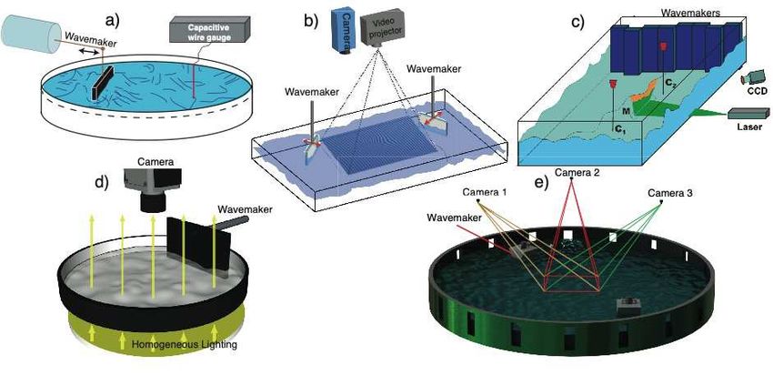
1. INTRODUCTION
    Wave turbulence is generically a statistical state made of a large number of random nonlin-
    early coupled waves. The canonical example is ocean waves. Stormy winds excite large-scale
    surface gravity waves and, due to their nonlinear interaction, the wave energy is redis-
    tributed to smaller scales. This energy transfer leads ultimately to an energy cascade from
    the large (forcing) scale down to small (dissipative) scales.
        Weak turbulence theory was developed in the 1960s to describe the statistical properties
    of wave turbulence in the limits of both weak nonlinearity and an infinite system. It was
    initially motivated to model the ocean wave spectrum (Hasselmann 1962) and has since
    been applied in almost all domains of physics involving waves (see books by Zakharov et al.
    (1992), Nazarenko (2011)). Despite its success at deriving a statistical theory and an-
    alytically predicting the wave spectrum in an out-of-equilibrium stationary state, weak
    turbulence theory does not capture all phenomena observed in nature or in the laboratory.
    For instance, the formation of strongly nonlinear structures (called coherent structures)
    such as sharp-crested waves, result from strong correlations of phases between waves, which
    is at odds with the theoretical hypotheses. For a long time, measurements were mostly
    restricted to single-point measurements that limited the wave field analysis and specifically
    the detection of such coherent structures. The last decade has seen the development of
    measurements simultaneously resolved in space and time that shed new light on the field of
    wave turbulence. These have indeed opened the possibility of probing in detail the spectral
    content of turbulent wave fields simultaneously in wavevector k and frequency ω space,
    as required to discriminate propagating waves from other structures with distinct dynam-
    ics. Following these developments, experiments have explored a broader range of systems
    beyond water waves including vibrating plates (Cobelli et al. 2009b), hydroelastic waves
    (Deike et al. 2013), inertial waves in rotating fluids (Monsalve et al. 2020), and internal
    waves in stratified fluids (Savaro et al. 2020, Davis et al. 2020) (this list being far from ex-
    haustive), not to mention the numerical simulations. It is not an exaggeration to claim that
    the topic of wave turbulence is blooming nowadays.
        Here, we focus our review on experiments concerning gravity-capillary waves at the
    surface of a fluid. Laboratory experiments are restricted to wavelengths typically smaller
    than a meter, even in large-scale wave basins. At these scales the physics is rendered highly
    complex by the interplay of many physical effects. First, waves are supported either by
    gravity or by capillarity, with a transition at wavelengths close to the centimeter scale, at
    which the two contributions are deeply entangled. Second, the finite-system size effects in-
    duce the existence of discrete Fourier modes that affect the energy cascade. Third, viscous
    dissipation, often strongly amplified by surface contamination, also alters the energy flux
    cascading through the scales. Finally, the degree of nonlinearity required for the develop-
    ment of wave turbulence at the surface of water in experiments is not vanishingly weak as
    assumed in theory, and this may lead to the formation of coherent structures in addition
    to waves. Due to new experimental techniques developed since the turn of the twenty-first
    century, the interplay of all these effects can now be explored. In this article, we review the
    experimental works of the last two decades that address all these aspects of wave turbu-
    lence. Complementary details can be found in previous reviews on wave turbulence (Falcon
    2010, Newell & Rumpf 2011, Nazarenko & Lukaschuk 2016, Falcon 2019, Zakharov et al.
    2019, Galtier 2020) or theoretical textbooks (Zakharov et al. 1992, Nazarenko 2011).
        The review is organized as follows. We first describe briefly in Section 2 the general
    features of gravity-capillary surface waves, and in Section 3 we look at the fundamental

2   E. Falcon & N. Mordant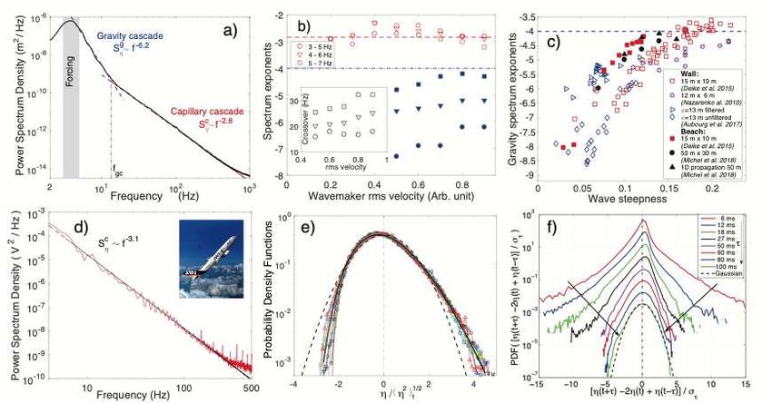
mechanism of wave turbulence, i.e., the nonlinear wave interactions. We then introduce in
Section 4 the phenomenology and the assumptions of weak turbulence theory, and we discuss
in Section 5 the various timescales involved in wave turbulence. We then present in Section
6 the main experimental techniques, including single-point measurements and space-and-
time-resolved measurements. We discuss the main experimental results in Section 7 and 8
by comparing them with weak turbulence predictions and highlighting the abovementioned
effects not taken into account at the current stage of theoretical developments. Finally, we
present in Section 9 a short discussion of large-scale properties in wave turbulence before
ending with lists of Summary Points and Future Issues.
                                                                                                 Crossover: the
                                                                                                 wavelength λgc or
                                                                                                 frequency fgc at
2. GRAVITY-CAPILLARY DISPERSION RELATION                                                         which the gravity
The linear dispersion relation of inviscid deep-water waves is (Lamb 1932)                       term gk is equal to
                                                                                                 the capillary term
                                                                                                 γ 3
                                           r                                                        k in Equation (1)
                                                      γ 3                                         ρ
                                      ω=       gk +     k ,                                 1.   Gravity wave regime:
                                                      ρ
                                                                                                 wavelengths much
with ω = 2πf the angular frequency, k = 2π/λ the wavenumber, g the acceleration of               larger than λgc for
                                                                                                 which the restoring
gravity, ρ the density of the liquid, and γ the surface tension. The crossover betweenp    the   force is gravity
gravity wave regime and the capillary wave regime occurs for a wavelength λgc = 2π γ/(ρg)
                                                                                                 Capillary wave
close to the centimeter for most fluids. Weak turbulence theory is developed for systems         regime: wavelengths
with a power law dispersion relation (i.e., either pure gravity or pure capillary waves),        much smaller than
which is not the case for the dispersion relation above (Equation 1). For intermediate           λgc for which the
scales (i.e., 0.6 . λ . 5 cm or 6 . f . 40 Hz for water waves) easily observed with tabletop     restoring force is
experiments, both capillary and gravity forces are important and should be taken into            capillarity
account. This coexistence leads to several phenomena related to the non-monotonic feature        Parasitic capillaries:
of the phase velocity ω/k of linear waves such as Sommerfeld precursors (Falcon et al. 2003),    generated near steep
                                                                                                 crests of gravity-
parasitic capillarities (Fedorov et al. 1998), or Wilton waves (Henderson & Hammack 1987).       capillary waves as
The minimum of the phase velocity corresponds p      to the transition between the gravity and   the result of a phase
capillary regimes and it occurs at kgc ≡ ρg/γ (the inverse of the capillary length) or,          velocity matching
                                                       √
equivalently, at the frequency fgc ≡ (ρ/γ)1/4 g 3/4 /( 2π). As the ratio ρ/γ is constant for     between a long
usual fluids, working in high-gravity or low-gravity environments provides a way to tune fgc     gravity-capillary
                                                                                                 wave and a shorter
significantly and expand the observation ranges of gravity wave turbulence (Cazaubiel et al.     capillary one
2019b) or of capillary wave turbulence (Falcón et al. 2009).

                                                                                                 Wave steepness ε:
3. NONLINEAR WAVE RESONANT INTERACTIONS                                                          ε ≡ kp ηrms with kp
                                                                                                 the wavenumber at
Resonant interactions between nonlinear waves constitute the fundamental mechanism that          the spectrum peak
transfers energy in weak nonlinear wave turbulence. Generally speaking, N waves interact         (maximum) and
with each other when the following conditions on angular frequencies ωi and on wavevectors       ηrms the standard
                                                                                                 deviation of the
ki are satisfied
                                                                                                 wave elevation

            k1 ± k2 ± ... ± kN = 0 and ω1 ± ω2 ± ... ± ωN = 0, with N ≥ 3.                  2.

Each wave follows the dispersion relation (Equation 1) as well, so that ωi = ω(|ki |). The
magnitude of the nonlinear effects is quantified by the wave steepness ε, and the weak wave
turbulence theory is based on an asymptotic expansion in ε. As a result, it only captures
the dominant nonlinear interactions characterized by a single value of N : N is thereafter

              www.annualreviews.org • Experiments in Surface Gravity-Capillary Wave Turbulence   3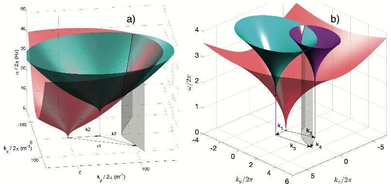
Figure 1
Graphical solutions of Equation (2) for N -wave resonant conditions. (a) An N = 3 solution of Equation (1) exists for
gravity-capillary waves (shown) or for pure capillary waves (ω ∼ k 3/2 ; not shown), but (b) only an N = 4 solution exists
for gravity waves (ω ∼ k 1/2 ). Panels adapted from (a) Aubourg & Mordant (2016) and (b) Aubourg et al. (2017) with
permission from (a,b) American Physical Society.

                         the smallest integer for which Equation 2 has non trivial solutions for a given ω(k) law.
Resonant
                         The different signs ± need to be the same in each instance of Equation 2.
interactions: the two
conditions of                As first suggested by Vedenov (1967) and disseminated by Nazarenko (2011), Equation 2
Equation 2 are           can be solved graphically. Three-wave resonant interactions are only possible if ω(k1 =
satisfied exactly        k2 + k3 ) = ω(k2 ) + ω(k3 ) has a solution, i.e., if the surface ω(kx , ky ) (in red in Figure
with all waves           1a) has a nonempty intersection with the same surface (in blue) in a reference frame whose
following the
                         origin is on ω(k2 ). For pure power laws ω = akb this is only possible for b > 1. In particular,
dispersion relation
                         three-wave resonant interactions occur for capillary waves (b = 3/2), but they are forbidden
Nonresonant
                         for pure gravity waves (b = 1/2) and thus four-wave interactions must be considered (see
interactions: the two
conditions are           Figure 1b). However at scales near the crossover, nonlocal interactions can exist involving
fulfilled but at least   three-wave resonances between a gravity wave and two capillary waves due to the change
one of the involved      of curvature of the dispersion relation (Equation 1) (McGoldrick 1965, Simmons 1969).
Fourier modes is not     Furthermore, unidirectional interactions (i.e., collinear wave vectors ki ) are allowed (which
a free wave (it does
                         are not possible for pure power laws with b 6= 1).
not follow the
dispersion relation).        To extend early experiments on gravity wave resonances (Longuet-Higgins & Smith
                         1966, McGoldrick et al. 1966, Tomita 1989), Bonnefoy et al. (2016) performed experiments
Nonlocal
interactions: the        on four-wave resonant interactions among surface gravity waves crossing in a large basin (see
wavelengths of           Figure 2a-b). This experimentally validated the theory of four-wave resonant interactions
interacting waves        (Phillips 1960, Longuet-Higgins 1962) for a wave steepness smaller than 0.1. Generating
have very different      mother waves of a resonant quartet, they observed the growth of a daughter wave in the ex-
orders of magnitude
                         pected direction (see Figure 2c) and, notably, characterized its resonant properties (growth
contrary to those
involved in local        rate, response curve with the angle, and phase locking between waves). For stronger non-
interactions.            linearities, departures from this weakly nonlinear theory were observed such as additional
                         daughter wave generation by nonresonant interactions (Bonnefoy et al. 2017), which have
                         been well described theoretically by Zakharov & Filonenko (1968) (see Figure 2d).

                     4   E. Falcon & N. Mordant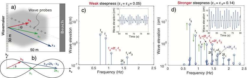
Figure 2
Nonlinear wave interaction. (a) Mother gravity waves are generated at k1 , k2 = k1 and k3 , crossing at an angle θ in a
large-scale basin. Wave probes are located in the expected direction of the daughter wave (k4 ) that should satisfy the
four-wave resonant conditions (2k1 − k3 = k4 and 2ω1 − ω3 = ω4 ), graphically solved as (b) Phillips (1960) so-called figure
of eight. (c) For weak nonlinearity (ε = 0.05), the wave elevation spectrum shows the observation of a daughter wave
(f4 = 2f1 − f3 ) as well as second-order harmonics of the mother waves (2f3 , f1 + f3 , i.e., so-called bound waves). (d) For
stronger nonlinearity (ε > 0.1), there is pumping of a mother wave by daughter ones, and a cascade of quasi-resonances
between mother waves (f1 or f3 ) and primary daughter waves (f4 ), then with secondary daughter waves (f5 ) and (f6 ),
and so on. Insets: Typical wave elevation monitored at the same distance. Panels adapted from (a,b,c) Bonnefoy et al.
(2016) and (d) Bonnefoy et al. (2017) with permission from (a,b,c) Cambridge University Press and (d) EDP Sciences.

     For capillary waves, the inviscid theory of three-wave resonant interactions (McGoldrick
                                                                                                       Quasi-resonant
1965, Simmons 1969) has been tested qualitatively in early experiments (McGoldrick 1970,
                                                                                                       interactions: the two
Henderson & Hammack 1987) and then verified quantitatively experimentally and extended                 conditions of
to more general cases by Haudin et al. (2016) and Abella & Soriano (2019).                             Equation 2 are
     For pure gravity or capillary waves, as for all dispersive waves, resonant interactions           approximately
following Equation 2 involve waves propagating in distinct directions. However, close to               fulfilled, with weak
                                                                                                       nonlinear or
the gravity-capillary crossover, unidirectional resonant interactions involving a gravity wave
                                                                                                       dissipative
and two capillary waves are possible and have been observed experimentally to be the most              corrections to the
active (Aubourg & Mordant 2015, 2016).                                                                 dispersion relation
     Although weak turbulence theory is restricted to strict resonant wave interactions in the
limit of vanishing ε, quasi-resonant coupling among waves is also found to play a significant
role in experiments. As discussed in Section 8, nonlinear widening of the dispersion relation
at a nonzero value of ε enables approximate resonances. Another physical mechanism is
dissipation that increases the resonance bandwidth (as for the damped forced oscillator)
and authorizes three-wave interactions at nonresonant angles (Cazaubiel et al. 2019a).

4. WEAK TURBULENCE THEORY
4.1. Kinetic Equation
Details on the development of weak turbulence theory can be found for instance in
the textbooks by Zakharov et al. (1992) and Nazarenko (2011) and in the review by
Newell & Rumpf (2011). The Hamiltonian equation in Fourier space reads i ∂a    k
                                                                              ∂t
                                                                                     ∂H
                                                                                  = ∂a ∗,
                                                                                       k
with H the Hamiltonian of the system and ak the canonical variables associated with com-
plex wave amplitudes in Fourier space. An asymptotic expansion of the Hamiltonian, using

               www.annualreviews.org • Experiments in Surface Gravity-Capillary Wave Turbulence        5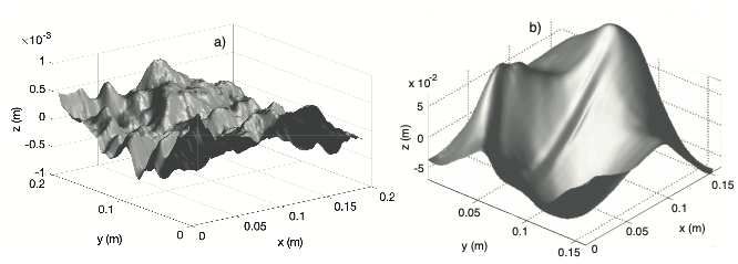
a scale separation hypothesis between the slow time of nonlinear interactions and the fast
                        time of linear wave oscillations, leads to
                                                                Z
                                         ∂ak     ∂H
                                       i       =     = ωak + ε Vk,k1 ,k2 ak1 ak2 δ(k1 + k2 − k)dk1 k2
                                          ∂t     ∂ak
                                                   ∗
                                             Z                                                                  3.
                                       +ε2 Wk,k1 ,k2 ,k3 ak1 ak2 ak3 δ(k1 + k2 + k3 − k)dk1 k2 k3 + ...,

                        with Vk,k1 ,k2 the three-wave interaction coefficient and Wk,k1 ,k2 ,k3 the four-wave interaction
                        coefficient (Hasselmann 1962, Zakharov et al. 1992, Nazarenko 2011). For ε ≪ 1, one can
                        consider only the smallest nonzero coefficient in this development. As discussed above,
                        N = 3 for capillary waves and N = 4 for gravity waves. To reach statistical properties,
                        weak turbulence theory computes the second-order moment of the canonical variable hak ak’ i
                        using the random phase hypothesis (wave phase and amplitude are assumed quasi-Gaussian)
                        (Nazarenko 2011) or the hierarchy of the cumulants of the canonical variables (Newell et al.
                        2001), where h·i denotes a statistical average. Assuming spatial homogeneity and based on
                        the linear and nonlinear timescale separation hypothesis, an asymptotic closure arises in the
                        limit of infinite system size and of vanishing nonlinearity. The resulting kinetic equation
                        describing the long-time evolution of the wave action spectrum nk = hak a∗k i reads, for
                        three-wave interactions (capillary case)
                                        Z
                          ∂nk                                                          1      1       1
                               = 4πε2 |Vk,k1 ,k2 |2 nk nk1 nk2 δ(k − k1 − k2 )            −       −        δ(ω − ω1 − ω2 )+
Kinetic equation:          ∂t                                                         nk    nk1      nk2
equation for the slow
                                 1       1     1                               1     1      1
temporal evolution                  −       +          δ(ω1 − ω − ω2 ) +         +       −        δ(ω2 − ω1 − ω) dk1 dk2 ,
of the wave action              nk     nk1    nk2                             nk    nk1    nk2
spectrum nk                                                                                                                4.
                          and, for four-wave interactions (gravity case),
                                        Z
                          ∂nk         4                    2                                       1      1     1      1
                               = 4πε       |Wk,k1 ,k2 ,k3 | nk nk1 nk2 nk3 δ(k + k1 − k2 − k3 )       +      −      −
                           ∂t                                                                     nk     nk1   nk2    nk3
                                                                                    δ(ω + ω1 − ω2 − ω3 )dk1 dk2 dk3 ,
                                                                                                                    5.
                        Note that the collision integral contributes to the spectrum evolution only when the resonant
                        interaction conditions are satisfied due to Dirac’s δ functions. For the complete gravity-
                        capillary system, most likely both terms should be taken into account, although it has never
                        been investigated.

                        4.2. Constant Flux Solutions
                        By definition of canonical variables, the spectral energy density (or wave energy spectrum)
                        Ek is related to the wave action spectrum nk by Ek = ω(k)nk , the total wave energy
                              R
                        E = Ek dk being conserved. The energy flux P is defined by the following balance:
                        ∂Ek
                         ∂t
                            + ∂P
                               ∂k
                                   = 0. Stationary solutions of the kinetic equation cancel the collision integral and
                        thus correspond to a constant energy flux P across scales (in practice, between the energy
                        source and sink). For power law dispersion relations, ω = akb , Zakharov’s transformation
                        (Zakharov et al. 1992, Nazarenko 2011) provides the stationary isotropic solutions as power
                        laws in k
                                                        nk = 2πC0 P 1/(N−1) a−α k−β ,                                6.
                        where N is the leading-order interaction in the system, C0 , α, and β are constants
                        that can be computed and that depend on the wave system considered. By analogy to

                   6    E. Falcon & N. Mordant
the Kolmogorov spectrum in 3D hydrodynamic turbulence, these solutions are called the
Kolmogorov-Zakharov (KZ) spectra.
Since the exact analytical computation of the above solutions is rather long and techni-
cal, one way to find the KZ spectrum scalings is to use dimensional analysis (Zakharov et al.
Kolmogorov-
1992, Connaughton et al. 2003, Nazarenko 2011). Let us consider waves propagating in two Zakharov (KZ)
dimensions according to ω = akb , where the dimension of a is Lb T −1 . The dimension of
4 −2 spectra:
the energy density Ek , normalized by unit of surface and density, is L T . The energy constant flux,
flux P , similarly normalized, has the dimension L3 T −3 . For a system dominated by N out-of-equilibrium,
wave interactions, the energy flux is proportional to the power N − 1 of the spectral energy stationary solutions
1 of the kinetic
density (and thus Ek ∼ P N −1 ) (Kraichnan 1965, Connaughton et al. 2003). Dimensional equation
analysis thus yields
1
Ek ∼ P N −1 aξ kζ , with ξ = 2 − 3/(N − 1) and ζ = 2b − 4 + (3 − 3b)/(N − 1). 7.
One has also β = b − ζ and α = 1 − ξ. Most experiments rather consider the power spectral
RR L 2 RT 2
density Sk = 2πkh 0 η(x, y)ei(kx x+ky y) dxdy i/L2 or Sω = h 0 η(t)ei(ωt) dt i/T of the
measured wave elevation η(x, y) or η(t), L being the window size and T the recording time.
Sk is related to the energy spectrum by Ekg = 12 gSkg for gravity waves, and Ekc = 2ρ γ 2 c
k Sk
for capillary waves. These densities can be changed to frequency space using Ek dk = Eω dω
and Sk dk = Sω dω and the linear dispersion relation. For deep-water gravity waves (N = 4,
√
b = 1/2, a = g), Equation 7 thus yields the spectrum predictions of the direct energy
cascade
Ekg ∼ P 1/3 g 1/2 k−5/2 , Skg ∼ P 1/3 g −1/2 k−5/2 , Sωg ∼ P 1/3 gω −4 . 8.
The exact solution was derived by Zakharov & Filonenko (1967a). For capillary waves
[N = 3, b = 3/2, a = (γ/ρ)1/2 ], the spectrum predictions are
1/4 −3/4 1/6
γ γ γ
Ekc ∼ P 1/2 k−7/4 , Skc ∼ P 1/2 k−15/4 , Sωc ∼ P 1/2 ω −17/6 . 9.
ρ ρ ρ
The exact solution was derived by Zakharov & Filonenko (1967b).
The nondimensional KZ constant C0 was estimated experimentally for gravity waves
by Deike et al. (2015) and found to be of the same order of magnitude as the theoretical
value (C0g = 2.75) estimated by Zakharov (2010). For capillary waves, the KZ constant
was first analytically evaluated as 9.85 by Pushkarev & Zakharov (2000) and corrected by
Pan & Yue (2017) to C0c = 6.97. Using a low dissipation level, direct numerical simulation
by Deike et al. (2014b) led to C0c = 5 ± 1, whereas Pan & Yue (2014) found a value that
depends on the system’s finite size. Experimental estimation of the KZ capillary constant
(see Section 7.2) led to C0c ≈ 0.5 (Deike et al. 2014a).
For the full gravity-capillary system, since the dispersion relation is not a pure power
law, so far no analytical solution for the KZ spectrum exists, and dimensional analysis is
not conclusive. One may expect to recover the pure gravity or capillary cases at scales
far from the crossover but the connection between the two solutions in the intermediate
region remains unclear. Because the scalings in P of the two pure cases are different, one
may expect the transition between both regimes to occur at distinct scales when changing
the energy flux. When equating the two KZ spectra of Equations 8 and 9, one obtains
the transition between the two spectra Sk at k = kgc (C0c /C0g )4/5 (P/Pb )2/15 , where Pb =
www.annualreviews.org • Experiments in Surface Gravity-Capillary Wave Turbulence 7(γg/ρ)3/4 is the energy flux breaking weak turbulence (see Section 5.1). The transition
Conservation of the
number of
should thus slightly increase with P and be equal to kgc only for P = Pb (C0g /C0c )6 ≃ Pb /265.
interacting waves: When N is even and a conservation of the number of interacting waves occurs (as for
R
for N = 3, the gravity waves), the total wave action N = nk dk is conserved as well, and the wave action
number of flux Q is defined as ∂n∂t
k
+ ∂Q
∂k
= 0. An inverse cascade (from small scales to large ones)
interacting waves is is then predicted characterized by a constant wave action flux through the scales once
never conserved
(2 ↔ 1 process); for
a stationary state is reached. Since [Q] = [P ]/[ω], the dimension of Q is [L3 T −2 ], and
N = 4, it is either dimensional analysis leads to the inverse cascade spectrum
conserved (2 ↔ 2) or 1
not (3 ↔ 1) Eki ∼ Q N −1 aξ kζ , with ξ = 2 − 2/(N − 1) and ζ = 2b − 4 + (3 − 2b)/(N − 1). 10.
√
For deep-water gravity waves (N = 4, b = 1/2, a = g), the inverse cascade spectra are
Eki ∼ Q1/3 g 2/3 k−7/3 , Ski ∼ Q1/3 g −1/3 k−7/3 , Sωi ∼ Q1/3 gω −11/3 . 11.
The exact solution was derived by Zakharov & Zaslavskii (1982).
4.3. Zero-Flux or Independent-Flux Solutions
Other solutions of the wave action spectra exist beyond those of Section 4.2. For example, for
capillary waves, no inverse cascade is predicted (N = 3 is odd), and the dynamics at scales
larger than the forcing scale is thus expected to follow the statistical (or “thermodynamic”)
equilibrium state, that is, the kinetic energy equipartition among the Fourier modes with no
wave action flux towards large scales (Balkovsky et al. 1995). The spectrum of large-scale
capillary wave turbulence is thus predicted as Skth = kB T /(2πσk) or Sωth = 2kB T /(3σω)
(Michel et al. 2017) with kB the Boltzmann constant and T a constant effective temperature
related to the total energy within this out-of-equilibrium stationary state. This is the analog
of the Rayleigh-Jeans spectrum of the blackbody radiation.
Beyond weak turbulence, a flux-independent solution for gravity waves was proposed di-
mensionally by Phillips (1958) as SωP h ∼ P 0 g 2 ω −5 . It is interpreted as a saturated spectrum,
a situation that in practice corresponds to nonlocal interactions where localized coherent
structures (whitecaps, wave breaking) associated with steep gravity waves dissipate all the
injected energy (Newell & Rumpf 2011). At intermediate stages (between weak turbulence
and saturation) Kuznetsov (2004) proposed that the spectrum would be proportional to the
density n of singularities with an exponent in k that depends on the geometry of the struc-
tures. If these dissipative structures occur along lines rather than locally (sharp-crested
waves) then SωK ∼ nω −4 is expected (Kuznetsov 2004, Nazarenko et al. 2010). Numerical
simulations have shown some evidence of Phillips’ spectrum in the inverse cascade regime
(Korotkevitch 2008, Korotkevich 2012).
5. TIMESCALES OF WAVE TURBULENCE
Weak turbulence theory assumes a timescale separation τlin (k) ≪ τnl (k) ≪ [τdiss (k) and
τdisc (k)]. In the whole inertial range, the timescale of nonlinear interactions between waves,
τnl , is assumed to be large compared with the linear time, τlin = 1/ω, so that the nonlinear
evolution is slow compared with the fast linear oscillations of the waves. In addition, τnl
must be short compared to the typical dissipation time τdiss and the discreteness time τdisc .
Let us discuss all these time scales.
8 E. Falcon & N. Mordant5.1. Nonlinear Timescale
From scaling arguments on the kinetic equation, the nonlinear interaction time reads
(Newell & Rumpf 2011)
g
τnl ∼ P −2/3 g 1/2 k−3/2 (gravity), and τnl
c
∼ P −1/2 (γ/ρ)1/4 k−3/4 (capillary). 12.
g
For gravity waves, one must have τlin /τnl ∼ P 2/3 k1 /g ≪ 1 (Newell & Rumpf 2011). As
this ratio increases with k, breakdown of the weak nonlinearity hypothesis is expected to
occur at small scales for k > kbg ∼ g/P 2/3 . By contrast, for capillary waves, breakdown
c
occurs at large scales since the ratio τlin /τnl ∼ P 1/2 (kγ/ρ)−3/4 ≪ 1 decreases with k and
thus exceeds one for k < kbc ∼ P 2/3 ρ/γ. At small enough P one has kbg > kbc , and thus
a weak regime of gravity-capillary turbulence may develop at all scales. Equating these
two breaking scales, kb = kbg = kbc , leads to a critical energy flux, Pb = (γg/ρ)3/4 , that
breaks weak gravity-capillary wave turbulence (Newell & Zakharov 1992). For P > Pb ,
one has kbg < kbc and a window in k-space exists (typically k ∈ [kbg , kbc ], near the gravity-
capillary transition) where the dynamics is expected to be dominated by strongly nonlinear
structures (white caps, sharp-crested waves) (Newell & Zakharov 1992, Connaughton et al.
2003) or by nonlocal interactions, such as parasitic capillary wave generation (Fedorov et al.
1998), as evidenced experimentally by the occurence of stochastic energy bursts trans-
ferring wave energy non-locally from gravity waves to all capillary spatial scales quasi-
instantaneously (Berhanu & Falcon 2013, Berhanu et al. 2018). However, no such transition
from a weak turbulence spectrum to a strong turbulence spectrum (Phillips’ spectrum) at
high wave numbers has been reported experimentally so far. This independent-flux solution
(i.e., Phillips’ spectrum of sharp, crested waves) has a k-independent ratio, τlin /τnl ∼ k0
(Newell & Rumpf 2011). For usual fluids, Pb is roughly constant, about 4200 cm3 /s3 . Ex-
perimentally, the cascading energy flux P can be indirectly measured (see Section 7.2)
and is found to be more than one order of magnitude smaller than the critical flux Pb
(Deike et al. 2015, Cazaubiel et al. 2019b). The value of τnl can be measured with a local
probe by decaying wave turbulence experiments either in the gravity regime (Bedard et al.
2013, Deike et al. 2015) or in the gravity-capillary regime (Cazaubiel et al. 2019b), and by
the broadening of the dispersion relation in stationary experiments using space-time mea-
surements (Herbert et al. 2010, Berhanu et al. 2018). In the latter case, the width of the
energy concentration around the dispersion relation can be quantified either in frequency
∂k
space by δω ∝ 1/τnl or in wavenumber space by δk ∝ ∂ω δω.
Similarly, for the inverse cascade of gravity waves, the nonlinear timescale reads
i
τnl ∼ g 1/6 Q−2/3 k−11/6 , and thus we have the ratio τlin /τnl i
∼ Q2/3 g −2/3 k4/3 ≪ 1
(Newell & Rumpf 2011). As this ratio increases with k or with the wave action flux p Q,
breakdown of weak turbulence is expected to occur at small scales when k > kb = g/Q
or for Q > Qb = g/k2 . Here also, wave action flux in experiments is much smaller than this
critical value (Falcon et al. 2020).
5.2. Dissipation Time
The scale separation τnl (k) ≪ τdiss (k) is taken for granted in the theory but it is not so
straightforward in real life. Energy dissipation in water waves occurs mainly through three
distinct mechanisms: viscous linear damping (very small for large-scale waves λ & 0.5
m), energy extraction by generation of parasitic capillaries near steep crests of longer
waves (Longuet-Higgins 1963, Fedorov et al. 1998), and wavebreaking (i.e., a multival-
www.annualreviews.org • Experiments in Surface Gravity-Capillary Wave Turbulence 9ued interface) at very large steepnesses. When assuming a stress-free water/air interface,
the typical linear viscous dissipation timescale is due the water bulk viscosity and thus
we have τdiss = 1/(2νk2 ) (Lamb 1932, Miles 1967, Deike et al. 2012). For a contami-
nated interface, the air/water surface boundary layer due to an inextensible film gives
s
√ √
τdiss = 2 2/(k νω) (van Dorn 1966, Henderson & Miles 1990) [which is negligible for
f . 2 Hz (Campagne et al. 2018)]. The boundary layer on the lateral walls (for exper-
L
√ √
iments) yields τdiss = 2 2Lx Ly /[3 νω(Lx + Ly )] (Miles 1967, Cazaubiel et al. 2019b),
whereas the bottom boundary layer dissipation is negligible for deep-water waves. The
term τdiss is usually measured with a local probe by decaying wave turbulence experiments
either in the gravity regime (Bedard et al. 2013, Deike et al. 2015), in the gravity-capillary
regime (Cazaubiel et al. 2019b), or in the capillary regime (Deike et al. 2012).
5.3. Discreteness Time
Finite-size effects often play a role in wave turbulence experiments, as the presence of con-
fining lateral walls cannot be avoided. A closed basin exhibits eigenmodes that depend on
its size and geometry. Indeed, the boundary conditions lead to a discretization of possible
wave q vectors. For example, for a rectangular basin of size Lx and Ly , the eigenmodes are
kd = (mπ/Lx )2 + (nπ/Ly )2 with m, n ∈ N (Lamb 1932). The discreteness time τdisc can
be computed as the number of eigenmodes found in a frequency band divided by this band-
width (Falcon et al. 2020). When the nonlinear spectral widening δk is greater than the half
separation ∆k/2 between adjacent eigenmodes, they are no longer separated and this pre-
vents any effect of discreteness. It occurs when τnl (k) < 2τdisc (k), with τdisc = 1/∆ω and
∆ω = (∂ω/∂k)∆k. In this case, one expects to recover a kinetic regime with effectively con-
tinuously varying wavenumbers as in the limit of infinite system size considered in the theory.
In the opposite case, τnl (k) > 2τdisc (k), discrete wave turbulence is expected. The interme-
diate regime, τnl ∼ 2τdisc , is called “frozen” or “mesoscopic” wave turbulence (Nazarenko
2011). For instance, pin a system of size L, one has ∆k = π/L, andp the discreteness time
g c
reads τdisc = (2L/π) k/g for gravity waves and τdisc = [2L/(3π)] ρ/(γk) for capillary
waves (Ricard & Falcon 2021b). The frozen scale occurs for τnl (kf r ) = 2τdisc (kf r ), that is,
using both parts of Equation 12, kfg r = πg/(4L)P −1/3 and kfc r = [3π/(2L)]4 (γ/ρ)3 P −2 for
p
each regime (Ricard & Falcon 2021b). The finite-system size effects are thus more significant
when L or P decreases. Taking these effects into account in theories is an important chal-
lenge (Zakharov et al. 2005, Nazarenko 2006, Kartashova et al. 2008, L’vov & Nazarenko
2010, Pan & Yue 2017, Hrabski & Pan 2020).
5.4. Timescale Separation
The physical properties of water provide constraints on the scale separation. For large-
scale gravity waves (λ > 1 m), one has τlin /τdiss < 10−5 since the dissipation due to bulk
viscosity is almost negligible (Campagne et al. 2018), and one thus expects a proper scale
separation in field observations at these scales. In laboratory experiments, the system size
most often restricts the studied scales to wavelengths below 1 m, even in large-scale tanks.
Near the crossover and for smaller wavelengths, the ratio is τlin /τdiss & 10−2 for water, and
further increases in the case of surface contamination (Campagne et al. 2018). This means
that the forcing (and so the wave steepness) must be high enough to reach an adequate scale
separation (τlin ≪ τnl ≪ τdiss ) at these wavelengths, at the risk of not being so weakly
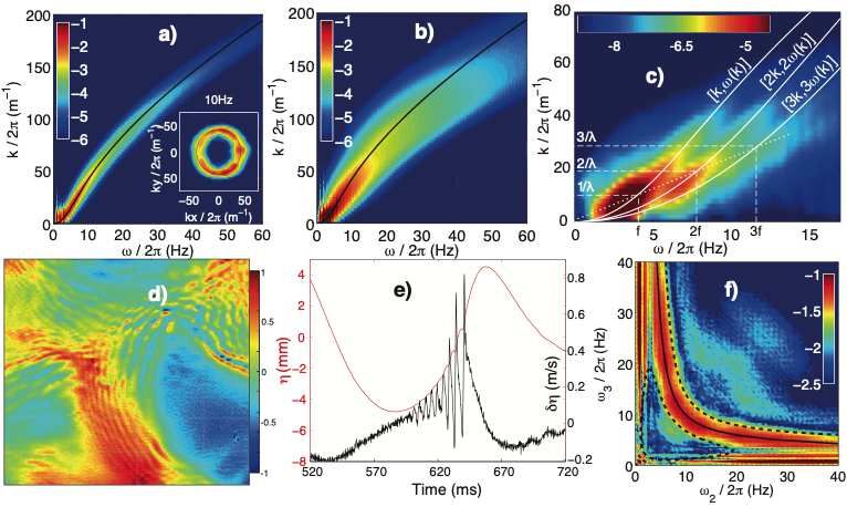
10 E. Falcon & N. MordantFigure 3
Typical surface wave elevation measurements: (a) capacitive wire gauge, (b) 3D wave field reconstruction by Fourier
Transform Profilometry (FTP), (c) 2D spatial profile, (d) 3D Diffusing Light Profilometry (DLP), and (e) 3D stereo-PIV.
Panels adapted from (a) Cazaubiel et al. (2019b), (b) courtesy from P. Cobelli, (c) Nazarenko et al. (2010), (d) courtesy
from J.-B. Gorce, (e) Aubourg et al. (2017) with permission from (a,d,e) American Physical Society.
nonlinear (typically ε ≃ 0.05 − 0.1). To decrease capillary viscous dissipation, researchers
have performed experiments with mercury (Falcon et al. 2007b,a, 2008, Ricard & Falcon
2021a), or with liquid hydrogen (Brazhnikov et al. 2002, Kolmakov et al. 2009). A direct
estimation of the nonlinear timescale is not straightforward and was accomplished only in
a few cases (see Section 5.1). The timescale separation was found to be well validated
experimentally for gravity wave turbulence (Deike et al. 2015, Falcon et al. 2020) and for
gravity-capillary wave turbulence (Cazaubiel et al. 2019b), as well as numerically for pure
capillary wave turbulence (Deike et al. 2014b) [see also Deike et al. (2013) and Miquel et al.
(2014) for such tests in other experimental wave turbulence systems]. However, when the
finite-size effects are significant, the nonlinear and dissipative timescales are found to be
independent of the scale, contrary to weak turbulence predictions (Cazaubiel et al. 2019b).
6. EXPERIMENTAL METHODS
Water waves are commonly generated by a localized forcing using a wave maker made of one
or multiple independently controlled paddles (see Figure 3). Injected power into the fluid
can be measured (Falcon et al. 2008), as can the energy flux P , indirectly (see Section 7.2).
6.1. Single-Point Measurements
In field observations, surface wave elevations are usually measured by buoys, lidar or mi-
crowave radars. In laboratory experiments, resistive or capacitive wire gauges are widely
www.annualreviews.org • Experiments in Surface Gravity-Capillary Wave Turbulence 11used (see Figure 3a). Capacitive probes are made of a thin insulated wire in water, con-
sidered as an annular capacitor with a capacity proportional to the immersed length of
the wire. Although intrusive, they are easy to implement and have a wide measurement
range (from 10 µm to tens of cm with a frequency cutoff up to a few hundred Hz and no
limitation in wave steepness) (Falcon et al. 2007b,a, Deike et al. 2012). They are more ad-
equate for small-scale resolution than resistive probes, which are restricted to gravity wave
studies. The resistive probe accuracy for the height detection is . 100 µm with a rather
low frequency cutoff . 20 Hz (Cazaubiel et al. 2019b).
To avoid possible disruption of the wave field by gauges, several authors have used
nonintrusive optical methods based on tracking by a position-sensitive detector of the par-
tial adsorption (Henry et al. 2000), reflection (Lommer & Levinsen 2002, Brazhnikov et al.
2002, Kolmakov et al. 2009), or refraction (Snouck et al. 2009) of a laser beam at one point
of the fluid surface to study capillary wave turbulence with a parametric forcing. Other
authors have used single-point laser Doppler vibrometers to study capillary wave turbu-
lence (Holt & Trinh 1996), depth-induced properties in gravity-capillary wave turbulence
(Falcon & Laroche 2011), wave turbulence in a two-layer fluid (Issenmann et al. 2016), and
gravity-capillary wave resonant interactions (Haudin et al. 2016, Cazaubiel et al. 2019a).
Laser vibrometry consists in a reference laser beam that interferes with light backscattered
by the moving free surface. It infers the normal wave velocity by the Doppler effect and
the wave elevation by interferometry, with high displacement measurement accuracy (up to
∼ 0.3 µm or 0.1 µm/s), thin spatial extension of the probe region of the order of 10µm, that
is a few times the laser beam diameter, and a high temporal dynamics (timescales down to
∼ µs). It requires the addition of light scattering particles in water and is limited to low
wave steepness (< 0.1).
Beyond the above Eulerian specifications of the wave field, recent articles report the
use of particle tracking velocimetry of Lagrangian buoyant particles or floaters to study
gravity-capillary wave turbulence (Del Grosso et al. 2019, Cabrera & Cobelli 2021).
6.2. Space-Time Measurements
Simultaneous measurements in the time and space domains enable one to discriminate
weakly nonlinear waves that verify the dispersion relation from other more complex dy-
namics.
Space-and-time-resolved imaging of the free surface along a line can be achieved by
using a laser sheet impinging the water surface (Lukaschuk et al. 2009) (see Figure 3c) or
scanning a laser beam refracted by the free surface (Snouck et al. 2009). In linear flumes
with transparent side walls, laterally positioned cameras can image the 2D spatial profile
along the flume (Redor et al. 2020, Ricard & Falcon 2021a).
Nowadays, full 3D spatial wavefield reconstructions are achieved using high-speed cam-
eras. The Fourier Transform Profilometry (FTP), introduced by Takeda & Mutoh (1983)
and further developed by Cobelli et al. (2009a), was used by Herbert et al. (2010) to obtain
the nonlinear dispersion relation and spatial statistics of gravity-capillary wave turbulence.
It is now the most widespread 3D reconstruction technique for small-scale experiments
(Cobelli et al. 2009b, 2011, Deike et al. 2013, Aubourg & Mordant 2015). The principle is
to project a grayscale pattern made of parallel lines at the water surface. A fast camera
records the pattern deformed by the waves; the water height can be recovered by a de-
modulation algorithm (see Figure 3b). The spatial horizontal resolution is of the order
12 E. Falcon & N. Mordantof the distance between the projected lines (few mm, typically) and the resolution of the
measurement of the water elevation is about 100 µm. A white dye must be added to ren-
der the water diffusive to light. A paint dye was first used (Herbert et al. 2010), followed
by titanium dioxide (TiO2 ) particles, which led to much lower modifications of the fluid
properties (surface contamination, viscosity) (Przadka et al. 2012).
Diffusing light photography or profilometry (DLP) is a technique more adapted to cap-
illary wave turbulence since its horizontal and vertical resolution are higher (∼ 10 µm) than
those of FTP. Wright et al. (1996, 1997) introduced DLP to study capillary wave turbu-
lence, but the spatial wave height reconstruction was achieved using photographs with no
temporal resolution (only collections of snapshots). By associating this technique with a
fast camera, Berhanu & Falcon (2013), Haudin et al. (2016), and Cazaubiel et al. (2019a)
obtained the full space-and-time-resolved measurements of gravity-capillary wave turbu-
lence (see Figure 3d). This optical method is based on the light absorption of a diffusing
fluid (water and microspheres). The surface topography is reconstructed from the variations
of the light intensity transmitted through the liquid illuminated from below and captured
by a fast camera from above. Contrary to usual optical methods based on the wave slope
measurement (reflection or refraction), DLP works well for steeply sloping waves and is thus
well adapted to study strong capillary wave turbulence (Berhanu et al. 2018). A similar
absorption technique was implemented at an interface between two index-matched liquids
(a transparent upper liquid and a dyed lower liquid) to reconstruct Faraday surface wave
patterns (Kityk et al. 2004).
Synthetic Schlieren was first developed to image internal waves (Peters 1985,
Dalziel et al. 2000), and has since been applied to image water waves (Kurata et al. 1990,
Moisy et al. 2009) and, more recently, to test surface three-wave resonant interactions
(Abella & Soriano 2019). This method is based on the analysis of the image of a ran-
dom dot pattern (placed below the wave tank) refracted trough the water surface. The
reconstruction of the wave field is obtained using a digital cross-correlation PIV (particle
image velocimetry)-type algorithm. Despite its extreme sensitivity (∼ 1 − 10 µm), this
method based on light refraction provides the gradient of wave height and is thus limited
to small wave steepness (to prevent the formation of caustics) and small wave amplitudes.
Time-and-space-resolved wave field measurements from video using multiple camera
views are currently booming, notably for gravity waves, as in stereoscopy (Benetazzo 2006,
Leckler et al. 2015, Zavadsky et al. 2017) or stereo-PIV (Prasad 2000, Turney et al. 2009,
Aubourg et al. 2017) (the latter requiring tracers, with a vertical resolution ∼ mm, and a
horizontal resolution of a few cm; see Figure 3e).
7. SINGLE-POINT WAVE SPECTRUM
The wave elevation, η(t), measured at a single point of the fluid surface, is generally found
to randomly fluctuate over time. The corresponding spectrum, Sω , leads to power law
scalings coexisting in the gravity and capillary regimes, for high enough nonlinearity (see
Figure 4a). Each regime leads to different conclusions when compared to the predictions
of Equations 8 and 9.
www.annualreviews.org • Experiments in Surface Gravity-Capillary Wave Turbulence 13Figure 4
(a) Experimental gravity-capillary wave spectrum Sω and best fits in the gravity and capillary regimes. fgc is the
crossover frequency. (b) Capillary and gravity exponents of frequency power law spectra as a function of the random
forcing strength and for different forcing bandwidths. Dashed lines correspond to weak wave turbulence predictions. (c)
Wave steepness-dependent gravity exponents in different basin sizes and boundary conditions: open symbols (wall) and
full symbols (beach). (d) Capillary-wave turbulence spectrum, Sω , in low-gravity environment. Wave statistics: (e)
non-Gaussian distribution of dimensionless wave elevation, and (f ) distribution of the dimensionless second-order
differences of wave elevation, η(t + τ ) − 2η(t) + η(t − τ ) over a time lag τ , as a signature of intermittency. Panels adapted
from (a) Cazaubiel et al. (2019b) (b) Falcon et al. (2007b), (d) Falcón et al. (2009), (e) Falcon & Laroche (2011), (f )
Falcon et al. (2007a) with permission of (a,b,f ) American Physical society, (d,e) IOP Science. Panel (c) is an original
creation. Inset of panel (d) courtesy of Novespace.
7.1. Gravity Regime
In the gravity regime, the main experimental observation is that the exponent of the
power law wave spectrum differs significantly from the prediction of Equation 8, Sωg ∼
ω −4 . The exponent was found to depend strongly on the wave steepness in experi-
ments in laboratory basins with sizes ranging from 0.5 to 50 m (Falcon et al. 2007b,
Denissenko et al. 2007, Lukaschuk et al. 2009, Nazarenko et al. 2010, Cobelli et al. 2011,
Deike et al. 2015, Aubourg et al. 2017) (see Figure 4b,c), as well as in field observa-
tions (see, e.g., Huang et al. (1981)). The exponent depends also on the shape of the
basin (Issenmann & Falcon 2013). The gravity spectrum was indeed found to be indepen-
dent of the forcing for a cylindrical container but not for a rectangular one. The role of the
boundary conditions (absorbing, i.e., with a beach, or reflecting, i.e., with a wall) has also
been addressed (Deike et al. 2015). Although the observed stochastic wave field pattern
depends strongly on these boundary conditions, their spectral properties have been found
to be similar (see Figure 4c). This self-similar gravity wave spectrum (depending on the
wave steepness) has been shown to be due to the presence of bound waves (Michel et al.
2018, Campagne et al. 2018) (see also Section 8) instead of free waves. Note that for very
14 E. Falcon & N. Mordantsmall wave steepness (≃ 0.02), the gravity spectrum has been found to be much steeper
Free waves: Fourier
than the weak turbulence prediction, suggesting a strong impact of dissipation, although
modes that follow
care was taken to avoid surface contamination (Aubourg & Mordant 2016). the dispersion
In decaying wave turbulence experiments, the mean energy flux is estimated from relation
the gravity wave energy decay rate. It is observed to be much smaller than the flux Pb Bound waves: in a
breaking weak turbulence theory (see Section 5.1) (Bedard et al. 2013, Deike et al. 2015, stochastic wave field,
Cazaubiel et al. 2019b). Nevertheless a deeper analysis of the space-time spectrum (see bound waves are
Section 8) shows the presence of various structures associated with a finite level of nonlin- generated by
nonresonant wave
earity.
interactions and do
The probability density functions (PDF) of wave elevation are found to be well described not follow the linear
by the first nonlinear correction to a Gaussian distribution (i.e., a Tayfun distribution), as dispersion relation
a confirmation of weak nonlinearity of the wave field but also of the presence of effects of a
small but finite level of nonlinearity [see, e.g., Falcon et al. (2007b) and Figure 4e]. More-
over, intermittency in gravity-capillary wave turbulence has also been reported (Falcon et al.
2007a, Lukaschuk et al. 2009) (see Figure 4f ). High-order differences of wave elevation
need to be used when testing intermittency for signals with steep spectra as in the case of
gravity-capillary waves (Falcon et al. 2010a). This small-scale intermittency is enhanced by
coherent structures (wavebreakings, capillary bursts on steep gravity waves) (Falcon et al.
2010b) and is reduced by the wave directionality level (Fadaeiazar et al. 2018). It also de- Intermittency: when
pends strongly on the forcing (Falcon et al. 2010b, Deike et al. 2015) but not on the basin the probability
density function of
boundary conditions (Deike et al. 2015). Its origin is still an open problem and it may be the wave elevation
related to the fractal dimension of possible singularities (e.g., peaks or wave-crest ridges) increments is
involved in the wave field (Connaughton et al. 2003, Nazarenko et al. 2010). Statistics of Gaussian at large
Fourier modes (in space or in time) also reveals heavy-tail distributions attributed to the scales and departs
presence of large-scale coherent structures (Nazarenko et al. 2010). Finally, numerical sim- strongly from being
Gaussian at small
ulations of weak gravity wave turbulence have confirmed the KZ spectrum of Equation 8 scales
(Dyachenko et al. 2003, 2004).
7.2. Capillary Regime
Capillary wave turbulence was first studied using parametric forcing and optical mea-
surement methods (Holt & Trinh 1996, Wright et al. 1996, 1997, Henry et al. 2000,
Lommer & Levinsen 2002, Brazhnikov et al. 2002, Kolmakov et al. 2009, Snouck et al.
2009, Xia et al. 2010). This peculiar forcing led to a discrete spectrum of peaks with
amplitudes decreasing as a frequency power law, since this forcing does not generate trav-
elling waves and thus cannot be really related to kinetic wave turbulence. The use of
randomly driven wave makers then led to the observation of a continuous power law wave
spectrum with an exponent verifying accurately Equation 9 (Sωc ∼ ω −17/6 ) at moderate
forcing, typically 0.05 . ε . 0.15 (Falcon et al. 2007b, Herbert et al. 2010, Cobelli et al.
2011, Deike et al. 2012, Issenmann & Falcon 2013, Deike et al. 2014a).
For low enough viscosity, the mean energy flux scaling as Sωc ∼ P 1/2 has also been
verified experimentally from the estimation of the dissipated energy spectrum (Deike et al.
2014a). This estimation of the mean energy flux scaling is more reliable than the one esti-
mated from the mean injected power, which includes an unknown amount going in the bulk
of the fluid (Falcon et al. 2007b, Xia et al. 2010, Issenmann & Falcon 2013). Note also that
strong temporal fluctuations of the injected power have been reported (Falcon et al. 2008).
With the P - and ω- scaling agreements, the KZ capillary constant can thus be estimated
www.annualreviews.org • Experiments in Surface Gravity-Capillary Wave Turbulence 15experimentally and is found to be one order of magnitude smaller than the theoretical one
(Deike et al. 2014a) (see Section 4.2). This discrepancy may be ascribed to dissipation
occurring at all scales of the cascade, leading to a nonconstant energy flux (Deike et al.
2014a).
The broadband dissipation is also evidenced in nonstationary wave turbulence experi-
ments. After switching off the wave maker, the energy decay was shown to be mainly driven
by the longest container eigenmodes, each Fourier mode decaying with the same damping
rate (Deike et al. 2012, Cazaubiel et al. 2019b). These long waves provide an energy source
during the decay that sustains nonlinear interactions to keep capillary waves in a turbulent
state with the expected spectrum prediction because nonlinear interactions occur faster at
each scale of the cascade than dissipative processes (see e.g. Cazaubiel et al. (2019b)).
When dissipation increases (higher viscosity fluids), the wave spectrum becomes steeper
and the capillary exponent departs from its theoretical value and depends on the forcing
strength, which is reminiscent of results obtained in the gravity regime (Deike et al. 2012).
For wave turbulence in vibrating plates, the effect of dissipation has also been unambigu-
ously shown to steepen the spectra (Humbert et al. 2013, Miquel et al. 2014).
Pure capillary wave turbulence has been reached experimentally either in low-gravity
environment [in parabolic flight experiments (Falcón et al. 2009) or onboard the Interna-
tional Space Station (Berhanu et al. 2019)], or at the interface of two immiscible fluids of
close densities, either in presence of an additional interface with air (Issenmann et al. 2016)
or without such interface (Düring & Falcón 2009). It leads to an excellent agreement with
the ω −17/6 spectrum on more than two decades within the inertial range for weak enough
forcing (Falcón et al. 2009, Issenmann et al. 2016) (see Figure 4d). The additional spa-
tial symmetry in experiments of Düring & Falcón (2009) imposes theoretically four-wave
resonant interactions at the leading order, and thus a different spectrum prediction.
Numerical simulations of isotropic weak capillary wave turbulence confirmed the KZ
spectrum of Equation 9 (Pushkarev & Zakharov 1996, 2000, Pan & Yue 2014, Deike et al.
2014b, Pan & Yue 2015).
Recently, quasi-1D wave capillary turbulence has been reported experimentally
(Ricard & Falcon 2021a) and numerically (Kochurin et al. 2020). Although this geometry
theoretically forbids low-order resonant interactions, a weak nonlinearity leads to the obser-
vation of unidirectional capillary-wave turbulence due to high-order resonant interactions
(N = 5) (Ricard & Falcon 2021a). This simple geometry should gives new perspectives in
wave turbulence due to simplified calculations and measurements.
8. SPACE-TIME WAVE SPECTRUM
Simultaneous space-and-time-resolved measurements have been possible for a decade (see
Figure 5) (Herbert et al. 2010) and provide a major technical improvement and a signifi-
cant step forward in the understanding of wave turbulence. Spatiotemporal measurements
(see Section 6.2) are now able to reveal the nonlinear dispersion relation, the homogeneity
of the wave field, the role of finite amplitude on the wave resonant interactions, and the role
of coherent structures (bound waves, parasitic waves, sharp-crested waves, etc.) on wave
turbulence.
Figure 6a-c displays the full space-time Fourier power spectrum S(|k|, ω) of the gravity-
capillary wave elevation for different nonlinearity levels. At weak forcing, most of the energy
injected at low k is transferred to high k following the linear dispersion relation (Figure
16 E. Falcon & N. MordantFigure 5
Wave field space-time reconstruction using the FTP method (20 × 20 cm2 ). (a) Weak forcing: short capillary waves
coexisting with longer gravity-capillary waves. (b) Strong forcing: steep long waves with sharp crest ridges (coherent
structures). Smaller gravity-capillary waves are not visible (the vertical scale is 50 times larger in panel b than in panel a).
Panels adapted from (a) Aubourg et al. (2017) and (b) Herbert et al. (2010) with permission of (a,b) American Physical
society.
6a). Isotropy in k-space is well verified at a given frequency in the inertial range (inset
of Figure 6a), although the forcing at low frequency is often strongly anisotropic. At
intermediate forcing, a nonlinear broadening of the energy distribution around the disper-
sion relation clearly occurs (Figure 6b), thus authorizing numerous quasi-resonant wave
interactions. The width of the nonlinear dispersion relation is a measurement of the nonlin-
ear timescale (see Section 5.1). At strong enough forcing, additional branches can appear
as a consequence of bound waves (Figure 6c) (Herbert et al. 2010, Michel et al. 2018,
Campagne et al. 2018). The most visible ones are harmonics [nk,nω(k)] that propagate
with the same velocity than a longer carrier wave [k,ω(k)] as shown by the constant phase
velocity in (Figure 6c). The number n of branches depends on the power injected within
the waves. These coherent structures occur mainly in the gravity regime, whereas no bound
waves are reported in the capillary regime. This may be due to the fact that bound waves
result from nonresonant interactions at the leading order in ε, while weak gravity turbulence
results from resonant interactions at the next order. Bound waves may contribute much less
in the capillary regime since they occur at the same leading order as the numerous resonant
wave interactions. In the gravity-capillary regime, capillary bursts (“parasitic waves”) are
routinely observed near the crests of steep gravity-capillary waves (see Figure 6e-d and
Section 5.1). Both coherent structures lead to nonlocal energy transfer. The departure
from the predictions of gravity wave turbulence, observed in field observations and in most
well-controlled experiments, is thus most likely related to the spectral signature of these
bound waves or other nonlinear coherent structures (see Section 7.1).
At large levels of nonlinearity (0.15 . ε . 0.35), in the capillary range, the spectrum
scalings in f and in k are surprisingly robust (Berhanu & Falcon 2013, Berhanu et al. 2018)
and remain close to the KZ prediction, although the steepness is far from the weak tur-
bulence validity range since various finite-amplitude effects are present. The space-time
measurements show that wave field homogeneity and isotropy are not verified and that
there is a nonlinear shift to the linear dispersion relation (Berhanu & Falcon 2013) that
www.annualreviews.org • Experiments in Surface Gravity-Capillary Wave Turbulence 17You can also read