Exploring Machining Learning Techniques for Text-Based Industry Classification
←
→
Page content transcription
If your browser does not render page correctly, please read the page content below
NUS RMI Industrial Research Papers – No. 2020-01

   Exploring Machining Learning
    Techniques for Text-Based
      Industry Classification

               Haocheng GAO,
           Junjie HE and Kan CHEN
                             June 2020

               NUS Risk Management Institute
      21 HENG MUI KENG TERRACE, #04-03 I3 BUILDING, SINGAPORE 119613
            www.rmi.nus.edu.sg/research/industrial-research-papers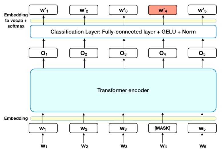
Exploring Machining Learning Techniques for
Text-Based Industry Classification
Haocheng Gao* Junjie He Kan Chen
June 2020
Abstract
This project aims to develop an effective machine learning text-based industry classi-
fication. We explore the use of various word embedding schemes and clustering algo-
rithms for industry classification. BERT, word2vec, doc2vec, latent semantic indexing
are used for word embedding, while greedy cosine-similarity, k-means, Gaussian mix-
ture model, and deep embedding for clustering are used as clustering algorithms. We
present our results for the companies listed in the US and Chinese markets.
Keywords: Text-based industry classification, BERT, word2vec, doc2vec, latent se-
mantic indexing, cosine similarity, k-means, Gausian mixture model, deep embedding
for clustering
* RiskManagement Institute, National University of Singapore
RiskManagement Institute, National University of Singapore
Risk Management Institute and Department of Mathematics, National University of Singapore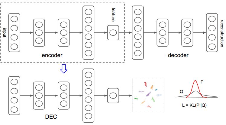
1     Introduction

    Recent advances in textual analysis and machine learning have enabled us to extract
useful information from company earnings reports, earnings conference call transcripts, and
firm-specific news inflows. Such information is often absent or incomplete in traditional
quantitative numerical data. Machine learning-based textual analysis has played an ever-
increasing role in finance and accounting research. One of the best examples for this type of
research was textual analysis in accounting research pioneered by Feng Li [1], who was able
to relate a company’s annual report readability (using a computational linguistic measure)
with its current earnings and earnings persistence. Another influential research has been
initiated by Hoberg and Phillips [2], who built a text-based network industry classification
of companies based on the similarity of their products and services. The database was built
for listed companies in the US using the business description section from 10-K annual filings;
it has become a widely used resource for many researchers.
    Given the rapid development in machine learning techniques for textual analysis, it is
desirable to investigate the use of these advanced techniques for finance research. In this
study, we explore their application to text-based industry classification. We investigate a
range of techniques used in word embedding schemes and clustering algorithms to gain intu-
ition on the usefulness of the techniques for text-based industry classification. An effective
machine learning-based industry classification scheme will not only complement the existing
industry classification but can also be used to classify new companies and unlisted private
companies, the standard classification of which might not be available.
    The outline of this report is as follows. We first introduce the commonly used and
recently developed textual analysis and clustering techniques. We then present the results
of text-based industry classification using these techniques for listed companies in the US
and the Chinese markets. We use several qualitative measures to evaluate the classification
obtained. We conclude by proposing some directions for future work.

                                              1
2        The Embedding Models

    The first step of textual analysis is to obtain the text embedding matrix. Our corpus is
the text containing the company descriptions. We use the company description for Chinese
listed companies from the China Securities Regulatory Commission (CSRC) and US-listed
companies from yahoo.com. We have also tried short company descriptions from Bloomberg1 .
The embedding models we have tried range from a bag of words to recently developed
BERT. In the following, we introduce the embedding methods that we find suitable for our
application.

2.1        Non-Machine Learning Methods

2.1.1       Bag of Words

    Bag of words is a representation of text that describes the occurrence of words in a
sentence or document. It maps each sentence to a vector consisting of counts of the individual
words used in the sentence. For example, we have two sentences: “Here are a white cat and a
black cat” and “Here is a dog”. The set of words used here are Here, are, is, a, white, black,
cat, dog. The bag of words vector representation of these two sentences are [1,1,0,2,1,1,2,0]
and [1,0,1,1,0,0,0,1].
    For our study of Chinese companies, there are 3924 documents in our corpus. The
business description is in Chinese, so we need to do a bit of preprocessing. We use Jieba
to cut words, and use Baidu stop word list to filter words. We then keep only those words
which occur more than 5 times in the corpus and contain in no more than 80% documents.
In total there are 1737 different words selected. This means that the size of the bag of words
matrix is (3789, 1737).
    For our study of US companies, we focus on the current Russell 3000 stocks and obtain
2896 documents in our corpus. We use NLTK in Python to remove stop words. We remove
    1
        The description from Bloomberg is shorter than that from yahoo.com, but they deliver similar results.

                                                       2
words that occur less than 5 times and in more than 80% of all business descriptions, and
we don’t use POS tagging. To compare with the result obtained by Hoberg and Phillips, we
also replicated their word selection criterion, which is a bit different from what we use here2 .
We get 4177 words using Hoberg and Phillips method and 4944 words using our methods.
2.1.2 TFIDF
Bag of words is very intuitive and easy to implement. But all words are equally weighted,
which is not preferable. To improve Bag of words one can add a numerical statistic to a word
to reflect how important a word is to a document. Tf-idf( Term frequency–inverse document
frequency) is one of such approaches. Tf-idf statistic is calculated as follow,
ft,d
tf (t, d) = P
t0 ∈d ft ,d
0
N
idf (t, D) = log
1 + {d ∈ D : t ∈ d}
tfidf (t, d, D) = tf × idf
where t is the term or word; d is the sentence or document; f is the frequency; D is the corpus;
N is the number of document in the corpus. The tf–idf value increases proportionally to the
number of times a word appears in the document and is offset by the number of documents
in the corpus that contain the word; this is to adjust for the fact that some words simply
appear more frequently in general. The resulting word matrix is obtained by putting the
tf-idf values to the corresponding locations in the bag of word matrix.
2.1.3 Latent semantic indexing
Bag of words and tf-idf use the word count and the frequency of individual words; there
is no semantic relationship between words. Besides, both models have the curse of dimen-
sionality. If there are many words in the corpus, the matrix will be extremely large.
2
They only keep nouns that appear in no more than 25% of all descriptions.
3LSI( Latent semantic indexing) is the model that can overcome both problems. LSI
assumes that words that are close in meaning will occur in similar pieces of text. Technically
this is done in LSI using singular value decomposition (SVD). Suppose we have the word
embedding matrix Am,n from a bag of words or tf-idf, we perform SVD on the matrix,
T T
Am,n = Um,m Σm,n Vn,n ≈ Um,k Σk,k Vk,n ,
where k is the desired embedding dimension of the word vector. Um,k is the word embed-
ding matrix for m different words and Vk,n is the sentence vector or document vector for n
documents.
In our model, we use the tf-idf matrix discussed in the previous section as A, and try
various values of k ranging from 200 to 1100
2.2 Machine Learning Methods
In this section, we will briefly introduce machine learning methods for generating a suit-
able sentence vector for our dataset. We will focus on the implementation without going
into the details of the individual methodologies.
2.2.1 From NNLM to Doc2vec
Generally speaking, NNLM (Neural Network Language Model) is the first language model
in machine learning. NNLM is based on Markov chain and it attempts to predict the
conditional probability of unknown word given the sequence of the preceding words.
f (wt , wt−1 , wt−2 , ..., wt−n+1 ) = p(wt |w1t−1 ),
where n is the length of Markov chain, f is the probability of wt when wt−1 , ..., wt−n+1 are
given.
4The following is the structure of NNLM:
Input : Xn−1,V
P rojection layer : An−1,m = Xn−1,V CV,m
concatenate An−1,m → A(n−1)m
Hidden layer : YV = UV,h tanh(dh + Hh,(n−1)m A(n−1)m )
+WV,(n−1)m A(n−1)m + bV
Output layer : f = sof tmax(YV )
X is the one-hot matrix; V is the number of words in the corpus; WV,(n−1)m is an optional
term. In the third step, we can also use the sum or mean instead of concatenation, which
means An−1,m → Am , and the dimension of H and W needs to change correspondingly.
The cost function is the cross entropy. After training we get CV,m , which is the resulting
embedding matrix for the words in the corpus.[3]
This method is, however, very slow. From the hidden layer to the output layer one
needs to calculate softmax parameters for all the words in the corpus at every step, which is
very time-consuming. A commonly used alternative is word2vec [4], which can be efficiently
implemented. In word2vec the hidden layer is dropped and the focus is on the word vector.
There are two types of word2vec models: CBoW and skip-gram. In CBoW, we mask the
central word in a sequence of a fixed length (2c + 1), then use other words to predict the
masked word. In skip-gram, it is the other way around. We choose the central word in a
fixed-length sequence, then use the central word to predict the remaining words. Skip-gram
is better for infrequent words than CBOW but normally takes longer to train.
To boost the speed further, two important schemes are often adopted in training: hier-
archical softmax and negative sampling.
Hierarchical softmax: This scheme was introduced to reduce the computational cost in soft-
max calculation, which normally needed to perform on all words. Hierarchical softmax makes
5use of the binary tree structure and avoid the expensive softmax calculation on the entire
vocabulary used. The main steps of hierarchical softmax are as follows.
1. Generate a Huffman tree based on word frequencies
2. Define P (0) = σ(xTw θw ); P (1) = 1 − P (+), where P (0) is probability of turning to the
left node
3. dw is the path to arrive at xw (dw
j = 0 indicating turning left at the j
th
node and dw
j = 1
indicating turning right); lw is the depth of dw
Qlw 1−djw dj w
4. Maximize log( j=2 P (dw w
j |xw , θj−1 ) P (dw w
j |xw , θj−1 ) )
Negative sampling: The idea of negative sampling is based on the concept of noise contrastive
estimation; a good model should differentiate fake signals from the real one. Instead of
changing all of the weights each time, we randomly select a small number of “negative” words
together with the “positive” word to update the weights on; this increases computational
efficiency dramatically. The steps of the negative sampling in the context of word2vec can
be summarized as follows.
1. Divide interval [0,1] to 108 equal length unit segments D
Count(w)3/4
2. For each words in the corpus, set length w = P 3/4 . Assign a subinterval of
u∈vocab Count(u)
this length in [0,1] to represent the word w. The length of the subinterval corresponds
to the probability the word is selected.
3. In each iteration, randomly select neg segments from D, and get the corresponding
words
Qneg
4. Maximize log(σ(xTw θw0 ) i=1 (1 − σ(xTw θwi )))
In our implementation of CBoW, we use the mean of xi , i ∈ [0, 2c] as the initial xw . In
each iteration we use the same gradient to update all of 2c word vectors. For skip-gram we
use xw to update xi , i ∈ [0, 2c] with different gradients at each iteration.
6So far we only consider the mechanism of representing words in vectors. But for our
application, we are concerned with the documents and the document similarity measure.
We need document embedding.
One way to get document embedding is to add or average over the word embeddings of
all the words in a document. But this simplistic approach does not work well. A better
solution is to add a document feature when we are training the word2vec model. This leads
to the so-called doc2vec.[5] In word2vec, we roll the training window to traverse the corpus,
and after the training, we get the vector representations for different words. In word2doc,
we add another vector xdoc for each document, so at each iteration, we train xdoc together
2c other word vectors. After training xdoc is used as our document representation.
In our tests we set neg = 10, learning rate ranging from 1e−2 to 1e−4 . The size of the
embedding vector is chosen from 50 to 400. We use both PV-DM (distributional memory
extension of CBoW) and PV-DBOW (extension of skip-gram to include document feature)
word2doc models.
2.2.2 From Attention to BERT
Bidirectional Encoder Representations from Transformers (BERT) is a technique for NLP
pre-training developed by Google in 2018. Since its invention, BERT has achieved state-of-
the-art performance on several natural language understanding tasks. For our word embed-
ding, we also tried the BERT model. Below we will give a very short description of BERT
starting with the attention models [6]
Attention is one of the most influential ideas in the deep learning community. In the
context of the encoder-decoder model of machine translation, the use of attention mechanism
helps memorize long source sentences. Rather than building a single context vector out of
the encoder’s last hidden state (as in the traditional Seq2Seq model), attention helps to
create shortcuts between the context vector and the entire source input. The weights of
these shortcut connections are customizable for each output element.
7The attention mechanism is formulated as follows. Given the input (h1 , h2 , ...hT ), where
hi is the output of last layer (such as one-hot vector, hidden state of RNN and so on), and
st−1 , which is the state at time t − 1 in the next layer, we want to predict st :
1. Compute e~t = (a(st−1 , h1 ), a(st−1 , h2 ), ..., a(st−1 , hT )), where a is a operator. For
example, we can use a(st−1 , hi ) = sTt−1 hi , a(st−1 , hi ) = sTt−1 W hi or a(st−1 , hi ) =
v T tanh(W1 hi + W2 st−1 )
PT
2. Compute α~t = sof tmax(~
et ). Then get the context vector ct = j=1 αtj hj
3. Get the state at time t, st = f (st−1 , ct ), where f is the logic used in this layer
Effectively attention takes two sentences, turns them into a matrix where the words of
one sentence form the columns, and the words of another sentence form the rows, and then
it makes matches, identifying relevant context. The attention can also be formulated for the
words within a sentence. This is the concept of self-attention. For any given word, we seek
to quantify the context that the sentence supplies, and identify which other words supply the
most context concerning the word in question. Self-attention is normally formulated using
matrix representation.
Self Attention:
1. Get the input XT,k = (hT1 ; hT2 ; ...; hTT ), where hi is the vector used in the current layer
Q K V
2. Initialize Query matrix Wk,m , Key matrix Wk,m , and Value matrix Wk,n
Q K V
3. Calculate Query Q = XT,k Wk,m , Key K = XT,k Wk,m and Value V = XT,k Wk,n
T
4. Self Attention(Q, K, V )T,n = sof tmax( QK
√ )V
m
5. Forward to the next layer
Technically the difference between attention and self-attention is that in attention, Query
depends on the next layer.
8Q K
We can generalize one self-attention to several self-attentions by initializing many Wk,m ,Wk,m
V
and Wk,n . Then we concatenate these outputs by column, and multiply a matrix to get it
1 2 m
to the proper shape: Concat(VT,n , VT,n , .., VT,n )Wnm,n . This is referred to as multi-head
attention.
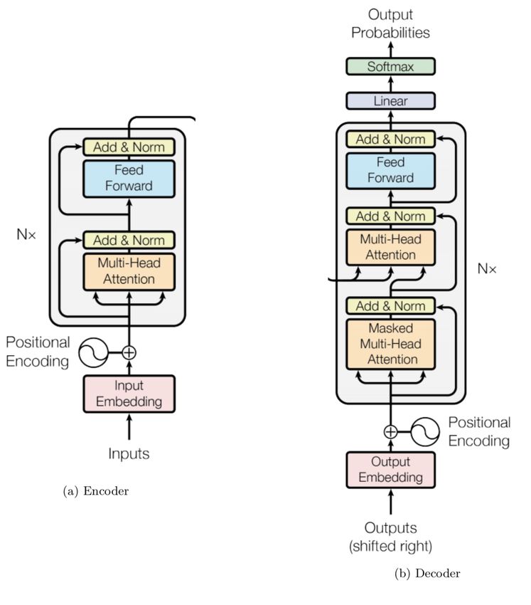
BERT[7] is considered to be the current state of the art language model for NLP. It
makes use of a transformer, which is an attention mechanism that learns contextual relations
between words in a text. A transformer used in the context of machine translation consists
of an encoder and a decoder. To generate word and document embedding, we are only
concerned with the encoder part, which is based on many multi-head attention layers, as
illustrated in Fig.3[7]. The structure of BERT is illustrated in Fig.4[7]. Instead of predicting
the next word in a sequence, BERT randomly masks words in the sentence and tries to predict
them. This means that the model looks in both directions and it uses the full context of
the sentence, both left, and right surroundings, to predict the masked word. There are two
choices of the model: a base model with a 12-layer encoder and a large model with a 24-layer
encoder. For our tests, we use the options RoBERTa-wwm-ext-large, Chinese for Chinese
descriptions and multi cased L-12 H-768 A-12 for English descriptions. We take CLS as the
document vector option and set the length as 512, which is the maximum input length of
BERT. For those documents longer than 512, we just average over the vectors generated
from different document parts.
3 The Clustering Algorithms
3.1 Greedy Clustering with Cosine Similarity
After obtaining the word/document embedding we can get a classification based on the
similarity of document embedding by employing a clustering algorithm. Holberg and Phillips
[2] used a bag of words as the embedding scheme and employed a greedy algorithm on a
cosine similarity measure. In this approach, we use document vectors (one for each company)
9Vi and Vj for a pair of firms i and j to calculate the firms’ pairwise similarity score as follows:
Company Cosine Similarity i,j = (Vi · Vj ) (1)
These form an N by N square matrix M (N is the number of companies considered).
The large number of words used in business descriptions ensures that the matrix M is not
sparse and that its entries are unrestricted real numbers in the interval [0, 1].
The greedy clustering algorithm works as follows. The industry classification is initialized
to have N industries, with each of the N firms residing within its one-firm industry. There
is a pairwise similarity for each pair of industries j and k, Ij,k . To reduce the industry count
to N-1, we take the maximum pairwise industry similarity
max Ij,k , (2)
j,k,j6=k
and combine two industries with the highest similarity. This process is repeated until the
number of industries reaches the desired number. When the two industries with mj and mk
firms are combined, all industry similarities relative to the new industry must be recomputed.
For a newly created industry, l, for example, its similarity with respect to an existing industry,
q is computed as the average firm pairwise similarity for all firm pairs in industries l and q
respectively:
mt Xmq
X Sx,y
Il,q = (3)
x=1 y=1
ml · mq
Here, Sx,y is the firm-level pairwise similarity between firm x in industry l and firm y in
industry q.
103.2 k-means
Another simple clustering algorithm is k-means clustering. The method aims to partition
n data points into k clusters in which each data point belongs to the cluster with the nearest
mean (cluster centers or cluster centroid), serving as a prototype of the cluster. Given a
set of data points {x1 , x2 , ..., xn }, where each data is represented by a d-dimensional real
vector, k-means clustering aims to partition the n data into k sets S = {S1 , S2 , ..., Sk } so as
to minimize the intra-cluster variance:
k X
X
arg min ||x − µi ||2 (4)
s
i=1 x∈Si
3.3 Deep Embedding for Clustering
The Deep Embedding for Clustering (DEC) model is built upon the Stacked Autoencoder
(SAE) model. Autoencoder is a kind of unsupervised learning structure that owns three
layers: an input layer, a hidden layer, and an output layer. The process of an autoencoder
training consists of two parts: encoder and decoder. The encoder is used for mapping the
input data into a hidden representation, and decoder is referred to as reconstructing input
data from the hidden representation. The SAEs are structured by stacking autoencoders
into hidden layers by an unsupervised layer-wise learning algorithm and then fine-tuned by
a supervised method. The structure of SAE is illustrated in Figure 5. After greedy layer-wise
training, we concatenate all encoder layers followed by all decoder layers, in reverse layer-wise
training order, to form a deep autoencoder and then fine-tune it to minimize reconstruction
loss. The final result is a multilayer deep autoencoder with a bottleneck coding layer in the
middle. We then discard the decoder layers and use the encoder layers as our initial mapping
between the data space and the feature space, as shown in Figure 6.[8]
Our implementation of DEC follows Xie et al. [9]. We add a new clustering layer
to iteratively refine the clusters by learning from their high confidence assignments with
the help of an auxiliary target distribution. The model is trained by matching the soft
11assignment to the target distribution. Kullback-Leibler (KL) divergence loss between the
soft assignments qi and the auxiliary distribution pi is used as the objective:
XX pij
L = KL(P ||Q) = pij log , (5)
i j
qij
where the soft assignments qi is defined (in the form of Student t-distribution) as
α+1
(1 + ||zi − µj ||2 /α)− 2
qij = P − α+1
. (6)
2
j 0 (1 + ||zi − µj 0 || /α)
2
Here zi is the embedding vector of company i, and uj is the centroid of group j. As in Ref.
[9], we set α = 1 and define the auxiliary distribution pi as:
qij2 /fj
pij = P 2
(7)
j 0 qij 0 /fj 0
The overall structure and the hyper-parameters are shown in Figure 7. The steps of the
training scheme are:
1. Pre-train the full SAE model and get the weights;
2. Pre-train a baseline machine learning classifier (we use k-means in this model);
3. Construct the DEC model and load the pre-train weights;
4. Initialize the clustering layer to the k-Means centroids;
5. Train the DEC model.
4 Data and Results
In this section we present our preliminary study, comparing our methods of industry
classification using different embedding schemes and clustering algorithms with the standard
industry classification. We choose GICS as our standard industry classification as it is
12available both for the US and Chinese markets. GICS is a common standard used by
many investors and fund managers and is shown to be a better classification than SIC
and NAICS for the US-listed companies [10]. In this report we use GICS at the industry
level (corresponding to the first 6 digits of GICS codes); there are 69 industries in total. For
comparison, we choose our clustering scheme to have about the same number of clusters.
For the US market, we also test the SIC classification scheme which was used for comparison
in Hoberg and Phillips.
For the US market, we use the stocks in the current Russell 3000 index with some stocks
that have a rather short price history removed. The stocks from the entire Chinese A-share
market (except those with short price histories) are included in our classification model for
the Chinese companies.
To evaluate industry classification we use two very different criteria. The first criterion
is based on the regression of the daily return series of each stock with the return of the
industry that the stock belongs to. Five-year daily returns are used. The average R2 from
the regressions (averaging over all the stocks in the universe) is used as a criterion to evaluate
the quality of the classification. The second criterion used is the across-industry variation
defined in Hoberg and Phillips. These criteria are also similar to the criteria used in Ref.
[10] for comparing industry classifications. The higher level of across-industry variation in
key firm characteristics indicates better informativeness of industry classification. The key
firm characteristics we use include Price/Book ratio, market beta, profit margin, ROA, and
ROE. To get more robust results we also remove some outliers, defined as at least 3 standard
deviations away of the overall mean (we use 5 standard deviations for the Chinese market).
The inter-industry variation of a firm characteristics is defined in terms of a weighted sum
qP
K (vm −vi )2
over all industries: σv = i=1 ni N
, where K is the number of industries, N is
the total number of firms, ni is the number of firms in industry i, vm is the overall mean
value of characteristics, and vi is the mean of the industry i. To simplify the presentation
we take the average of σv across all characteristics v considered. We found that σv for
13different characteristics follows a similar variation pattern with respect to the use of different
classification schemes, so the simplification of using the average does not affect the conclusion
we make regarding the informativeness of the classification.
We have tried different combinations of word/document embedding schemes and cluster-
ing algorithms. The results are presented in Table 1-4. We have tested Bag of Words, LSI,
PV-DBoW, PV-DM, and BERT as the embedding schemes, and k-means and DEC as the
algorithm for clustering. We use Tf-idf matrix for the input of LSI. For comparison, we also
list the result using Bag of Words and greedy clustering as was done in Hoberg and Philipps
and the result using the standard GICS classification.
For the US market, the use of the k-means clustering algorithm significantly improves the
performance of the classification scheme, both in terms of R2 and inter-industry variation.
In terms of word/document embedding schemes, LSI seems to work better than machine-
learning-based doc2vec and BERT. This indicates that for text-based industry classification,
the information related to the exact meaning of a sentence (which can be captured better
using ML-based methods) is not as important as the keywords and their distributions within
a document. As for the clustering algorithm, it turns out that a rather advanced technique,
DEC, is not as robust as the simple k-means algorithm. It generates in general a worse
classification when using the inter-industry variation measure (Table 2). Figures 1 and 2
plots the industry size distribution when k-means and DEC are used as clustering algorithms.
DEC gives rise to large size variability in the resulting industry classification with a few very
large industries and many small industries. Note that our use of LSI and k-means greatly
improve over the method used by Hoberg and Phillips (which is based on the combination
of the bag of words model and the greedy algorithm for clustering). In general, our best
text-based classification can match the informativeness of the GICS classification, indicating
that a text paragraph of company description contains most of the information needed for
good industry classification. We have also tried SIC and NAICS which were used in Hoberg
and Phillips for comparison. In general SIC and NAICS do not classify as well as GIC, and
14our best classification schemes give better classification in comparison using the two criteria
just discussed.
A similar conclusion can be drawn from our study of the Chinese market (Tables 3 and 4).
The best results are obtained with LSI (with the length of around 1000) as the embedding
scheme and k-means as the clustering algorithm.
5 Conclusion
We have explored the use of NLP and Machine learning techniques for our project of
text-based industry classification. We have constructed industry classification based on the
business description extracted from the profiles of the listed companies in the US and Chinese
markets. The study shows that the use of LSI as the word embedding scheme together with
the k-means clustering algorithm gives an industry classification that is comparable to the
standard GICS classification on the two informativeness measures we use. This indicates
that a business description of a moderate length (300 words on average) contains sufficient
information about companies’ business for good informative industry classification.
One of the potential applications of our classification method is to use the text-based
industry generated from the listed companies to classify unlisted companies that might not
have a proper standard classification. We only need to have a paragraph of the business
description of the company together with the LSI embedding matrix generated from the
descriptions of the listed companies to get its classification. The same approach can also be
applied to classify companies in a small market where the number of companies listed is too
small to directly use the text-based industry classification in that market.
For future research, we will explore how our machine learning-based method can be
improved with the aid of supervised learning of standard classification. We will also explore
the use of historical business descriptions to study the change of the industry classification
over time. Furthermore, we hope to apply the techniques presented in this paper to the
15more important problem of risk identification and decomposition using company news and
risk disclosures.
Tables
16Table 1: The average R2 for different combination of word/document embedding schemes
and clustering algorithms: US market(Russell 3000 companies)
Clustering Models
Embedding
standard greedy k-Means DEC
BERT / 0.4235 0.4353
Bag of Words 0.3602 0.4285 0.4034
PV-DM length 50 / 0.4430 0.4244
PV-DM length 100 / 0.4339 0.3792
PV-DM length 150 / 0.4481 0.3886
PV-DM length 200 / 0.4358 0.3981
PV-DM length 250 / 0.4391 0.4496
PV-DM length 300 / 0.4416 0.4280
PV-DM length 350 / 0.4369 0.4297
PV-DM length 400 / 0.4410 0.3770
PV-DBoW length 50 / 0.4332 0.4626
PV-DBoW length 100 / 0.4383 /
PV-DBoW length 150 / 0.4270 /
PV-DBoW length 200 0.4527 / 0.4299 0.4295
PV-DBoW length 250 / 0.4304 0.4371
PV-DBoW length 300 / 0.4276 0.4787
PV-DBoW length 350 / 0.4393 /
PV-DBoW length 400 / 0.4261 0.4538
LSI length 200 / 0.4537* 0.4962*
LSI length 300 / 0.4459 0.4768
LSI length 400 / 0.4421 0.4072
LSI length 500 / 0.4554 0.4244
LSI length 600 / 0.4362 0.4409
LSI length 700 / 0.4407 0.3842
LSI length 800 / 0.4417 0.4921
LSI length 900 / 0.4478 0.4005
LSI length 1000 / 0.4403 0.4068
LSI length 1100 / 0.4380 0.3933
*
The best results ever tested (excluding the result using GICS standard classification).
/
Combinations that did not generate meaningful results.
17Table 2: Inter-industry variation of firm characteristics for different combination of
word/document embedding schemes and clustering algorithms: US market(Russell 3000
companies)
Clustering Models
Embedding
standard greedy k-Means DEC
BERT / 0.5066 0.4897
Bag of Words 0.4143 0.5486* 0.3514
PV-DM length 50 / 0.4690 0.2920
PV-DM length 100 / 0.4569 0.3119
PV-DM length 150 / 0.4644 0.3534
PV-DM length 200 / 0.4644 0.3133
PV-DM length 250 / 0.4539 0.3053
PV-DM length 300 / 0.4538 0.2652
PV-DM length 350 / 0.4737 0.2836
PV-DM length 400 / 0.4731 0.3181
PV-DBoW length 50 / 0.4772 0.2582
PV-DBoW length 100 / 0.4801 0.2929
PV-DBoW length 150 / 0.4656 0.2689
PV-DBoW length 200 0.5555 / 0.4501 0.2770
PV-DBoW length 250 / 0.4552 0.2820
PV-DBoW length 300 / 0.4487 0.2617
PV-DBoW length 350 / 0.4446 0.2611
PV-DBoW length 400 / 0.4564 0.2741
LSI length 200 / 0.5091 0.3495
LSI length 300 / 0.5437 0.3608
LSI length 400 / 0.5469 0.3629
LSI length 500 / 0.5178 0.3817
LSI length 600 / 0.5249 0.4252
LSI length 700 / 0.5221 0.4026
LSI length 800 / 0.5374 0.3860
LSI length 900 / 0.5367 0.4039
LSI length 1000 / 0.5222 0.4006
LSI length 1100 / 0.5357 0.3544
*
The best results ever tested (excluding the result using GICS standard classification).
/
Combinations that did not generate meaningful results.
18Table 3: The average R2 for different combination of word/document embedding schemes
and clustering algorithms: Chinese market
Clustering Models
Embedding
standard greedy k-Means DEC
BERT / 0.4367 /
Bag of Words 0.4324 0.4482 0.3962
PV-DM length 50 / 0.4133 0.3916
PV-DM length 100 / 0.4173 0.3980
PV-DM length 150 / 0.4249 0.4010
PV-DM length 200 / 0.4217 0.4033
PV-DM length 250 / 0.4202 0.3990
PV-DM length 300 / 0.4225 0.4044
PV-DM length 350 / 0.4144 0.3941
PV-DM length 400 / 0.4172 0.4102
PV-DBoW length 50 / 0.4022 0.3849
PV-DBoW length 100 / 0.4023 /
PV-DBoW length 150 / 0.4063 /
PV-DBoW length 200 0.4535 / 0.4071 0.3979
PV-DBoW length 250 / 0.4031 0.3882
PV-DBoW length 300 / 0.4244 0.4038
PV-DBoW length 350 / 0.4084 0.4022
PV-DBoW length 400 / 0.4010 0.3748
LSI length 200 / 0.4445 0.4152
LSI length 300 / 0.4431 0.4162
LSI length 400 / 0.4345 0.4266
LSI length 500 / 0.4502 0.4356
LSI length 600 / 0.4484 0.4265
LSI length 700 / 0.4460 0.3938
LSI length 800 / 0.4410 0.4235
LSI length 900 / 0.4416 0.4023
LSI length 1000 / 0.4512* 0.4058
LSI length 1100 / 0.4423 0.4046
*
The best results ever tested (excluding the result using GICS standard classification).
/
Combinations that did not generate meaningful results.
19Table 4: Inter-industry variation of firm characteristics for different combination of
word/document embedding schemes and clustering algorithms: Chinese market
Clustering Models
Embedding
standard greedy k-Means DEC
BERT / 0.2273 /
Bag of Words 0.2287 0.2414 0.1044
PV-DM length 50 / 0.0791 0.1416
PV-DM length 100 / 0.1438 0.1189
PV-DM length 150 / 0.1419 0.1111
PV-DM length 200 / 0.1096 0.1209
PV-DM length 250 / 0.1254 0.0942
PV-DM length 300 / 0.1366 0.0957
PV-DM length 350 / 0.1379 0.0964
PV-DM length 400 / 0.1253 0.1000
PV-DBoW length 50 / 0.1111 0.0228
PV-DBoW length 100 / 0.1179 /
PV-DBoW length 150 / 0.1068 /
PV-DBoW length 200 0.2702 / 0.1235 0.1072
PV-DBoW length 250 / 0.1039 0.0928
PV-DBoW length 300 / 0.1123 0.1009
PV-DBoW length 350 / 0.1171 0.1052
PV-DBoW length 400 / 0.1176 0.0626
LSI length 200 / 0.2259 0.1151
LSI length 300 / 0.2258 0.1342
LSI length 400 / 0.2197 0.1229
LSI length 500 / 0.2136 0.1343
LSI length 600 / 0.2399 0.1363
LSI length 700 / 0.2365 0.1102
LSI length 800 / 0.2268 0.1248
LSI length 900 / 0.2405 0.1093
LSI length 1000 / 0.2292 0.0929
LSI length 1100 / 0.2443* 0.1246
*
The best results ever tested (excluding the result using GICS standard classification).
/
Combinations that did not generate meaningful results.
20Figures
Figure 1: Industry size distribution when using k-means as the clustering algorithm (the US
market)
21Figure 2: Industry size distribution when using DEC as the clustering algorithm (the US
market)
22Figure 3: Transformer structure from Ref. [6]
Figure 4: BERT output from Ref. [11]
23Figure 5: The Structure of a full SAE model, including encoder and decoder, from Ref. [12]
Figure 6: The Structure of an SAE model only considering encoder, from Ref. [9]
24Figure 7: The Structure of the DEC model
25References
[1] Feng Li. Annual report readability, current earnings, and earnings persistence. Journal
of Accounting & Economics, 45:221–247, 2008.
[2] Gerard Hoberg and Gordon M Phillips. Text-based network industries and endogenous
product differentiation. Journal of Political Economy, 124(5):1423–1465, 2016.
[3] Yoshua Bengio, Réjean Ducharme, Pascal Vincent, and Christian Jauvin. A neural
probabilistic language model. Journal of machine learning research, 3(Feb):1137–1155,
2003.
[4] Tomas Mikolov, Kai Chen, Greg Corrado, and Jeffrey Dean. Efficient estimation of
word representations in vector space. arXiv preprint arXiv:1301.3781, 2013.
[5] Quoc Le and Tomas Mikolov. Distributed representations of sentences and documents.
In International conference on machine learning, pages 1188–1196, 2014.
[6] Ashish Vaswani, Noam Shazeer, Niki Parmar, Jakob Uszkoreit, Llion Jones, Aidan N
Gomez, Lukasz Kaiser, and Illia Polosukhin. Attention is all you need. In Advances in
neural information processing systems, pages 5998–6008, 2017.
[7] Jacob Devlin, Ming-Wei Chang, Kenton Lee, and Kristina Toutanova. Bert: Pre-
training of deep bidirectional transformers for language understanding. arXiv preprint
arXiv:1810.04805, 2018.
[8] Jaime Zabalza, Jinchang Ren, Jiangbin Zheng, Huimin Zhao, Chunmei Qing, Zhijing
Yang, Peijun Du, and Stephen Marshall. Novel segmented stacked autoencoder for ef-
fective dimensionality reduction and feature extraction in hyperspectral imaging. Neu-
rocomputing, 185:1–10, 2016.
[9] Junyuan Xie, Ross Girshick, and Ali Farhadi. Unsupervised deep embedding for clus-
tering analysis. In Maria Florina Balcan and Kilian Q. Weinberger, editors, Proceedings
of The 33rd International Conference on Machine Learning, volume 48 of Proceedings
of Machine Learning Research, pages 478–487, New York, New York, USA, 20–22 Jun
2016. PMLR.
[10] Sanjeev Bhojraj, Charles M. C. Lee, and Derrek K. Oler. What’s my line? a comparison
of industry classification schemes for capital market research. Journal of Accounting
Research, 41(5):745–774, 2003.
[11] Rani Horev. Bert explained: State of the art language model for NLP.
https://towardsdatascience.com/bert-explained-state-of-the-art-language-model-
for-nlp-f8b21a9b6270. November 11, 2018.
[12] Arden Dertat. Applied deep learning - part 3: Autoencoders.
https://towardsdatascience.com/applied-deep-learning-part-3-autoencoders -
1c083af4d798. October 3, 2017.
26You can also read