Terabyte-scale Deep Multiple Instance Learning for Classification and Localization in Pathology
←
→
Page content transcription
If your browser does not render page correctly, please read the page content below
Terabyte-scale Deep Multiple Instance Learning
                                         for Classification and Localization in Pathology

                                         Gabriele Campanella1,2 , Vitor Werneck Krauss Silva1 , and Thomas J. Fuchs1,2
                                               1
                                                   Memorial Sloan Kettering Cancer Center, New York, NY 10065, USA
                                                        2
                                                           Weill Cornell Medicine, New York, NY 10065, USA
arXiv:1805.06983v1 [cs.CV] 17 May 2018

                                               Abstract. In the field of computational pathology, the use of decision
                                               support systems powered by state-of-the-art deep learning solutions has
                                               been hampered by the lack of large labeled datasets. Until recently, stud-
                                               ies relied on datasets in the order of few hundreds of slides which are not
                                               enough to train a model that can work at scale in the clinic. Here, we
                                               have gathered a dataset consisting of 12,160 slides, two orders of mag-
                                               nitude larger than previous datasets in pathology and equivalent to 25
                                               times the pixel count of the entire ImageNet dataset. Given the size
                                               of our dataset it is possible for us to train a deep learning model under
                                               the Multiple Instance Learning (MIL) assumption where only the overall
                                               slide diagnosis is necessary for training, avoiding all the expensive pixel-
                                               wise annotations that are usually part of supervised learning approaches.
                                               We test our framework on a complex task, that of prostate cancer di-
                                               agnosis on needle biopsies. We performed a thorough evaluation of the
                                               performance of our MIL pipeline under several conditions achieving an
                                               AUC of 0.98 on a held-out test set of 1,824 slides. These results open the
                                               way for training accurate diagnosis prediction models at scale, laying the
                                               foundation for decision support system deployment in the clinic.

                                         1   Introduction

                                         In recent years there has been a strong push towards the digitization of pathology
                                         with the birth of the new field of computational pathology [6,5]. The increasing
                                         size of available digital pathology data, coupled with the impressive advances
                                         that the fields of computer vision and machine learning have made in recent
                                         years, make for the perfect combination to deploy decision support systems in
                                         the clinic.
                                             Despite a few success stories, translating the achievements of computer vi-
                                         sion to the medical domain is still far from solved. The lack of large datasets
                                         which are indispensable to learn high capacity classification models has set back
                                         the advance of computational pathology. The “CAMELYON16” challenge for
                                         metastasis detection [4] contains one of the largest labeled datasets in the field
                                         with a total of 400 Whole Slide Images (WSIs). Such an amount of cases is
                                         extremely small compared to the millions of instances present in the ImageNet
                                         dataset [2]. One widely adopted solution to face the scarcity of labeled examples
                                         in pathology is to take advantage of the size of each example. Pathology slides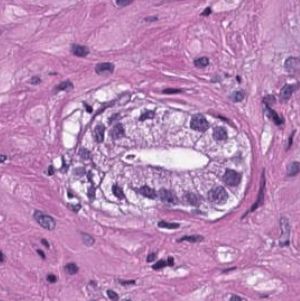
scanned at 20x magnification produce image files of several Giga-pixels. About
470 WSIs contain roughly the same number of pixels as the entire ImageNet
dataset. By breaking the WSIs into small tiles it is possible to obtain thousands
of instances per slide, enough to learn high-capacity models from a few hundred
slides. Pixel-level annotations for supervised learning are prohibitively expensive
and time consuming, especially in pathology. Some efforts along these lines [10]
have achieved state-of-the-art results on CAMELYON16. Despite the success on
these carefully crafted datasets, the performance of these models hardly transfers
to the real life scenario in the clinic because of the huge variance in real-world
samples that is not captured by these small datasets.
In summary, until now it was not possible to train high-capacity models
at scale due to the lack of large WSI datasets. Here we gathered a dataset of
unprecedented size in the field of computational pathology consisting of over
12,000 slides from prostate needle biopsies, two orders of magnitude larger than
most datasets in the field and with roughly the same number of pixels of 25
ImageNet datasets. Whole slide prostate cancer classification was chosen as a
representative one in computational pathology due to its medical relevance and
its computational difficulty. Prostate cancer is expected to be the leading source
of new cancer cases for men and the second most frequent cause of death behind
only the cancers of the lung [12], and multiple studies have shown that prostate
cancer diagnosis has a high inter- and intra-observer variability [19,13,7]. It is im-
portant to note that the classification is frequently based on the presence of very
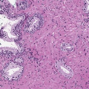
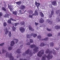
small lesions that can comprise just a fraction of 1% of the tissue surface. Figure
1 depicts the difficulty of the task, where only a few tumor glands concentrated
in a small region of the slide determine the diagnosis.
Since the introduction of the Multiple Instance Learning (MIL) framework
by [3] in 1997 there have been many efforts from both the theory and application
of MIL in the computer vision literature [1,14,17,18]. While the MIL framework
is very applicable to the case of WSI diagnosis and despite its success with classic
computer vision algorithms, MIL has been applied much less in computational
pathology (see Related Work) due to the lack of large WSI datasets. In this
work we take advantage of our large prostate needle biopsy dataset and propose
a Deep Multiple Instance Learning (MIL) framework where only the whole slide
class is needed to train a convolutional neural network capable of classifying
digital slides on a large scale.
2 Related work
This work is related to the extensive literature on computer vision applications
to hystopathology. In contrast to most of them, here we use weak supervision at
the WSI-level instead of strong supervision at the small tile-level. A few other
studies have also tackled medical image diagnosis tasks with weak supervision
under the MIL assumption: in [15] a convolutional neural network is used to
classify medical images; in [16] a MIL approach is combined with feature clus-
tering for classification and segmentation tasks. More recently, [9] showed how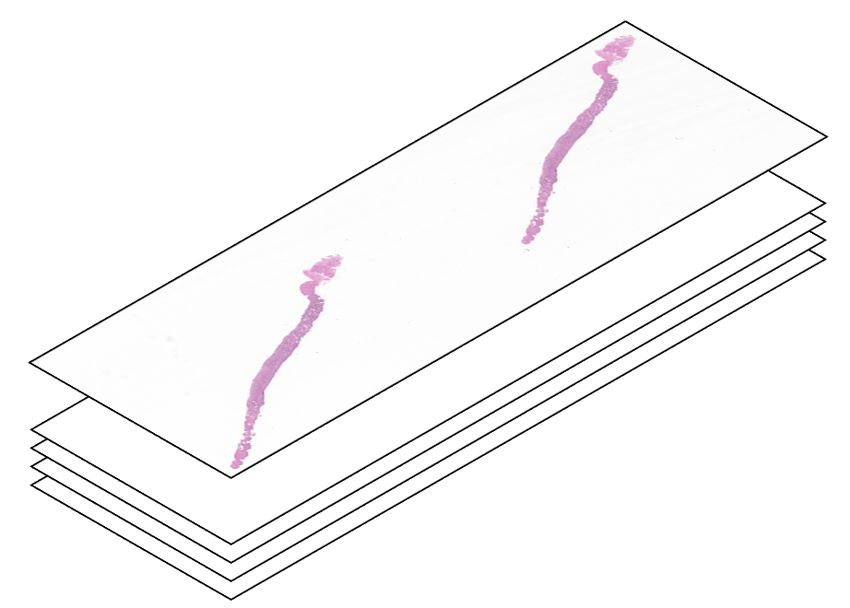
28,649 px

                  63,744 px               3,000 px         1,200 px          300 px

Fig. 1. Prostate cancer diagnosis is a difficult task. The diagnosis can be based
on very small lesions. In the slide above, only about 6 small tumor glands are present.
The right most image shows an example tumor gland. Its relation to the entire slide is
put in evidence to reiterate the complexity of the task.

learning a fusion model on top of a tile-level classifier trained with MIL can boost
performance on two tasks: glioma and non-small-cell lung carcinoma classifica-
tion. This work is considered the state-of-the-art in terms on weak supervision in
hystopathology images. All previous works used small datasets which precludes
a proper estimation of the clinical relevance of the models. What sets our efforts
apart from others is the scale of our datasets which can be considered clinically
relevant.

3           Dataset

Our dataset consists of 12,160 needle biopsies slides scanned at 20x magnifi-
cation, of which 2,424 are positive and 9,736 are negative. The diagnosis was
retrieved from the original pathology reports in the Laboratory Information
System (LIS) at MSKCC. As visualized in Figure 2, the dataset was randomly
split in training (70%), validation (15%) and testing (15%). No augmentation
was performed during training. For the “dataset size importance” experiments,
explained further in the Experiments section, a set of slides from the above
mentioned training set were drawn to create training sets of different sizes.

4           Methods

Classification of a whole digital slide based on a tile-level classifier can be for-
malized under the classic MIL paradigm when only the slide-level class is known
and the classes of each tile in the slide are unknown. Each slide si from our slide
pool S = {si : i = 1, 2, ..., n} can be considered as a bag consisting of a multitude
of instances (tiles). For positive bags, there must exist at least one instance that
is classified as positive by some classifier. For negative bags instead, all instances
must be classified as negative. Given a bag, all instances are exhaustively clas-
sified and ranked according to their probability of being positive. If the bag is
positive, the top-ranked instance should have a probability of being positive that
approaches one, while if it is negative, the probability should approach zero. The
complete pipeline of our method comprises the following steps: (i) tiling of each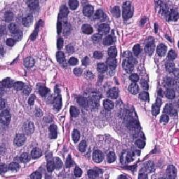
Dataset Size Experiments                      Shuffled Slides   All Other Experiments
                                                   1
                                                   2
                                         100       3
                                   200             4
                             500                   5
                                                   6
                                                   7
                         1,000                     8

                     2,000                                                  Training Set
                                                                            8,512
                4,000
             6,000
                     Training Sets
             8,000

                     Validation Set                                         Validation Set
                                 2,000                                      1,824

                                                                            Held-out Test Set
                                                                            1,824
                                               12,160

Fig. 2. Prostate needle biopsy dataset split. The full dataset was divided into
70-15-15% splits for training, validation, and test for all experiments except the ones
investigating dataset size importance. For those, out of the 85% training/validation
split of the full dataset, training sets of increasing size were generated along with a
common validation set.

slide in the dataset; for each epoch, which consists of an entire pass through the
training data, (ii) a complete inference pass through all the data; (iii) intra-slide
ranking of instances; (iv) model learning based on the top-1 ranked instance for
each slide. A schematic of the method is shown in Figure 3.

Slide Tiling: We generate the instances for each slide by tiling it on a grid.
All the background tiles are efficiently discarded by our algorithm, reducing
drastically the amount of computation per slide, since quite a big portion of
it is not covered by tissue. Furthermore, tiling can be performed at different
magnification levels and with various levels of overlap between adjacent tiles. In
this work we investigated three magnification levels (5x, 10x and 20x), with no
overlap for 10x and 20x magnification and with 50% overlap for 5x magnification.
On average each slide contains about 100 non overlapping tissue tiles at 5x
magnification and 1,000 at 20x magnification. Given a tiling strategy we produce
our bags B = {Bsi : i = 1, 2, ..., n} where Bsi = {bi,1 , bi,2 , ..., bi,m } is the bag for
slide si containing m total tiles. An example of tiling can be seen in Figure A.1.

Model Training: The model is a function fθ with current parameters θ that
maps input tiles bi,j to class probabilities for “negative” and “positive” classes.
Given our bags B we obtain a list of vectors O = {oi : i = 1, 2, ..., n} one
for each slide si containing the probabilities of class “positive” for each tile
bi,j : j = 1, 2, ..., m in Bsi . We then obtain the index ki of the tile within each
slide which shows the highest probability of being “positive” ki = argmax(oi ).
The highest ranking tile in bag Bsi is then bi,k . The output of the network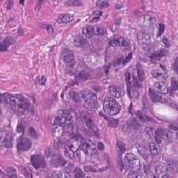
Ranked
                                                                                                   Instances
                                        Bag
                                                                                                               Cross-entropy
                                                                                                                   Loss

                                                                               Tumor Probability
Bags

                                                                     Model
                                        Instances
                                                                   Inference
                                                                                                                  Model
Labels      0, 1, 1, 0, 0, 0, ...                          ...                                                   Learning

Fig. 3. Schematic of the MIL pipeline. The slide or bag consists of multiple in-
stances. Given the current model, all the instances in the bag are used for inference.
They are then ranked according to the probability of being of class positive (tumor
probability). The top ranked instance is used for model learning via the standard cross-
entropy loss.

ỹi = fθ (bi,k ) can be compared to yi , the target of slide si , thorough the cross-
entropy loss l as in Equation 1.

                             l = −w1 [yi log(ỹi )] − w0 [(1 − yi ) log(1 − ỹi )]                                          (1)

Given the unbalanced frequency of classes, weights w0 and w1 , for negative
and positive classes respectively, can be used to give more importance to the
underrepresented examples. The final loss is the weighted average of the losses
over a mini-batch. Minimization of the loss is achieved via stochastic gradient
descent using the Adam optimizer and learning rate 0.0001. We use mini-batches
of size 512 for AlexNet, 256 for ResNets and 128 for VGGs.

Model Testing: At test time all the instances of each slide are fed through
the network. Given a threshold (usually 0.5), if at least one instance is positive
then the entire slide is called positive; if all the instances are negative then the
slide is negative. Accuracy, confusion matrix and ROC curve are calculated to
analyze performance.

5        Experiments
Hardware and Software: We run all the experiments in our in-house HPC
cluster. In particular we took advantage of 7 NVIDIA DGX-1 workstations each
containing 8 V100 Volta GPUs. We used OpenSlide [8] to access on-the-fly the
WSI files and PyTorch [11] for data loading, building models, and training.
Further data manipulation of results was performed in R.

Weight Tuning: Needle biopsy diagnosis is an unbalanced classification task.
Our full dataset consists of 19.9% positive examples and 80.1% negative ones.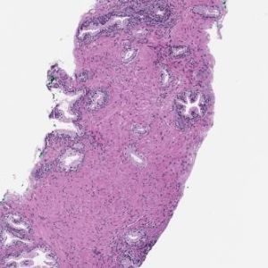
To determine whether weighting the classification loss is beneficial, we trained
on the full dataset an AlexNet and a Resnet18 networks, both pretrained on
ImageNet, with weights for the positive class w1 equal to 0.5, 0.7, 0.9, 0.95 and
0.99. The weights for both classes sum to 1, where w1 = 0.5 means that both
classes are equally weighted. Each experiment was run five times and the best
validation balanced error for each run was gathered. Training curves and vali-
dation balanced errors are reported in Figure B.1. We determined that weights
0.9 and 0.95 gave the best results. For the reminder of the experiments we used
w1 = 0.9.

Dataset Size Importance: In the following set of experiments we determine
how dataset size affects performance of a MIL based slide diagnosis task. For
these experiments the full dataset was split in a common validation set with
2,000 slides and training sets of different sizes: 100, 200, 500, 1,000, 2,000, 4,000,
6,000. Each bigger training dataset fully contained all previous datasets. For
each condition we trained an AlexNet five times and the best balanced errors
on the common validation set are shown in Figure 4 demonstrating how a MIL
based classifier could not have been trained until now due to the lack of a large
WSI dataset. Training curves and validation errors are also reported in Figure
C.1.
          Minimum Balanced Validation Error

                                              0.5   ●
                                                      ●
                                                    ●●    ●           ●
                                                              ●
                                                     ●        ●
                                                                      ●●    ●
                                                                      ●
                                                          ●

                                              0.4
                                                          ●                  ●

                                                                      ●                ●
                                                                            ●
                                              0.3                           ●
                                                                             ●
                                                                                   ●

                                                                                    ●
                                                                                   ●
                                                                                  ●
                                              0.2                                          ●●
                                                                                           ● ●
                                                                                                 ●
                                                                                                  ●●● ●
                                                                                                   ● ●●
                                                                                                       ●●

                                                    102                     103                         104
                                                                  Dataset Size (# WSIs)

Fig. 4. Importance of dataset size for MIL classification performance. Train-
ing was performed for datasets of increasing size. The experiment underlies the fact
that a large number of slides is necessary for generalization of learning under the MIL
setup.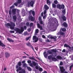
Model comparison: We tested various standard image classification models
pretrained on ImageNet (AlexNet, VGG11-BN, ResNet18, Resnet34) under the
MIL setup at 20x magnification. Each experiment was run for up to 60 epochs
for at least five times with different random initializations of the classification
layers. In terms of balanced error on the validation set, AlexNet performed the
worst, followed by the 18-layer ResNet and the 34-layer ResNet. Interestingly,
the VGG11 network achieved results similar to those of the ResNet34 on this
task. Training and validation results are reported in Figure D.1.

Test Dataset Performance: For each architecture, the best model on the vali-
dation dataset was chosen for final testing. Performance was similar with the
one on the validation data indicating good generalization. The best models were
Resnet34 and VGG11-BN which achieved 0.976 and 0.977 AUC respectively.
The ROC curves are shown in Figure 6a.

Error Analysis: A thorough analysis of the error modalities of the VGG11-BN
model was performed with the help of an expert pathologist. Of the 1,824 test
slides, 55 were false positives (3.7% false positive rate) and 33 were false nega-
tives (9.4% false negative rate). The analysis of the false positives found seven
cases that were considered highly suspicious for prostate cancer. Six cases were
considered “atypical”, meaning that following-up with staining would have been
necessary. Of the remaining false positives, 18 were a mix of known mimickers of
prostate cancer: adenosis, atrophy, benign prostatic hyperplasia, and inflamma-
tion. The false negative cases were carefully inspected, but in six cases no sign
of prostate cancer was found by the pathologist. The rest of the false negative
cases were characterized by very low volume of cancer tissue.

Feature Embedding Visualization: Understanding what features the model uses
to classify a tile is an important bottle-neck of current clinical applications of
deep learning. One can gain insight by visualizing a projection of the feature
space in two dimensions using dimensionality reduction techniques such as PCA.
We sampled 50 tiles from each test slide, in addition to its top-ranked tile,
and extracted the final feature embedding before the classification layer. As an
example, we show the results of the ResNet34 model in Figure 5. From the 2D
projection we can see a clear decision boundary between positively and negatively
classified tiles. Interestingly, most of the points are clustered at the top left region
where we have tiles that are rarely top-ranked in a slide. By observing examples
in this region of the PCA space we can determine they are tiles containing
stroma. Tiles containing glands extend along the second principal component
axis, where there is a clear separation between benign and malignant glands.
Other top-ranked tiles in negative slides contain edges and inked regions. The
model trained only with the weak MIL assumption was still able to extract
features that embed visually and semantically related tiles close to each other.

Augmentation Experiments: We also ran a small experiment with a ResNet34
model to determine whether augmentation of the data with rotations and flips
Other
Benign Glands

                                                  Stroma
Malignant Glands

                       PC2

                                    PC1

 Fig. 5. Visualization of the feature space with PCA. A ResNet34 model trained
 at 20x was used to obtain the feature embedding right before the final classification
 layer for a random set of tiles in the test set. The embedding was reduced to two
 dimensions with PCA and plotted. Non-gray points are the top-ranked tiles coming
 from negative and positive slides. Tiles corresponding to points in the scatter plot are
 sampled from different regions of the 2D PCA embedding.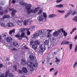
during training could help lower the generalization error. The results, presented
in Figure E.1, showed no indication of a gain in accuracy when using augmen-
tation.

Magnification comparison: We then trained VGG11-BN and ResNet34 mod-
els with tiles generated at 5x and 10x magnifications. Lowering the magnification
led consistently to higher error rates across both models. Training curves and
validation errors are shown in Figure F.1. We also generated ensemble models
by averaging or taking the maximum response across different combinations of
the three models trained at different magnifications. On the test set these naive
multi-scale models outperformed the single-scale models, as can be seen in the
ROC curves in Figure 6b. In particular, max-pooling the response of all the three
models resulted in the best results with an AUC of 0.979, a balanced error of
5.8% and a false negative rate of 4.8%.

a)                                                                           b)
                          1.00                                                                         1.00

                          0.75                                                                         0.75
     True Positive Rate

                                                                                  True Positive Rate

                          0.50                                                                         0.50
                                        Model                                                                           Model
                                            VGG11−BN 20x (AUC: 0.977)                                                       Ensemble (AUC: 0.9793)

                          0.25                  ResNet34 20x (AUC: 0.976)                              0.25                      20x (AUC: 0.9757)
                                                ResNet18 20x (AUC: 0.955)                                                        10x (AUC: 0.9717)
                                                 AlexNet 20x (AUC: 0.925)                                                           5x (AUC: 0.9709)
                          0.00                                                                         0.00
                                 0.00    0.25       0.50     0.75     1.00                                    0.00   0.25    0.50       0.75     1.00
                                         False Positive Rate                                                         False Positive Rate

Fig. 6. Test set ROC curves. a) Results of the model comparison experiments on the
test set. ResNet34 and VGG11-BN models achieved the best performance. b) Results of
the magnification comparison experiments for a ResNet34 model. Lower magnifications
lead to worse performance. The max-pooling ensemble model achieves the best result
in our experiments.

6     Conclusions

In this study we have analyzed in depth the performance of convolutional neural
networks under the MIL assumption for WSI diagnosis. We focused on needle
biopsies of the prostate as a complex representative task and obtained the largest
dataset in the field with 12,160 WSIs. We demonstrated how it is possible to train
high-performing models for WSI diagnosis only using the slide-level diagnosis and
no further expert annotation using the standard MIL assumption. We showed
that final performance greatly depends on the dataset size. Our best model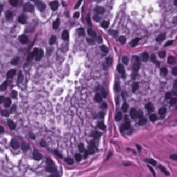
achieved an AUC of 0.98 and a false negative rate of 4.8% on a held-out test set
consisting of 1,824 slides. We argue that given the current efforts in digitizing the
pathology work-flow, approaches like ours can be extremely effective in building
decision support systems that can be effectively deployed in the clinic.

References
 1. Stuart Andrews, Thomas Hofmann, and Ioannis Tsochantaridis. Multiple instance
    learning with generalized support vector machines. In AAAI/IAAI, pages 943–944,
    2002.
 2. Jia Deng, Wei Dong, Richard Socher, Li-Jia Li, Kai Li, and Li Fei-Fei. Imagenet:
    A large-scale hierarchical image database. In Computer Vision and Pattern Recog-
    nition, 2009. CVPR 2009. IEEE Conference on, pages 248–255. IEEE, 2009.
 3. Thomas G. Dietterich, Richard H. Lathrop, and Tomás Lozano-Pérez. Solving the
    multiple instance problem with axis-parallel rectangles. 89(1):31–71.
 4. Babak Ehteshami Bejnordi, Mitko Veta, Paul Johannes van Diest, Bram van Gin-
    neken, Nico Karssemeijer, Geert Litjens, Jeroen A. W. M. van der Laak, and
    the CAMELYON16 Consortium, Meyke Hermsen, Quirine F Manson, Maschenka
    Balkenhol, Oscar Geessink, Nikolaos Stathonikos, Marcory CRF van Dijk, Peter
    Bult, Francisco Beca, Andrew H Beck, Dayong Wang, Aditya Khosla, Rishab
    Gargeya, Humayun Irshad, Aoxiao Zhong, Qi Dou, Quanzheng Li, Hao Chen,
    Huang-Jing Lin, Pheng-Ann Heng, Christian Haß, Elia Bruni, Quincy Wong, Ugur
    Halici, Mustafa Ümit Öner, Rengul Cetin-Atalay, Matt Berseth, Vitali Khvatkov,
    Alexei Vylegzhanin, Oren Kraus, Muhammad Shaban, Nasir Rajpoot, Ruqayya
    Awan, Korsuk Sirinukunwattana, Talha Qaiser, Yee-Wah Tsang, David Tellez,
    Jonas Annuscheit, Peter Hufnagl, Mira Valkonen, Kimmo Kartasalo, Leena Lato-
    nen, Pekka Ruusuvuori, Kaisa Liimatainen, Shadi Albarqouni, Bharti Mungal, Ami
    George, Stefanie Demirci, Nassir Navab, Seiryo Watanabe, Shigeto Seno, Yoichi
    Takenaka, Hideo Matsuda, Hady Ahmady Phoulady, Vassili Kovalev, Alexander
    Kalinovsky, Vitali Liauchuk, Gloria Bueno, M. Milagro Fernandez-Carrobles, Is-
    mael Serrano, Oscar Deniz, Daniel Racoceanu, and Rui Venâncio. Diagnostic as-
    sessment of deep learning algorithms for detection of lymph node metastases in
    women with breast cancer. 318(22):2199.
 5. Thomas J. Fuchs and Joachim M. Buhmann. Computational pathology: Challenges
    and promises for tissue analysis. 35(7):515–530.
 6. Thomas J. Fuchs, Peter J. Wild, Holger Moch, and Joachim M. Buhmann. Com-
    putational pathology analysis of tissue microarrays predicts survival of renal clear
    cell carcinoma patients. In Proceedings of the international conference on Medical
    Image Computing and Computer-Assisted Intervention MICCAI, volume 5242 of
    Lecture Notes in Computer Science, pages 1–8. Springer-Verlag.
 7. Donald F. Gleason. Histologic grading of prostate cancer: a perspective. 23(3):273–
    279.
 8. Adam. Goode, Benjamin. Gilbert, Jan. Harkes, Drazen. Jukic, and Mahadev.
    Satyanarayanan. OpenSlide: A vendor-neutral software foundation for digital
    pathology. Journal of Pathology Informatics, 4(1):27, 2013.
 9. Le Hou, Dimitris Samaras, Tahsin M. Kurc, Yi Gao, James E. Davis, and Joel H.
    Saltz. Patch-based convolutional neural network for whole slide tissue image clas-
    sification. In Proceedings of the IEEE Conference on Computer Vision and Pattern
    Recognition, pages 2424–2433.
10. Yun Liu, Krishna Gadepalli, Mohammad Norouzi, George E. Dahl, Timo
Kohlberger, Aleksey Boyko, Subhashini Venugopalan, Aleksei Timofeev, Philip Q.
Nelson, and Greg S. Corrado. Detecting cancer metastases on gigapixel pathology
images.
11. Adam Paszke, Sam Gross, Soumith Chintala, Gregory Chanan, Edward Yang,
Zachary DeVito, Zeming Lin, Alban Desmaison, Luca Antiga, and Adam Lerer.
Automatic differentiation in pytorch. 2017.
12. Rebecca L. Siegel, Kimberly D. Miller, and Ahmedin Jemal. Cancer statistics,
2016: Cancer statistics, 2016. 66(1):7–30.
13. Hans Svanholm and Henrik Mygind. Prostatic carcinoma reproducibility of histo-
logic grading. APMIS, 93(1-6):67–71, 1985.
14. Nakul Verma. Learning from data with low intrinsic dimension. University of
California, San Diego.
15. Yan Xu, Tao Mo, Qiwei Feng, Peilin Zhong, Maode Lai, and Eric I-Chao Chang.
Deep learning of feature representation with multiple instance learning for medical
image analysis. pages 1626–1630. IEEE.
16. Yan Xu, Jun-Yan Zhu, Eric I-Chao Chang, Maode Lai, and Zhuowen Tu. Weakly
supervised histopathology cancer image segmentation and classification. 18(3):591–
604.
17. Cha Zhang, John C Platt, and Paul A Viola. Multiple instance boosting for object
detection. In Advances in neural information processing systems, pages 1417–1424,
2006.
18. Qi Zhang and Sally A Goldman. Em-dd: An improved multiple-instance learning
technique. In Advances in neural information processing systems, pages 1073–1080,
2002.
19. Şükrü O. Özdamar, Şaban Sarikaya, Levent Yildiz, M. Kemal Atilla, Bedrİ Kan-
demir, and Sacİt Yildiz. Intraobserver and interobserver reproducibility of WHO
and gleason histologic grading systems in prostatic adenocarcinomas. 28(1):73–77.A Slide Tiling
20x
10x
5x
Fig. A.1. An example of a slide tiled on a grid with no overlap at different magnifi-
cations. The slide is the bag and the tiles constitute the instances of the bag. In this
work instances at different magnifications are not part of the same bag.B Weight Tuning
a)
0.5 0.7 0.9 0.95 0.99
0.8
0.6
AlexNet
Cross−entropy Loss
0.4
0.2
0.0
0.8
0.6
ResNet18
0.4
0.2
0.0
0 10 20 30 40 0 10 20 30 40 0 10 20 30 40 0 10 20 30 40 0 10 20 30 40
Epoch
b)
0.5 0.7 0.9 0.95 0.99
0.5
0.4
Balanced Validation Error
AlexNet
0.3
0.2
0.1
0.5
0.4
ResNet18
0.3
0.2
0.1
0 10 20 30 40 0 10 20 30 40 0 10 20 30 40 0 10 20 30 40 0 10 20 30 40
Epoch
c)
AlexNet ResNet18
Minimum Balanced Validation Error
●
0.175
●
●
●● ●
●
●
●
0.150 ●
●
● ● ●
●● ●●●
● ●
●
●●
● ●
0.125
●
●
● ●
●●
●
0.100 ●●
●
●
0.5 0.7 0.9 0.95 0.99 0.5 0.7 0.9 0.95 0.99
Positive Class Weight
Fig. B.1. Tuning the class weight for the cross-entropy loss. Different positive
class weights were tested: 0.5 (balanced weight), 0.7, 0.9, 0.95, 0.99. Each experiment
was run 5 times. a) Training curves with cross-entropy loss. b) Balanced error rates on
the validation set. c) For each weight the minimum achieved error was gathered. We
chose a value of 0.9 for all subsequent experiments.C Dataset Size
a)
100 200 500 1000 2000
1.5
1.0
Cross−entropy Loss
0.5
0.0
0 10 20 30 40 0 10 20 30 40
4000 6000 8000
1.5
1.0
0.5
0.0
0 10 20 30 40 0 10 20 30 40 0 10 20 30 40
Epoch
b)
100 200 500 1000 2000
0.5
Balanced Validation Error
0.4
0.3
0.2
0 10 20 30 40 0 10 20 30 40
4000 6000 8000
0.5
0.4
0.3
0.2
0 10 20 30 40 0 10 20 30 40 0 10 20 30 40
Epoch
Fig. C.1. Training and validation curves for the dataset size experiments.
Good generalization error on the validation set requires a large number of training
WSIs. a) Training curves with cross-entropy loss. b) Balanced error rates on the vali-
dation set.D Model Comparison
a)
AlexNet VGG11−BN ResNet18 ResNet34
Cross−entropy Loss
0.6
0.4
0.2
0.0
0 20 40 60 0 20 40 60 0 20 40 60 0 20 40 60
Epoch
b)
AlexNet VGG11−BN ResNet18 ResNet34
0.5
Balanced Validation Error
0.4
0.3
0.2
0.1
0 20 40 60 0 20 40 60 0 20 40 60 0 20 40 60
Epoch
c)
Minimum Balanced Validation Error
●
●● ●
●
0.125
● ●
●●
●
●●
0.100 ● ●
●
●
●
●● ●
0.075 ●●
●
● ● ●
● ●
●
●
AlexNet VGG11−BN ResNet18 ResNet34
Models
Fig. D.1. Comparison of various standard CNN architectures on the MIL
task at 20x magnification. AlexNet, VGG11 with batch-normalization, ResNet18
and ResNet34 models were trained five times each for up to 60 epochs. a) Training
curves with cross-entropy loss. b) Balanced error rates on the validation set. c) For
each model, the minimum achieved error was gathered.E Augmentation Experiments
a) b)
Augmented Not Augmented Augmented Not Augmented
0.5
Balanced Validation Error
0.6
Cross−entropy Loss
0.4
0.4 0.3
0.2 0.2
0.1
0.0
0 20 40 60 0 20 40 60 0 20 40 60 0 20 40 60
Epoch Epoch
c)
Minimum Balanced Validation Error
●
0.085
●
●
0.080
●
● ● ●
0.075 ●
●
0.070 ●
0.065 ●
Augmented Not Augmented
Fig. E.1. Comparison of models trained at 20x magnification with and with-
out augmentation. A ResNet34 model was trained with augmentation consisting of
flips and rotations, and without augmentation. Augmentation does not improve gen-
eralization. a) Training curves with cross-entropy loss. b) Balanced error rates on the
validation set. c) For each model, the minimum achieved error was gathered.F Magnification Comparisons
a)
5x 10x 20x
0.6
ResNet34
0.4
Cross−entropy Loss
0.2
0.0
0.6
VGG11−BN
0.4
0.2
0.0
0 20 40 60 0 20 40 60 0 20 40 60
Epoch
b)
5x 10x 20x
0.5
0.4
Balanced Validation Error
ResNet34
0.3
0.2
0.1
0.5
0.4
VGG11−BN
0.3
0.2
0.1
0 20 40 60 0 20 40 60 0 20 40 60
Epoch
c)
Minimum Balanced Validation Error
●
●
0.09
●
●
● ● ●
0.08
●
● ●
Model
●
●
●
●
● ResNet34
● ●
●
●●
●
●
●
●
● ● VGG11−BN
●
0.07 ●●
●
●
●
● ● ●
●
●
0.06
5x 10x 20x
Magnification
Fig. F.1. Comparison of models trained at different magnifications.. VGG11-
BN and ResNet34 models were trained on tiles extracted at 5x, 10x, and 20x magnifica-
tions. Interestingly, performance deteriorates as the magnification of the tiles decreases.
a) Training curves with cross-entropy loss. b) Balanced error rates on the validation
set. c) For each model, the minimum achieved error was gathered.You can also read


