Autonomous helicopter flight via reinforcement learning
←
→
Page content transcription
If your browser does not render page correctly, please read the page content below
Autonomous helicopter flight
                     via reinforcement learning

        Andrew Y. Ng              H. Jin Kim, Michael I. Jordan, and Shankar Sastry
     Stanford University                       University of California
     Stanford, CA 94305                          Berkeley, CA 94720

                                           Abstract
         Autonomous helicopter flight represents a challenging control problem,
         with complex, noisy, dynamics. In this paper, we describe a successful
         application of reinforcement learning to autonomous helicopter flight.
         We first fit a stochastic, nonlinear model of the helicopter dynamics. We
         then use the model to learn to hover in place, and to fly a number of
         maneuvers taken from an RC helicopter competition.

1   Introduction
Helicopters represent a challenging control problem with high-dimensional, complex,
asymmetric, noisy, non-linear, dynamics, and are widely regarded as significantly more
difficult to control than fixed-wing aircraft. [6] Consider, for instance, a helicopter hov-
ering in place. A single horizontally-oriented main rotor is attached to the helicopter via
the rotor shaft. Suppose the main rotor rotates clockwise (viewed from above), blowing
air downwards and hence generating upward thrust. By applying clockwise torque to the
main rotor to make it rotate, our helicopter experiences an anti-torque that tends to cause
the main chassis to spin anti-clockwise. Thus, it is necessary to use a tail rotor to blow air
sideways/rightwards to generate an appropriate moment to counteract the spin. But, this
sideways force now causes the helicopter to drift leftwards. So, for a helicopter to hover in
place, it must actually be tilted slightly to the right, so that the main rotor’s thrust is directed
downwards and slightly to the left, to counteract this tendency to drift sideways.
Helicopter flight is rife with such examples of ingenious solutions to problems caused by
solutions to other problems, and of complex, nonintuitive dynamics that make them chal-
lenging to control. In this paper, we describe a successful application of reinforcement
learning to designing a controller for autonomous helicopter flight. Due to space con-
straints, our description of this work is necessarily brief; a detailed treatment is provided
in [8]. For a discussion of related work on autonomous flight, also see [8, 12].
2   Autonomous Helicopter
The helicopter used in this work was a Yamaha R-50 helicopter, which is approximately
3.6m long, carries up to a 20kg payload, and is shown in Figure 1a. A detailed description
of the design and construction of its instrumentation is in [12]. The helicopter carries an
Inertial Navigation System (INS) consisting of 3 accelerometers and 3 rate gyroscopes
installed in exactly orthogonal x,y,z directions, and a differential GPS system, which with
the assistance of a ground station, gives position estimates with a resolution of 2cm. An
onboard navigation computer runs a Kalman filter which integrates the sensor information
from the GPS, INS, and a digital compass, and reports (at 50Hz) 12 numbers corresponding
to the estimates of the helicopter’s position (x, y, z), orientation (roll φ, pitch θ, yaw ω),
velocity (ẋ, ẏ, ż) and angular velocities (φ̇, θ̇, ω̇).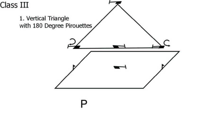
(a)                                             (b)
    Figure 1: (a) Autonomous helicopter. (b) Helicopter hovering under control of learned policy.
Most helicopters are controlled via a 4-dimensional action space:
      • a1 , a2 : The longitudinal (front-back) and latitudinal (left-right) cyclic pitch con-
         trols. The rotor plane is the plane in which the helicopter’s rotors rotate. By
         tilting this plane either forwards/backwards or sideways, these controls cause the
         helicopter to accelerate forward/backwards or sideways.
      • a3 : The (main rotor) collective pitch control. As the helicopter main-rotor’s blades
         sweep through the air, they generate an amount of upward thrust that (generally)
         increases with the angle at which the rotor blades are tilted. By varying the tilt
         angle of the rotor blades, the collective pitch control affects the main rotor’s thrust.
      • a4 : The tail rotor collective pitch control. Using a mechanism similar to the main
         rotor collective pitch control, this controls the tail rotor’s thrust.
Using the position estimates given by the Kalman filter, our task is to pick good control
actions every 50th of a second.
3       Model identification
 To fit a model of the helicopter’s dynamics, we began by asking a human pilot to fly the
 helicopter for several minutes, and recorded the 12-dimensional helicopter state and 4-
 dimensional helicopter control inputs as it was flown. In what follows, we used 339 seconds
 of flight data for model fitting, and another 140 seconds of data for hold-out testing.
 There are many natural symmetries in helicopter flight. For instance, a helicopter at (0,0,0)
 facing east behaves in a way related only by a translation and rotation to one at (10,10,50)
 facing north, if we command each to accelerate forwards. We would like to encode these
 symmetries directly into the model rather than force an algorithm to learn them from
 scratch. Thus, model identification is typically done not in the spatial (world) coordi-
 nates s = [x, y, z, φ, θ, ω, ẋ, ẏ, ż, φ̇, θ̇, ω̇], but instead in the helicopter body coordinates, in
 which the x, y, and z axes are forwards, sideways, and down relative to the current position
 of the helicopter. Where there is risk of confusion, we will use superscript s and b to dis-
 tinguish between spatial and body coordinates; thus, ẋb is forward velocity, regardless of
 orientation. Our model is identified in the body coordinates sb = [φ, θ, ẋb , ẏ b , ż b , φ̇, θ̇, ω̇].
 which has four fewer variables than ss . Note that once this model is built, it is easily
 converted back using simple geometry to one in terms of spatial coordinates.
 Our main tool for model fitting was locally weighted linear regression (e.g., [11, 3]). Given
 a dataset {(xi , yi )}m
                       i=1 where the xi ’s are vector-valued inputs and the yi ’s are the real-
 valued outputs to be predicted, we let X be the design matrix whose i-th row is x i , and let
~y be the vector of yi ’s. In response to a query at x, locally weighted linear regression makes
 the prediction y = β T x, where β = (X T W X)−1 X T W ~y , and W is a diagonal matrix with
 (say) Wii = exp(− 12 (x − xi )T Σ−1 (x − xi )), so that the regression gives datapoints near
 x a larger weight. Here, Σ−1 determines how weights fall off with distance from x, and
 was picked in our experiments via leave-one-out cross validation.1 Using the estimator for
 noise σ 2 given in [3], this gives a model y = β T x + η, where η ∼ Normal(0, σ 2 ). By
    1
        Actually, since we were fitting a model to a time-series, samples tend to be correlated in time,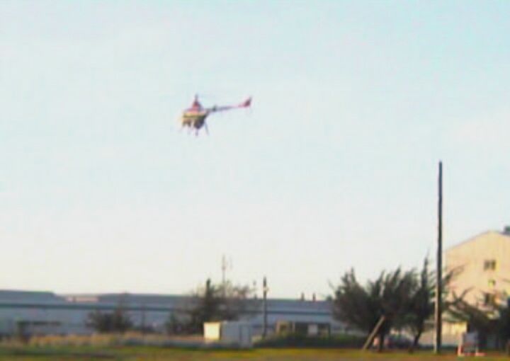
xdot                                                          xdot
                      1                                                            0.5
                                                                                                                2

mean squared error

                                                              mean squared error
                     0.8                                                           0.4

                     0.6                                                           0.3
                                                                                                                1                                 +1
                     0.4                                                           0.2                                                                        Σ   Σ   a1
                                                                                                                                                 errx
                     0.2                                                           0.1                                                             x
                      0                                                             0
                                                                                                                0                                  θ

                                                                                                        ydot
                       0     0.5     1                                               0     0.5      1
                           seconds                                                       seconds
                            xdot                                                         thetadot
                                                                                                                                                 erry
                     0.5                                      0.012                                            −1
                                                                                                                                                   y          Σ   Σ   a2
mean squared error                                                      0.01

                                         mean squared error
                     0.4
                                                                                                                                                   φ
                                                              0.008
                     0.3
                                                              0.006                                            −2
                     0.2
                                                              0.004
                                                                                                                                                 errz         Σ   Σ   a3
                     0.1                                                                                                                           z
                                                              0.002
                                                                                                               −3                                  ω
                      0
                       0     0.5     1
                                                                                    0
                                                                                     0     0.5      1
                                                                                                                 0   2   4          6   8   10                Σ   Σ   a4
                                                                                                                             time                errω
                           seconds                                                       seconds

                                         (a)                                                                             (b)                            (c)
Figure 2: (a) Examples of plots comparing a model fit using the parameterization described in the text
(solid lines) to some other models (dash-dot lines). Each point plotted shows the mean-squared error
between the predicted value of a state variable—when a model is used to the simulate the helicopter’s
dynamics for a certain duration indicated on the x-axis—and the true value of that state variable (as
measured on test data) after the same duration. Top left: Comparison of ẋ-error to model not using
a1s , etc. terms. Top right: Comparison of ẋ-error to model omitting intercept (bias) term. Bottom:
Comparison of ẋ and θ̇ to linear deterministic model identified by [12]. (b) The solid line is the true
helicopter ẏ state on 10s of test data. The dash-dot line is the helicopter state predicted by our model,
given the initial state at time 0 and all the intermediate control inputs. The dotted lines show two
standard deviations in the estimated state. Every two seconds, the estimated state is “reset” to the
true state, and the track restarts with zero error. Note that the estimated state is of the full, high-
dimensional state of the helicopter, but only ẏ is shown here. (c) Policy class. The pictures inside
the circles indicate whether a node outputs the sum of their inputs, or the tanh of the sum of their
inputs. Each edge with an arrow in the picture denotes a tunable parameter. The solid lines show
the hovering policy class (Section 5). The dashed lines show the extra weights added for trajectory
following (Section 6).
applying locally-weighted regression with the state st and action at as inputs, and the one-
step differences (e.g., φt+1 − φt ) of each of the state variables in turn as the target output,
this gives us a non-linear, stochastic, model of the dynamics, allowing us to predict s t+1 as
a function of st and at plus noise.
We actually used several refinements to this model. Similar to the use of body coordinates
to exploit symmetries, there is other prior knowledge that can be incorporated. Since both
φt and φ̇t are state variables, and we know that (at 50Hz) φt+1 ≈ φt + φ̇t /50, there
is no need to carry out a regression for φ. Similarly, we know that the roll angle φ of
the helicopter should have no direct effect on forward velocity ẋ. So, when performing
regression to estimate ẋ, the coefficient in β corresponding to φ can be set to 0. This allows
us to reduce the number of parameters that have to be fit. Similar reasoning allows us to
conclude (cf. [12]) that certain other parameters should be 0, 1/50 or g (gravity), and these
were also hard-coded into the model. Finally, we added three extra (unobserved) variables
a1s , b1s , ω̇f b to model latencies in the responses to the controls. (See [8] for details.)
Some of the (other) choices that we considered in selecting a model include whether to use
the a1s , b1s and/or ω̇f b terms; whether to include an intercept term; at what frequency to
identify the model; whether to hardwire certain coefficients as described; and whether to
use weighted or unweighted linear regression. Our main tool for choosing among the mod-
els was plots such as those shown in Figure 2a. (See figure caption.) We were particularly
interested in checking how accurate a model is not just for predicting st+1 from st , at , but
how accurate it is at longer time scales. Each of the panels in Figure 2a shows, for a model,
the mean-squared error (as measured on test data) between the helicopter’s true position
and the estimated position at a certain time in the future (indicated on the x-axis).
The helicopter’s blade-tip moves at an appreciable fraction of the speed of sound. Given the

and the presence of temporally close-by samples—which will be spatially close-by as well—may
make data seem more abundant than in reality (leading to bigger Σ −1 than might be optimal for test
data). Thus, when leaving out a sample in cross validation, we actually left out a large window (16
seconds) of data around that sample, to diminish this bias.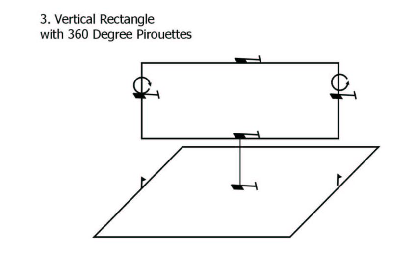
danger and expense (about $70,000) of autonomous helicopters, we wanted to verify the
fitted model carefully, so as to be reasonably confident that a controller tested successfully
in simulation will also be safe in real life. Space precludes a full discussion, but one of
our concerns was the possibility that unmodeled correlations in η might mean the noise
variance of the actual dynamics is much larger than predicted by the model. (See [8] for
details.) To check against this, we examined many plots such as shown in Figure 2b, to
check that the helicopter state “rarely” goes outside the errorbars predicted by our model
at various time scales (see caption).
4     Reinforcement learning: The P EGASUS algorithm
We used the P EGASUS reinforcement learning algorithm of [9], which we briefly review
here. Consider an MDP with state space S, initial state s0 ∈ S, action space A, state
transition probabilities Psa (·), reward function R : S 7→ R, and discount γ. Also let some
family Π of policies π : S 7→ A be given, and suppose our goal is to find a policy in Π with
high utility, where the utility of π is defined to be
                      U (π) = E[R(s0 ) + γR(s1 ) + γ 2 R(s2 ) + · · · |π],
where the expectation is over the random sequence of states s0 , s1 , . . . visited over time
when π is executed in the MDP starting from state s0 .
These utilities are in general intractable to calculate exactly, but suppose we have a com-
puter simulator of the MDP’s dynamics—that is, a program that inputs s, a and outputs
s0 drawn from Psa (·). Then a standard way to define an estimate Û (π) of U (π) is via
Monte Carlo: We can use the simulator to sample a trajectory s0 , s1 , . . ., and by taking the
empirical sum of discounted rewards R(s0 ) + γR(s1 ) + · · · on this sequence, we obtain
one “sample” with which to estimate U (π). More generally, we could generate m such se-
quences, and average to obtain a better estimator. We can then try to optimize the estimated
utilities and search for “arg maxπ Û (π).”
Unfortunately, this is a difficult stochastic optimization problem: Evaluating Û (π) involves
a Monte Carlo sampling process, and two different evaluations of Û (π) will typically give
slightly different answers. Moreover, even if the number of samples m that we average over
is arbitrarily large, Û (π) will fail with probability 1 to be a (“uniformly”) good estimate of
U (π). In our experiments, this fails to learn any reasonable controller for our helicopter.
The P EGASUS method uses the observation that almost all computer simulations of the
form described sample s0 ∼ Psa (·) by first calling a random number generator to get one
(or more) random numbers p, and then calculating s0 as some deterministic function of the
input s, a and the random p. If we demand that the simulator expose its interface to the
random number generator, then by pre-sampling all the random numbers p in advance and
fixing them, we can then use these same, fixed, random numbers to evaluate any policy.
Since all the random numbers are fixed, Û : Π 7→ R is just an ordinary deterministic func-
tion, and standard search heuristics can be used to search for arg maxπ Û (π). Importantly,
this also allows us to show that, so long as we average over a number of samples m that
is at most polynomial in all quantities of interest, then with high probability, Û will be a
uniformly good estimate of U (|Û (π) − U (π)| ≤ ). This also allows us to give guarantees
on the performance of the solutions found. For further discussion of P EGASUS and other
work such as variance reduction and stochastic estimation methods (cf. [5, 10]), see [8].
5   Learning to Hover
One previous attempt had been made to use a learning algorithm to fly this helicopter, using
µ-synthesis [2]. This succeeded in flying the helicopter in simulation, but not on the actual
helicopter (Shim, pers. comm.). Similarly, preliminary experiments using H2 and H∞
controllers to fly a similar helicopter were also unsuccessful. These comments should not
be taken as conclusive of the viability of any of these methods; rather, we take them to be
indicative of the difficulty and subtlety involved in learning a helicopter controller.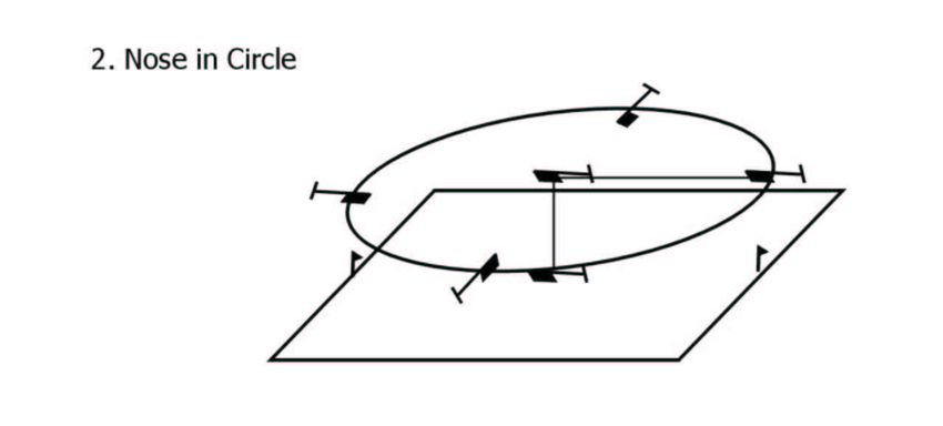
x−velocity (m/s)                                   y−velocity (m/s)                                     z−velocity (m/s)
 1.5                                                0.4                                                     1

   1
                                                    0.2

 0.5                                                                                                   0.5
                                                     0
   0
                                                   −0.2
−0.5                                                                                                        0

                                                   −0.4
 −1

−1.5                                               −0.6                                               −0.5
    0   5   10         15           20   25   30       0   5   10         15           20   25   30       0     5   10         15           20   25   30

                 x−position (m)                                     y−position (m)                                       z−position (m)
 66                                                −45                                                 7

65.5                                               −50
                                                                                                      6.5
 65
                                                   −55
64.5
                                                                                                       6
 64                                                −60

63.5                                               −65                                                5.5
 63
                                                   −70
62.5                                                                                                   5
                                                   −75
 62

61.5                                               −80                                                4.5
    0   5   10         15           20   25   30      0    5   10         15         20     25   30      0      5   10        15          20     25   30

Figure 3: Comparison of hovering performance of learned controller (solid line) vs. Yamaha li-
censed/specially trained human pilot (dotted line). Top: x, y, z velocities. Bottom: x, y, z positions.

We began by learning a policy for hovering in place. We want a controller that, given the
current helicopter state and a desired hovering position and orientation (x∗ , y ∗ , z ∗ , ω ∗ ),
computes controls a ∈ [−1, 1]4 to make it hover stably there. For our policy class Π,
we chose the simple neural network depicted in Figure 2c (solid edges only). Each of
the edges in the figure represents a weight, and the connections were chosen via simple
reasoning about which control channel should be used to control which state variables.
For instance, consider the longitudinal (forward/backward) cyclic pitch control a 1 , which
causes the rotor plane to tilt forward/backward, thus causing the helicopter to pitch (and/or
accelerate) forward or backward. From Figure 2c, we can read off the a1 control as
 t1 = w1 + w2 errxb + w3 tanh(w4 errxb ) + w5 ẋb + w6 θ; a1 = w7 tanh(w8 t1 ) + w9 t1 .
Here, the wi ’s are the tunable parameters (weights) of the network, and errxb = xb −
xbdesired is defined to be the error in the xb -position (forward direction, in body coordinates)
between where the helicopter currently is and where we wish it to hover.
We chose a quadratic cost function on the (spatial representation of the) state, where 2
  R(s) = −(αx (x−x∗ )2 +αy (y −y ∗ )2 +αz (z −z ∗ )2 +αẋ ẋ2 +αẏ ẏ 2 +αż ż 2 +αω (ω −ω ∗ )2 ). (1)
This encourages the helicopter to hover near (x∗ , y ∗ , z ∗ , ω ∗ ), while also keeping the veloc-
ity small and not making abrupt movements. The weights αx , αy , etc. (distinct from the
weights wi parameterizing our policy class) were chosen to scale each of the terms to be
roughly the same order of magnitude. To encourage small actions and smooth control of
the helicopter, we also used a quadratic penalty for actions: R(a) = −(αa1 a21 + αa2 a22 +
αa3 a23 + αa4 a24 ), and the overall reward was R(s, a) = R(s) + R(a).
Using the model identified in Section 3, we can now apply P EGASUS to define approx-
imations Û (π) to the utilities of policies. Since policies are smoothly parameterized in
the weights, and the dynamics are themselves continuous in the actions, the estimates of
utilities are also continuous in the weights.3 We may thus apply standard hillclimbing al-
gorithms to maximize Û (π) in terms of the policy’s weights. We tried both a gradient
    2
      The ω −ω ∗ error term is computed with appropriate wrapping about 2π rad, so that if ω ∗ = 0.01
rad, and the helicopter is currently facing ω = 2π − 0.01 rad, the error is 0.02, not 2π − 0.02 rad.
    3
      Actually, this is not true. One last component of the reward that we did not mention earlier was
that, if in performing the locally weighted regression, the matrix X T W X is singular to numerical
precision, then we declare the helicopter to have “crashed,” terminate the simulation, and give it
a huge negative (-50000) reward. Because the test checking if X T W X is singular to numerical
precision returns either 1 or 0, Û (π) has a discontinuity between “crash” and “not-crash.”
10
9.5
9.5
9
9
8.5
8.5
8 −58
6.4 8 −71
7.5 −59 6.2
6
7.5 −72
−60
7 82 −73
−61 7
80 −74
6.5 −62 78 6.5 −75
−63 −90
6 76 −76
−64 74 6
−95 −77
5.5 −65 72 5.5 −78
70 −100
−66 −79
68
−67 68.5 −80
64 66 −105 68
63.5 −68 64 67.5 −81
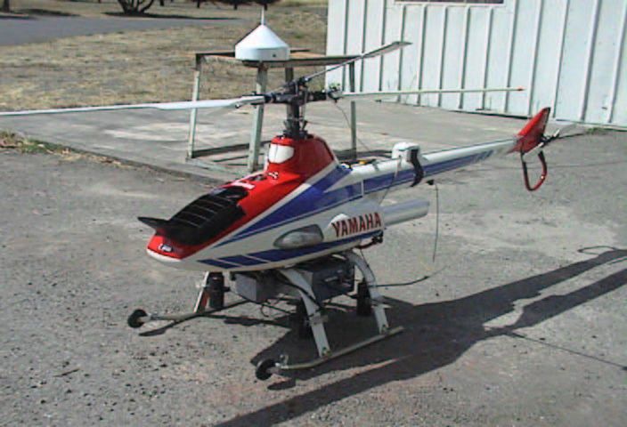
Figure 4: Top row: Maneuver diagrams from RC helicopter competition. [Images courtesy of the
Academy of Model Aeronautics.] Bottom row: Actual trajectories flown using learned controller.
ascent algorithm, in which we numerically evaluate the derivative of Û (π) with respect to
the weights and then take a step in the indicated direction, and a random-walk algorithm
in which we propose a random perturbation to the weights, and move there if it increases
Û (π). Both of these algorithms worked well, though with gradient ascent, it was important
to scale the derivatives appropriately, since the estimates of the derivatives were sometimes
numerically unstable.4 It was also important to apply some standard heuristics to prevent
its solutions from diverging (such as verifying after each step that we did indeed take a step
uphill on the objective Û , and undoing/redoing the step using a smaller stepsize if this was
not the case).
The most expensive step in policy search was the repeated Monte Carlo evaluation to obtain
Û (π). To speed this up, we parallelized our implementation, and Monte Carlo evaluations
using different samples were run on different computers, and the results were then aggre-
gated to obtain Û (π). We ran P EGASUS using 30 Monte Carlo evaluations of 35 seconds
of flying time each, and γ = 0.9995. Figure 1b shows the result of implementing and
running the resulting policy on the helicopter. On its maiden flight, our learned policy was
successful in keeping the helicopter stabilized in the air. (We note that [1] was also suc-
cessful at using our P EGASUS algorithm to control a subset, the cyclic pitch controls, of a
helicopter’s dynamics.)
We also compare the performance of our learned policy against that of our human pilot
trained and licensed by Yamaha to fly the R-50 helicopter. Figure 3 shows the velocities and
positions of the helicopter under our learned policy and under the human pilot’s control. As
we see, our controller was able to keep the helicopter flying more stably than was a human
pilot. Videos of the helicopter flying are available at
http://www.cs.stanford.edu/˜ang/rl/
6 Flying competition maneuvers
We were next interested in making the helicopter learn to fly several challenging maneu-
vers. The Academy of Model Aeronautics (AMA) (to our knowledge the largest RC heli-
copter organization) holds an annual RC helicopter competition, in which helicopters have
to be accurately flown through a number of maneuvers. This competition is organized into
Class I (for beginners, with the easiest maneuvers) through Class III (with the most difficult
maneuvers, for the most advanced pilots). We took the first three maneuvers from the most
challenging, Class III, segment of their competition.
Figure 4 shows maneuver diagrams from the AMA web site. In the first of these maneuvers
4
A problem exacerbated by the discontinuities described in the previous footnote.(III.1), the helicopter starts from the middle of the base of a triangle, flies backwards to the lower-right corner, performs a 180◦ pirouette (turning in place), flies backwards up an edge of the triangle, backwards down the other edge, performs another 180◦ pirouette, and flies backwards to its starting position. Flying backwards is a significantly less stable maneuver than flying forwards, which makes this maneuver interesting and challenging. In the second maneuver (III.2), the helicopter has to perform a nose-in turn, in which it flies backwards out to the edge of a circle, pauses, and then flies in a circle but always keeping the nose of the helicopter pointed at center of rotation. After it finishes circling, it returns to the starting point. Many human pilots seem to find this second maneuver particularly challenging. Lastly, maneuver III.3 involves flying the helicopter in a vertical rectangle, with two 360 ◦ pirouettes in opposite directions halfway along the rectangle’s vertical segments. How does one design a controller for flying trajectories? Given a controller for keeping a system’s state at a point (x∗ , y ∗ , z ∗ , ω ∗ ), one standard way to make the system move through a particular trajectory is to slowly vary (x∗ , y ∗ , z ∗ , ω ∗ ) along a sequence of set points on that trajectory. (E.g., see [4].) For instance, if we ask our helicopter to hover at (0, 0, 0, 0), then a fraction of a second later ask it to hover at (0.01, 0, 0, 0), then at (0.02, 0, 0, 0) and so on, our helicopter will slowly fly in the xs -direction. By taking this procedure and “wrapping” it around our old policy class from Figure 2c, we thus obtain a computer program—that is, a new policy class—not just for hovering, but also for flying arbitrary trajectories. I.e., we now have a family of policies that take as input a trajectory, and that attempt to make the helicopter fly that trajectory. Moreover, we can now also retrain the policy’s parameters for accurate trajectory following, not just hovering. For flying trajectories, we also augmented the policy class to take into account more of the coupling between the helicopter’s different subdynamics. For instance, the simplest way to turn is to change the tail rotor collective pitch/thrust, so that it yaws either left or right. This works well for small turns, but for large turns, the thrust from the tail rotor also tends to cause the helicopter to drift sideways. Thus, we enriched the policy class to allow it to correct for this drift by applying the appropriate cyclic pitch controls. Also, having a helicopter climb or descend changes the amount of work done by the main rotor, and hence the amount of torque/anti-torque generated, which can cause the helicopter to turn. So, we also added a link between the collective pitch control and the tail rotor control. These modifications are shown in Figure 2c (dashed lines). We also needed to specify a reward function for trajectory following. One simple choice for R would have been to use Equation (1) with the newly-defined (time-varying) (x∗ , y ∗ , z ∗ , ω ∗ ). But we did not consider this to be a good choice. Specifically, consider making the helicopter fly in the increasing x-direction, so that (x∗ , y ∗ , z ∗ , ω ∗ ) starts off as (0, 0, 0, 0) (say), and has its first coordinate x∗ slowly increased over time. Then, while the actual helicopter position xs will indeed increase, it will also almost certainly lag con- sistently behind x∗ . This is because the hovering controller is always trying to “catch up” to the moving (x∗ , y ∗ , z ∗ , ω ∗ ). Thus, x − x∗ may remain large, and the helicopter will continuously incur a x − x∗ cost, even if it is in fact flying a very accurate trajectory in the increasing x-direction exactly as desired. It would be undesirable to have the helicopter risk trying to fly more aggressively to reduce this fake “error,” particularly if it is at the cost of increased error in the other coordinates. So, we changed the reward function to penal- ize deviation not from (x∗ , y ∗ , z ∗ , ω ∗ ), but instead deviation from (xp , yp , zp , ωp ), where (xp , yp , zp , ωp ) is the “projection” of the helicopter’s position onto the path of the idealized, desired trajectory. (In our example of flying in a straight line, for a helicopter at (x, y, z, ω), we easily see (xp , yp , zp , ωp ) = (x, 0, 0, 0).) Thus, we imagine an “external observer” that looks at the actual helicopter state and estimates which part of the idealized trajectory the helicopter is trying to fly through (taking care not to be confused if a trajectory loops back on itself), and the learning algorithm pays a penalty that is quadratic between the actual position and the “tracked” position on the idealized trajectory. We also needed to make sure the helicopter is rewarded for making progress along the
trajectory. To do this, we used the potential-based shaping rewards of [7]. Since, we are
already tracking where along the desired trajectory the helicopter is, we chose a potential
function that increases along the trajectory. Thus, whenever the helicopter’s (x p , yp , zp , ωp )
makes forward progress along this trajectory, it receives positive reward. (See [7].)
Finally, our modifications have decoupled our definition of the reward function from
(x∗ , y ∗ , z ∗ , ω ∗ ) and the evolution of (x∗ , y ∗ , z ∗ , ω ∗ ) in time. So, we are now also free
to consider allowing (x∗ , y ∗ , z ∗ , ω ∗ ) to evolve in a way that is different from the path of the
desired trajectory, but nonetheless in a way that allows the helicopter to follow the actual,
desired trajectory more accurately. (In control theory, there is a related practice of using the
inverse dynamics to obtain better tracking behavior.) We considered several alternatives,
but the main one used ended up being a modification for flying trajectories that have both
a vertical and a horizontal component (such as along the two upper edges of the triangle in
III.1). Specifically, it turns out that the z (vertical)-response of the helicopter is very fast:
To climb, we need only increase the collective pitch control, which almost immediately
causes the helicopter to start accelerating upwards. In contrast, the x and y responses are
much slower. Thus, if (x∗ , y ∗ , z ∗ , ω ∗ ) moves at 45◦ upwards as in maneuver III.1, the he-
licopter will tend to track the z-component of the trajectory much more quickly, so that it
accelerates into a climb steeper than 45◦ , resulting in a “bowed-out” trajectory. Similarly,
an angled descent results in a “bowed-in” trajectory. To correct for this, we artificially
slowed down the z-response, so that when (x∗ , y ∗ , z ∗ , ω ∗ ) is moving into an angled climb
or descent, the (x∗ , y ∗ , ω ∗ ) portion will evolve normally with time, but the changes to z ∗
will be delayed by t seconds, where t here is another parameter in our policy class, to be
automatically learned by our algorithm.
Using this setup and retraining our policy’s parameters for accurate trajectory following,
we were able to learn a policy that flies all three of the competition maneuvers fairly ac-
curately. Figure 4 (bottom) shows actual trajectories taken by the helicopter while flying
these maneuvers. Videos of the helicopter flying these maneuvers are also available at the
URL given at the end of Section 5.

References
 [1] J. Bagnell and J. Schneider. Autonomous helicopter control using reinforcement
     learning policy search methods. In Int’l Conf. Robotics and Automation. IEEE, 2001.
 [2] G. Balas, J. Doyle, K. Glover, A. Packard, and R. Smith. µ-analysis and synthesis
     toolbox user’s guide, 1995.
 [3] W. Cleveland. Robust locally weighted regression and smoothing scatterplots. J.
     Amer. Stat. Assoc, 74, 1979.
 [4] Gene F. Franklin, J. David Powell, and Abbas Emani-Naeini. Feedback Control of
     Dynamic Systems. Addison-Wesley, 1995.
 [5] J. Kiefer and J. Wolfowitz. Stochastic estimation of the maximum of a regression
     function. Annals of Mathematical Statistics, 23:462–466, 1952.
 [6] J. Leishman. Principles of Helicopter Aerodynamics. Cambridge Univ. Press, 2000.
 [7] A. Y. Ng, D. Harada, and S. Russell. Policy invariance under reward transformations:
     Theory and application to reward shaping. In Proc. 16th ICML, pages 278–287, 1999.
 [8] Andrew Y. Ng. Shaping and policy search in reinforcement learning. PhD thesis,
     EECS, University of California, Berkeley, 2003.
 [9] Andrew Y. Ng and Michael I. Jordan. P EGASUS: A policy search method for large
     MDPs and POMDPs. In Proc. 16th Conf. Uncertainty in Artificial Intelligence, 2000.
[10] Herbert Robbins and Sutton Monro. A stochastic approximation method. Annals of
     Mathematical Statistics, 22:40–407, 1951.
[11] C. Atkeson S. Schaal and A. Moore. Locally weighted learning. AI Review, 11, 1997.
[12] Hyunchul Shim. Hierarchical flight control system synthesis for rotorcraft-based un-
     manned aerial vehicles. PhD thesis, Mech. Engr., U.C. Berkeley, 2000.
You can also read