Recovering Intrinsic Images with a Global Sparsity Prior on Reflectance
←
→
Page content transcription
If your browser does not render page correctly, please read the page content below
Recovering Intrinsic Images with a Global Sparsity
                   Prior on Reflectance

               Peter Vincent Gehler                                 Carsten Rother
          Max Planck Institut for Informatics                 Microsoft Research Cambridge
                  pgehler@mpii.de                              carrot@microsoft.com

                        Martin Kiefel, Lumin Zhang, Bernhard Schölkopf
                           Max Planck Institute for Intelligent Systems
                           {mkiefel,lumin,bs}@tuebingen.mpg.de

                                              Abstract
         We address the challenging task of decoupling material properties from lighting
         properties given a single image. In the last two decades virtually all works have
         concentrated on exploiting edge information to address this problem. We take a
         different route by introducing a new prior on reflectance, that models reflectance
         values as being drawn from a sparse set of basis colors. This results in a Random
         Field model with global, latent variables (basis colors) and pixel-accurate output
         reflectance values. We show that without edge information high-quality results
         can be achieved, that are on par with methods exploiting this source of informa-
         tion. Finally, we are able to improve on state-of-the-art results by integrating edge
         information into our model. We believe that our new approach is an excellent
         starting point for future developments in this field.

1    Introduction
The task of recovering intrinsic images is to separate a given input image into its material-dependent
properties, known as reflectance or albedo, and its light-dependent properties, such as shading, shad-
ows, specular highlights, and inter-reflectance. A successful separation of these properties would be
beneficial to a number of computer vision tasks. For example, an image which solely depends on
material-dependent properties is helpful for image segmentation and object recognition [11], while
a clean image of shading is a valuable input to shape-from-shading algorithms.
As in most previous work in this field, we cast the intrinsic image recovery problem into the follow-
ing simplified form, where each image pixel is the product of two components:
                                               I = sR .                                              (1)
            3                                             3
Here I ∈ R is the pixel’s color, in RGB space, R ∈ R is its reflectance and s ∈ R its “shading”.
Note, we use “shading” as a proxy for all light-dependent properties, e.g. shadows. The fact that
shading is only a 1D entity imposes some limitations. For example, shading effects stemming from
multiple light sources can only be modeled if all light sources have the same color.1 The goal of this
work is to estimate s and R given I. This problem is severely under-constraint, with 4 unknowns
and 3 constraints for each pixel. Hence, a trivial solution to (1) is, for instance, I = R, s = 1 for all
pixels. The main focus of this paper is on exploring sensible priors for both shading and reflectance.
Despite the importance of this problem surprisingly little research has been conducted in recent
years. Most of the inventions were done in the 70s and 80s. The recent comparative study [7] has
shown that the simple Retinex method [9] from the 70s is still the top performing approach. Given
   1
     This problem can be overcome by utilizing a 3D vector for s, as done in [4], which we however do not
consider in this work.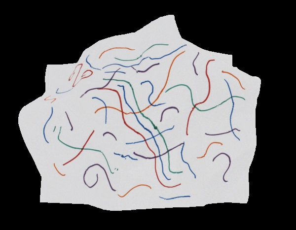
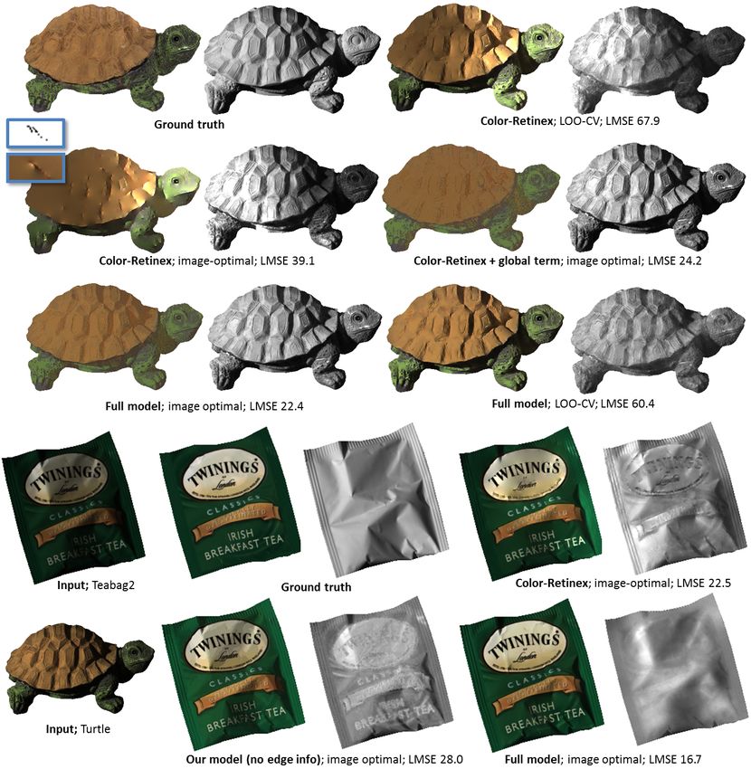
(a) Image I “paper1”         (b) I (in RGB)        (c) Reflectance R       (d) R (in RGB)          (e) Shading s

Figure 1: An image (a), its color in RGB space (b), the reflectance image (c), its distribution in
RGB space (d), and the shading image (e). Omer and Werman [12] have shown that an image of
a natural scene often contains only a few different “basis colorlines”. Figure (b) shows a dominant
gray-scale color-line and other color lines corresponding to the scribbles on the paper (a). These
colorlines are generated by taking a small set of “basis colors” which are then linearly “smeared”
out in RGB space. The basis colors are clearly visible in (d), where the cluster for white (top,
right) is the dominant one. This “smearing effect” comes from properties of the scene (e.g. shading
or shadows), and/or properties of the camera, e.g. motion blur. (Note, the few pixels in-between
clusters are due to anti-aliasing effects). In this work we approximate the basis colors by a simple
mixture of isotropic Gaussians.

the progress in the last two decades on probabilistic models, inference and learning techniques, as
well as the improved computational power, we believe that now is a good time to revisit this problem.
This work, together with the recent papers [14, 4, 7, 15], are a first step in this direction.
The main motivation of our work is to develop a simple, yet powerful probabilistic model for shading
and reflectance estimation. In total we use three different types of factors. The first one is the
most commonly used factor and is key ingredient of all Retinex-based methods. The idea is to
extract those image edges which are (potentially) true reflectance edges and then to recover a new
reflectance image that contains only these edges, using a set of Poisson equations. This term on
its own is enough to recover a non-trivial decomposition, i.e. s 6= 1. The next factor is a simple
smoothness prior on shading between neighboring image pixels, and has been used by some previous
work e.g. [14]. Note, there are a few works, which we discuss in more detail later, that extend these
pairwise terms to become patch-based. The third prior term is the main contribution of our work and
is conceptually very different from the local (pairwise or patch-based) constraints of previous works.
We propose a new global (image-wide) sparsity prior on reflectance based on the findings of [12]
and discussed in Fig 1. In the absence of other factors this already produces non-trivial results. This
prior takes the form of a Mixture of Gaussians, and encodes the assumption that the reflectance value
for each pixel is drawn from some mixing components, which in this context we refer to as “basis
colors”. The complete model forms a latent variable Random Field model for which we perform
MAP estimation.
By combining the different terms we are able to outperform state-of-the art. If we use image optimal
parameter settings we perform on par with methods that use multiple images as input. To empirically
validate this we use the database introduced in the comparative study [7].

2        Related Work
There is a vast amount of literature on the problem of recovering intrinsic images. We refer the
reader to detailed surveys in [8, 17, 7], and limit our attention to some few related works.
Barrow and Tenenbaum [2] were the first to define the term “intrinsic image”. Around the same
time the first solution to this problem was developed by Land and McCann [9] known as the Retinex
algorithm. After that the Retinex algorithm was extended to two dimensions by Blake [3] and
Horn [8], and later applied to color images [6]. The basic Retinex algorithm is a 2-step procedure:
1) detect all image gradients which are caused by changes in reflectance; 2) recover a reflectance
image which preserves the detected reflectance gradients. The basic assumption of this approach
is that small image gradients are more likely caused by a shading effect and strong gradients by a
change in reflectance. For color images this rule can be extended by treating changes in the 1D
brightness domain differently to changes in the 2D chromaticity space.2 This method, which we
denote as “Color Retinex” was the top performing method in the recent comparison paper [7]. Note,
     2
         Note, a gradient in chromaticity can only be caused by differently colored light sources, or inter-reflectance.

                                                             2
the only approach which could beat Retinex utilizes multiple images [19]. Surprisingly, the study
[7] also shows that more sophisticated methods for training the reflectance edge detector, using
e.g. images patches, did not perform better than the basic Retinex method. In particular the study
tested two methods of Tappen et al. [17, 16]. A plausible explanation is offered, namely that these
methods may have over-fitted the small amount of training data. The method [17] has an additional
intermediate step where a Markov Random Field (MRF) is used to “propagate” reflectance gradients
along contour lines.
The paper [15] implements the same intuition as done here, namely that there is a sparse set of re-
flectances present in the scene. However both approaches bear the following differences. In [15] a
sparsity enforcing term is included, that is penalizing reflectance differences from some prototype
references. This term encourages all reflectances to take on the same value, while the model we
propose in this paper allows for a mixture of different material reflectances and thus keeps their
diversity. Also, in contrast to [15], where a gradient aware wavelet transform is used as a new
representation, here we work directly in the RGB domain. By doing so we directly extend previ-
ous intrinsic image models which makes evident the gains that can be attributed to a global sparse
reflectance term alone.
Recently, Shen et al. [14] introduced an interesting extension of the Retinex method, which bears
some similarity with our approach. The key idea in their work is to perform a pre-processing step
where the (normalized) reflectance image is partitioned into a few clusters. Each cluster is treated
as a non-local “super-pixel”. Then a variant of the Retinex method is run on this super-pixel image.
The conceptual similarity to our approach is the idea of performing an image-wide clustering step.
However, the differences are that they do not formulate this idea as a joint probabilistic model over
latent reflectance “basis colors” and shading variables. Furthermore, every pixel in a super-pixel
must have the same intensity, which is not the case in our work. Also, they need a Retinex type of
edge term to avoid the trivial solution of s = 1.
Finally, let us briefly mention techniques which use patch-based constraints, instead of pair-wise
terms. The seminal work of Freeman et al. on learning low-level vision [5] formulates a probabilistic
model for intrinsic images. In essence, they build a patch-based prior jointly over shading and
reflectance. In a new test image the best explanation for reflectance and shading is determined.
The key idea is that patches do overlap, and hence form an MRF, where long-range propagation
is possible. Since no large-scale ground database was available at that time, they only train and
test on computer generated images of blob-like textures. Another patch-based method was recently
suggested in [4]. They introduce a new energy term which is satisfied when all reflectance values
in a small, e.g. 3 × 3, patch lie on a plane in RGB space. This idea is derived from the Laplacian
matrix used for image matting [10]. On its own this term gives in practice often the trivial solution
s = 1. For that reason additional user scribbles are provided to achieve high-quality results.3

3       A Probabilistic Model for Intrinsic Images
The model outlined here falls into the class of Conditional Random Fields, specifying a conditional
probability distribution over reflectance R and shading S components for a given image I
                                       p(s, R | I) ∝ exp (−E(s, R | I)) .                                     (2)
Before we describe the energy function E in detail, let us specify the notation. We will denote with
subscripts i the values at location i in the image. Thus Ii is an image pixel (vector of dimension 3),
Ri a reflectance vector (a 3-vector), si the shading (a scalar). The total number of pixels in an image
is N . With boldface we denote vectors of components, e.g. s = (s1 , . . . , sN ).
There are two ways to use the relationship (1) to formulate a model for shading and reflectance,
corresponding to two different image likelihoods p(I | s, R). One possible way is to relax the
relation (1) and for example assume a Gaussian likelihood p(I | s, R) ∝ exp(−kI − sRk2 ) to
account for some noise in the image formation process. This yields an optimization problem with
4N unknowns. The second possibility is to assume a delta-prior around sR which results in the
following complexity reduction. Since Iic = si Ric has to hold of all color channels c = {R, G, B},
the unknown variables are specified up to scalar multipliers, in other words the direction of Ri is
already known. We rewrite Ri = ri R  ~ i , with R
                                                ~ i = Ii /kIi k, leaving r = (r1 , . . . , rN ) to be the
    3
        We performed initial tests with this term. However, we found that it did not help to improve performance.

                                                         3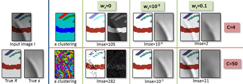
only unknown variable. The shading components can be computed using si = kIi k/ri . Thus the
optimization problem is reduced to a search of N variables.
The latter reduction is commonly exploited by intrinsic image algorithms in order to simplify the
model [7, 14, 4] and in the remainder we will also make use of it. This allows us to write all model
parts in terms of r.
Note that there is a global scalar k by which the result s, R can be modified without effecting eq. (1),
i.e. I = (sk)(1/kR). For visualization purpose k is chosen such that the results are visually closest
to the known ground truth.

3.1   Model
The energy function we describe here consists of three different terms that are linearly combined.
We will describe the three components and their influence in greater detail below, first we write the
optimization problem that corresponds to a MAP solution in its most general form
                            min    ws Es (r) + wr Eret (r) + wcl Ecl (r, α).                      (3)
                         ri ,αi ;i=1,...,n

Note, the global scale of the energy is not important, hence we can always fix one non-zero weight
ws , wr , wcl to 1.

Shading Prior (Es ) We expect the shading of an image to vary smoothly over the image and we
encode this in the following pairwise factors
                                         X                           2
                               Es (r) =       ri−1 kIi k − rj−1 kIj k ,                   (4)
                                             i∼j

where we use a 4-connected pixel graph to encode the neighborhood relation which we denote with
i ∼ j. Because of the dependency on the inverse of r, this term is not jointly convex in r. Any
model that includes this smoothness prior thus has the (potential) problem of multiple local minima.
Empirically we have seen that, however, this function seems to be very well behaved, a large range of
different starting points for r resulted in the same minimum. Nevertheless, we use multiple restarts
with different starting points, see optimization selection 3.2.

Gradient Consistency (Eret ) As discussed in the introduction, the main idea of the Retinex algo-
rithm is to disambiguate between edges that are due to shading variations from those that are caused
by material reflectance changes. This idea is then implemented as follows. Assume that we already
know, or have classified, that an edge at location i, j in the input image is caused by a change in re-
flectance. Then we know the magnitude of the gradient that has to appear in the reflectance map by
noting that log(Ii )−log(Ij ) = log(ri R~ i )−log(rj R
                                                     ~ j ). Using the fact log(kIi k) = log(I c )−log(R
                                                                                                      ~ c)
                                                                                             i          i
(for all channels c) and assuming a squared deviation around the log gradient magnitude, this trans-
lates into the following Gaussian MRF term on the reflectances
                           X                                                             2
                Eret (r) =     (log(ri ) − log(rj ) − gij (I)(log(kIi k) − log(kIj k))) .              (5)
                           i∼j
It remains to specify the classification function g(I) for the image edges. In this work we adopt the
Color Retinex version that has been proposed in [7]. For each pixel i and a neighbor j we compute
the gradient of the intensity image and the gradient of the chromaticity change. If both gradients
exceed a certain threshold (θg and θc resp.), the edge at i, j is classified as being a “reflectance edge”
and in this case gij (I) = 1. The two parameters which are the thresholds θg , θc for the intensity
and the chromaticity change are then estimated using leave-one-out-cross validation. It is worth
noting that this term is qualitatively different from the smoothness prior on shading (4) even for
pixels where gij (I) = 0. Here, the log-difference is penalized whereas the shading smoothness
does also depend on the intensity values kIi k, kIj k. By setting wcl , ws = 0 in Eq. (2) we recover
Color Retinex [7].
Global Sparse Reflectance Prior (Ecl ) Motivated by the findings of [12] we include a term
that acts as a global potential on the reflectances and favors the decomposition into some few
reflectance clusters. We assume C different reflectance clusters, each of which is denoted by
R̃c , c ∈ {1, . . . , C}. Every reflectance component ri belongs to one of the clusters and we de-
note its cluster membership with the variable αi ∈ {1, . . . , C}. This is summarized in the following
energy term

                                                    4
Figure 2: A crop from the image “panther”. Left: input image I and true decomposition (R, s). Note,
the colors in reflectance image (True R) have been modified on purpose such that there are exactly 4
different colors. The second column shows a clustering (here from the solution with ws = 0), where
each cluster has an arbitrary color. The remaining columns show results with various settings for C
and ws (left reflectance image, right shading image). Top row is the result for C = 4 and bottom
row for C = 50 clusters, columns are results for ws = 0, 10−5 , and 0.1. Below the images is the
corresponding LMSE score (described in Section 4.1). (Note, results are visually slightly different
since the unknown overall global scaling factor k is set differently, that is I = (sk)(1/kR).
n
X
Ecl (r, α) = ~ i − R̃α k2 .
kri R (6)
i
i=1
Here, both continuous r and discrete α variables are mixed. This represents a global potential, since
the cluster means depend on the assignment of all pixels in the image. For fixed α, this term is
convex in r and for fixed r the optimum of α is a simple assignment problem. The cluster means R̃c
~ i.
are optimally determined given r and α: R̃c = |{i:α1i =c}| i:αi =c ri R
P
Relationship between Ecl and Es The example in Figure 2 highlights the influence of the terms.
We use a simplified model (2), namely Ecl + ws Es , and vary ws as well as the number of clusters.
Let us first consider the case where ws = 0 (third column). Independent of the clustering we
get an imperfect result. This is expected since there is no constraint across clusters. Hence the
shading within one cluster looks reasonable, but is not aligned across clusters. By adding a little
bit of smoothing (ws = 10−5 ; 4’th column), this problem is cured for both clusterings. It is very
important to note that too many clusters (here C=50) do not affect the result very much. The reason
is that enough clustering constraints are present to recover the variation in shading. If we were to
give each pixel its own cluster this would no longer be true and we would get the trivial solution of
s = 1. Finally, results deteriorate when the smoothing term is too strong (last column ws = 0.1),
since it prefers a constant shading. Note, that for this simple toy example the smoothness prior was
not important, however for real images the best results are achieved by using a non-zero ws .
3.2 Optimization of (3)
Algorithm 1 Coordinate Descent for solving (3)
The MAP problem (3) consists of 1: Select r 0 as described in the text
both discrete and continuous vari- 2: α0 ← K-Means clustering of {ri0 R ~ i , i = 1, . . . , N }
ables and we solve it using coordinate 3: t ← 0
descent. The entire algorithm is sum- 4: repeat
marized in Algorithm 1. 4 5: rt+1 ← optimize (3) with αt fixed
Given an initial value for α we have 6:
P
R̃c = i:αi =c ri R ~ i /|{i : αi = c}|
t+1
seen empirically that our function 7: α ← assign new cluster labels with rt+1 fixed
tends to yield same solutions, irre- 8: t←t+1
spective of the starting point r. In or- 9: until E(rt−1 , αt−1 ) − E(rt , αt ) < θ
der to be also robust with respect to
this initial choice, we choose from a range of initial r values as described next. From these start-
ing points we choose the one with the lowest objective value (energy) and its corresponding result.
4
Code available http://people.tuebingen.mpg.de/mkiefel/projects/intrinsic
5comment Es Ecl Eret LOO-CV best single image opt.
Color Retinex - - X 29.5 29.5 25.5
no edge information X X - 30.0 30.6 18.2
Col-Ret+ global term - X X 27.2 24.4 18.1
full model X X X 27.4 24.4 16.1
Table 1: Comparing the effect of including different terms. The column “best-single” is the pa-
rameter set that works best on all 16 images jointly, “image opt.” is the result when choosing the
parameters optimal for each image individually, based on ground truth information.
We have seen empirically that this procedure gives stable results. For instance, we virtually always
achieve a lower energy compared to using the ground truth r as initial start point.
Initialization of r It is reasonable to assume that the output has a fixed range, i.e. 0 ≥ Ric , si ≥ 1
(for all c, i).5 In particular, this is true for the data in [7]. From these constraints we can derive
that kIi k ≥ ri ≥ 3. Given that, we use the following three starting points for r, by varying γ ∈
{0.3, 0.5, 0.7}: ri = γkIi k + 3(1 − γ). Additionally we choose the start point r = 1. From these
four different initial settings we choose the result which corresponds to the lowest final energy.
Initialization of α Given an initial value for r we can compute the terms in Eq.(6) and use K-
Means clustering to optimize it. We use the best solution from five restarts.
Updating r for a given fixed α this is implemented using a conjugate gradient descent solver [1].
This typically converges in some few hundred iterations for the images used in the experiments.
Updating α ~ i − R̃c k2 .
for given r this is a simple assignment problem: αi = argminc=1,...,C kri R
4 Experiments
For the empirical evaluation we use the intrinsic image database that has been introduced in [7].
This dataset consists of 16 different images for all of which the ground truth shading and reflectance
components are available. We refer to [7] for details on how this data was collected. Some of the
images can be seen in Figure 3. In all experiments we compare against Color Retinex which was
found to be the best performing method among those that take a single image as input. The method
from [19] yields better results but requires multiple input images from different light variations.
4.1 Error metric
We report the performance of the algorithms using the two different error metrics that have been
suggested by the creators of the database [7]. The first metric is the average of the localized mean
squared error (LMSE) between the predicted and true shading and predicted and true reflectance
image. 6 Since the LMSE vary considerably we also use the average rank of the algorithm.
4.2 Experimental set-up and parameter learning
All free parameters of the models, e.g. the weights wcl , ws , wr and the gradient thresholds θc , θg
have been chosen using a leave-one-out estimate (LOO-CV). Due to the high variance of the scores
for the images we used the median error to score the parameters. Thus for image i the parameter
was chosen that leads to the lowest median error on all images except i. Additionally we record the
best single parameter set that works well on all images, and the score that is obtained when using
the optimal parameters on each image individually. Although the latter estimate involves knowing
ground truth estimates we are interested in the lower bound of the performance, in an interactive
scenario a user can provide additional information to achieve this, as in [4].
We select the parameters from the following ranges. Whenever used, we fix wcl = 1 since it
suffices to specify the relative difference between the parameters. For models using both the cluster
and shading smoothness terms, we select from ws ∈ {0.001, 0.01, 0.1}, for models that use the
cluster and Color Retinex term wr ∈ {0.001, 0.01, 0.1, 1, 10}. When all three terms are non-zero,
we vary ws as above paired with wr ∈ ×{0.1ws , ws , 10ws }. The gradient thresholds are varied
in θg , θc ∈ {0.075, 1} which yields four possible configurations. The reflectance cluster count is
varied in C ∈ {10, 50, 150}.
5
This assumption is violated if there is no global scalar k such that 0 ≥ (1/kRic ), (ksi ) ≥ 1.
6
We multiply by 1000 for easier readability
64.3 Comparison - Model variations
In a first set of experiments we investigate the influence of using combinations of the prior terms
described in Section 3.1. The numerical results are summarized in Table 1.
The first observation is that the Color Retinex algorithm (1st row) performs about similar to the
system using a shading smoothness prior together with the global factor Ecl (2nd row). Note that
the latter system does not use any gradient information for estimation. This confirms our intuition
that the term Ecl provides strong coupling information between reflectance components, as also
discussed in Figure 2. The lower value for the image optimal setting of 18.2 compared to 25.5 for
Color Retinex indicates that one would benefit from a better parameter estimate, i.e. the flexibility
of this algorithm is higher. Equipping Color Retinex with the global reflectance term improves all
recorded results (3rd vs 2nd row). Again it seems that the LOO-CV parameter estimation is more
stable in this case. Combining all three parts (4th row) does not improve the results over Color
Retinex with the reflectance prior. With knowledge about the optimal image parameter it yields a
lower LMSE score (16.1 vs 18.1).
LOO-CV rank best single im. opt.
4.4 Comparison to Literature TAP05 [17] 56∗ - - -
TAP06 [16] 39∗ - - -
In Table 2 we compare the numer- SHE [14]+ n/a n/a 56.2 n/a
ical results of our method to other
SHE [15]× n/a n/a (20.4) -
intrinsic image algorithms. We
BAS [7] 72.6 5.1 60.3 36.6
again include the single best pa-
Gray-Ret [7] 40.7 4.9 40.7 28.9
rameter and image dependent opti-
Col-Ret 29.5 3.7 29.5 25.5
mal parameter set. Although those
full model 27.4 3.0 24.4 16.1
are positively biased and obviously
decrease with model complexity Weiss [19] 21.5 2.7 21.5 21.5
we believe that they are informa- Weiss+Ret [7] 16.4 1.7 16.4 15.0
tive, given the parameter estimation
Table 2: Method comparison with other intrinsic image algo-
problems due to the diverse and
rithms also compared in [7]. Refer to Tab. 1 for a description
small database. The full model us-
of the quantities. Note that the last two methods from [19]
ing all terms Ecl , Es and Ecret im-
use multiple input images. For entries ’-’ we had no individ-
proves over all the compared meth-
ual results (and no code), the two numbers marked ∗ are esti-
ods that use only a single image as
mated from Fig4.a [7]. SHE+ is our implementation. SHE×
input, but SHE× (see below). The
Note that in [15] results were only given for 13 of 16 images
difference in rank between (Col-
from [7]. The additional data was kindly provided by authors.
Ret) and (full model) indicates that
the latter model is almost always better (direct comparison: 13 out of 16 images) than Color Retinex
alone. The full model is even better on 6/16 images than the Weiss algorithm [19] that uses multiple
images. Regarding the results of SHE× , we could not resolve with certainty whether the reported
results should be compared as “best single” or “im.opt.” (most parameters in [15] are common to
all images, the strategy for setting λmax is not entirely specified). Assuming “best single” SHE× is
better in terms of LMSE, in direct comparison both models are better on 8/16 images. Comparing
as an “im.opt.” setting, our full model yields lower LMSE and is better on 12/16 images.
4.5 Visual Comparison
Additionally to the quantitative numbers we present some visual comparison in Figure 3, since the
numbers not always reflect a visually pleasing results. For example note that the method BAS that
either attributes all variations to shading (r = 1) or to reflectance alone (s = 1) already yields a
LMSE of 36.6, if for every image the optimal choice between the two is made. Numerically this
is better than [16, 17] and “Gray-Ret” with proper model selection. However the results of those
algorithms are of course visually more pleasing. We have also tested our method on various other
real-world images and results are visually similar to [15, 4]. Due to missing ground truth and lack
of space we do not show them.
Figure 3 shows results with various models and settings. The “turtle” example (top three rows)
shows the effect of the global term. Without the global term (Color Retinex with LOO-CV and
image optimal) the result is imperfect. The key problem of Retinex is highlighted in the two zoom-
in pictures with blue border (second column, left side). The upper one shows the detected edges in
black. As expected the Retinex result has discontinuities at these edges, but over-smooths otherwise
(lower picture). With a global term (remaining three results) the images look visually much better.
7Figure 3: Various results obtained with different methods and settings (more in supplementary ma-
terial); For each result: left reflectance image, right shading image
Note that the third row shows an extreme variation for the full model when switching from image
optimal setting to LOO-CV setting. The example “teabag2” illustrates nicely the point that Color
Retinex and our model without edge term (i.e. no Retinex term) achieve very complementary results.
Our model without edges is sensitive to edge transitions, while Color Retinex has problems with fine
details, e.g. the small text below “TWININGS”. Combing all terms (full model) gives the best result
with lowest LMSE score (16.4). Note, in this case we chose for both methods the image optimal
settings to illustrate the potential of each model.
5 Discussion and Conclusion
We have introduced a new probabilistic model for intrinsic images that explicitly models the re-
flectance formation process. Several extensions are conceivable, e.g. one can relax the condition
I = sR to allow deviations. Another refinement would be to replace the Gaussian cluster term
with a color line term [12]. Building on the work of [5, 4] one can investigate various higher-order
(patch-based) priors for both reflectance and shading.
A main concern is that in order to develop more advanced methods a larger and even more diverse
database than the one of [7] is needed. This is especially true to enable learning of richer models
such as Fields of Experts [13] or Gaussian CRFs [18]. We acknowledge the complexity of collecting
ground truth data, but do believe that the creation of a new, much enlarged dataset, is a necessity for
future progress in this field.
8References
[1] www.gatsby.ucl.ac.uk/˜edward/code/minimize.
[2] H. G. Barrow and J. M. Tenenbaum. Recovering intrinsic scene characteristics from images. Computer
Vision Systems, 1978.
[3] A. Blake. Boundary conditions for lightness computation in mondrian world. Computer Vision, Graphics,
and Image Processing, 1985.
[4] A. Bousseau, S. Paris, and F. Durand. User assisted intrinsic images. SIGGRAPH Asia, 2009.
[5] W. T. Freeman, E. C. Pasztor, and O. T. Carmichael. Learning low-level vision. International Journal of
Computer Vision (IJCV), 2000.
[6] B. V. Funt, M. S. Drew, and M. Brockington. Recovering shading from color images. In European
Conference on Computer Vision (ECCV), 1992.
[7] R. Grosse, M. K. Johnson, E. H. Adelson, and W. T. Freeman. Ground-truth dataset and baseline evalua-
tions for intrinsic image algorithms. In International Conference on Computer Vision (ICCV), 2009.
[8] B. K. Horn. Robot Vision. MIT press, 1986.
[9] E. Land and J. McCann. Lightness and retinex theory. Journal of the Optical Society of America, 1971.
[10] A. Levin, D. Lischinski, and Y. Weiss. A closed form solution to natural image matting. IEEE Transac-
tions on Pattern Analysis and Machine Intelligence (PAMI), 30(2), 2008.
[11] Y.-H. W. Ming Shao. Recovering facial intrinsic images from a single input. Lecture Notes in Computer
Science, 2009.
[12] I. Omer and M. Werman. Color lines: Image specific color representation. In IEEE Conference on
Computer Vision and Pattern Recognition (CVPR), 2004.
[13] S. Roth and M. J. Black. Fields of experts. International Journal of Computer Vision (IJCV), 82(2):205–
229, 2009.
[14] L. Shen, P. Tan, and S. Lin. Intrinsic image decomposition with non-local texture cues. In IEEE Confer-
ence on Computer Vision and Pattern Recognition (CVPR), 2008.
[15] L. Shen and C. Yeo. Intrinsic images decomposition using a local and global sparse representation of
reflectance. In IEEE Conference on Computer Vision and Pattern Recognition (CVPR), 2011.
[16] M. Tappen, E. Adelson, and W. Freeman. Estimating intrinsic component images using non-linear regres-
sion. In IEEE Conference on Computer Vision and Pattern Recognition (CVPR), 2006.
[17] M. Tappen, W. Freeman, and E. Adelson. Recovering intrinsic images from a single image. IEEE Trans-
actions on Pattern Analysis and Machine Intelligence (PAMI), 2005.
[18] M. Tappen, C. Liu, E. H. Adelson, and W. T.Freeman. Learning gaussian conditional random fields for
low-level vision. In IEEE Conference on Computer Vision and Pattern Recognition (CVPR), 2007.
[19] Y. Weiss. Deriving intrinsic images from image sequences. In International Conference on Computer
Vision (ICCV), 2001.
9You can also read