Facial Expression Recognition of Instructor Using Deep Features and Extreme Learning Machine

Hindawi
Computational Intelligence and Neuroscience
Volume 2021, Article ID 5570870, 17 pages
https://doi.org/10.1155/2021/5570870

Research Article
Facial Expression Recognition of Instructor Using Deep Features
and Extreme Learning Machine

 Yusra Khalid Bhatti ,1 Afshan Jamil ,1 Nudrat Nida ,1
 Muhammad Haroon Yousaf ,1,2 Serestina Viriri ,3 and Sergio A. Velastin 4,5

 1
 Department of Computer Engineering, University of Engineering and Technology, Taxila, Pakistan
 2
 Swarm Robotics Lab, National Centre for Robotics and Automation (NCRA), Rawalpindi, Pakistan
 3
 Department of Computer Science, University of Kwazulu Natal, Durban, South Africa
 4
 School of Electronic Engineering and Computer Science, Queen Mary University of London, London E1 4NS, UK
 5
 Department of Computer Science and Engineering, Universidad Carlos III de Madrid, Leganés, Madrid 28911, Spain

 Correspondence should be addressed to Afshan Jamil; afshan.jamil@uettaxila.edu.pk and Serestina Viriri; viriris@ukzn.ac.za

 Received 17 January 2021; Revised 22 February 2021; Accepted 12 April 2021; Published 3 May 2021

 Academic Editor: Pasi A. Karjalainen

 Copyright © 2021 Yusra Khalid Bhatti et al. This is an open access article distributed under the Creative Commons Attribution
 License, which permits unrestricted use, distribution, and reproduction in any medium, provided the original work is
 properly cited.
 Classroom communication involves teacher’s behavior and student’s responses. Extensive research has been done on the analysis
 of student’s facial expressions, but the impact of instructor’s facial expressions is yet an unexplored area of research. Facial
 expression recognition has the potential to predict the impact of teacher’s emotions in a classroom environment. Intelligent
 assessment of instructor behavior during lecture delivery not only might improve the learning environment but also could save
 time and resources utilized in manual assessment strategies. To address the issue of manual assessment, we propose an instructor’s
 facial expression recognition approach within a classroom using a feedforward learning model. First, the face is detected from the
 acquired lecture videos and key frames are selected, discarding all the redundant frames for effective high-level feature extraction.
 Then, deep features are extracted using multiple convolution neural networks along with parameter tuning which are then fed to a
 classifier. For fast learning and good generalization of the algorithm, a regularized extreme learning machine (RELM) classifier is
 employed which classifies five different expressions of the instructor within the classroom. Experiments are conducted on a newly
 created instructor’s facial expression dataset in classroom environments plus three benchmark facial datasets, i.e., Cohn–Kanade,
 the Japanese Female Facial Expression (JAFFE) dataset, and the Facial Expression Recognition 2013 (FER2013) dataset. Fur-
 thermore, the proposed method is compared with state-of-the-art techniques, traditional classifiers, and convolutional neural
 models. Experimentation results indicate significant performance gain on parameters such as accuracy, F1-score, and recall.

1. Introduction of electroencephalograms (EEGs) and electrocardiograms
 (ECGs) [14]. The facial expressions of an instructor impact a
Facial expression recognition from images and videos has number of things including the learning environment, the
become very significant because of its numerous applica- quality of interaction in a classroom, classroom manage-
tions in the computer vision domain such as in human- ment, and more importantly the relationship with students.
computer interaction [1], augmented and virtual reality Instructors exhibit numerous emotions which are caused by
[2, 3], advance driver assistance system (ADASs) [4], and various reasons [15], e.g., an instructor may experience joy
video retrieval and security systems [5–7]. Human emotions when an educational objective is being fulfilled or when
have been examined in studies with the help of acoustic and students follow given directions. When students show a lack
linguistic features [8], facial expressions [9–12], body pos- of interest and unwillingness to grasp a concept, it causes
ture, hand movement, direction of gaze [13], and utilization disappointment. Similarly, anger is reflected when students

2 Computational Intelligence and Neuroscience

lack discipline. According to teachers, these facial expres- frontal faces only. In [30], color and depth are used with a
sions often arise from disciplinary classroom interactions, low-resolution Kinect sensor. The sensor takes input data and
and managing these facial expressions frequently helps them extracts features using the face tracking SDK (software de-
in achieving their goals [16]. velopment kit) engine, followed by classification using a
 Automating instructor’s expression recognition can random forest algorithm. However, appearance-based fea-
improve traditional learning and lecture delivery methods. tures are prone to errors as they can be illumination-sensitive.
Instructors benefit from feedback, but intensive human Geometric-based methods extract the shape of faces and
classroom observations are costly, and therefore, the feed- estimate the localization of landmarks (e.g., eyes and nose)
back is infrequent. Usually, the received feedback focuses [31]. They detect landmarks from the face region and track
more on evaluating performance than improving obsolete facial points using an active appearance model (ASM), which
methods [17]. One traditional solution is “student evaluation is a reliable approach to address the illumination challenges
of teachers (SETs)” [18], a survey-based assessment where faced in appearance-based methods. A study presented in [32]
students mark individual teacher across various parameters utilizes a Kinect sensor for emotion recognition. It tracks the
on a predefined scale range. The parameters include in- face area using active appearance model (AAM). Fuzzy logic
structor’s knowledge of course content, command on lecture helps in observing the variation of key features in AAM. It
delivery, interaction with students, lecture material delivery, detects emotions using its previous information from the
and punctuality. Such manual assessments might not be too facial action coding system. This work is limited to single
reliable as students might only worry about their grades subjects with only three expressions. These geometry-based
resulting in superficial feedback. Apart from this, the process and appearance-based methods have the common disad-
is time-consuming and the legitimacy of acquired data is still vantage of having to select a good feature to represent facial
vague [17]. Marsh [19] aims to automate instructor’s expression. The feature vector in geometry-based features is
feedback by using an instructor’s self-recorded speech linked with landmarks, and incorrect detection of the land-
recognition while delivering lectures. This approach utilizes mark points may cause low recognition accuracy. Appear-
instructor’s discourse variables and promotes student ance-based features are less robust to face misalignment and
learning by providing objective feedback to instructors for background variations [33]. Incorporating these descriptors
improvement. In [20], a real-time student engagement in color, gray value, texture, and statistical deformable shape
system is presented which provides personalized support features can make a robust input for the performance of
from instructors to those students who risk disengagement. architecture [34]. In general, handcrafted features are sensi-
It helps allocate instructor’s time based on students who tive to variations in pose, aging, and appearance of the face.
need most support as well as improving instructor’s class- On the other hand, these traditional approaches require low
room practices. In [21], an intelligent tutoring system (ITS) memory as compared to neural network-based approaches.
is reported which aims to fill the gap in learning outcomes Hence, the aforementioned approaches are still utilized in the
for students having diverse prior ability by incorporating research domain for real-time embedded applications [35].
real-time instructor’s analytics. The introduced system, Deep learning algorithms have been applied in facial
Lumilo, pairs mixed-reality smart glasses with the ITS. This expression recognition (FER) for addressing the afore-
creates alerts for instructors when students need help which mentioned issues along with different learning tasks [36].
the tutoring system is unable to provide. In deep learning algorithms, the process of feature ex-
 Facial expression recognition (FER) methods can be traction uses an automatic approach to identify and extract
categorized into two types: traditional methods and deep distinct features. Deep learning algorithms comprise a
learning-based methods. On the basis of feature represen- layered architecture of data representation. The final layers
tations, a FER system can be divided into two main categories: of the networks serve as high-level feature extractors and
static image-based system and dynamic sequence-based the lower layers as low-level feature extractors [37]. Re-
system. The static image method [22] uses spatial information current convolution networks (RCNs) [38] have been in-
from a single (current) image for encoding facial expression troduced for video processing. They apply convolutional
whereas sequence-based methods consider temporal infor- neural networks on frames of videos which are then fed to a
mation from adjacent frames [23]. FER methods based on recurrent neural network (RNN) for the analysis of tem-
traditional handcrafted features extraction can mainly have poral information. These models work well when target
two categories of facial features: appearance-based feature concepts are complex with limited training data but have
extraction and geometric feature extraction. Appearance- limitations in case of deep networks. So to overcome this
based [24] methods describe the face texture and consider the issue, a model called DeXpression [39] has been devised for
whole face information or specific regions such as the eyes, robust face recognition. It consists of a pair of feature
nose, and mouth [25]. Appearance-based FER features are extraction blocks working in parallel having layers such as
also extracted by applying techniques such as the Gabor convolutional, pooling, and ReLU. It uses multiple feature
wavelets transform [8], histogram of oriented gradients fusion instead of single features for achieving better per-
(HOGs) [26], local binary pattern (LBP) [27], or scale-in- formance. Another graphical model known as deep belief
variant feature transform (SIFT) [28]. In [29], a Haar classifier network (DBN) [40] was proposed. The model is based on
is utilized for detecting faces followed by feature extraction unsupervised learning algorithms like autoencoders [41].
using histograms of local binary patterns (LBPs). Although it In [41], a hybrid RNN-CNN approach is employed for
is implemented in real time, it has the limitation of classifying modeling the spatiotemporal information of human facial

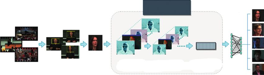
Computational Intelligence and Neuroscience 3

expression. They combined different modalities and per- technology, engineering, and mathematics) disci-
formed fusion at decision level and feature level, achieving plines have been collected.
better accuracies than single modality classifiers. Similarly, (iv) A new research domain was introduced by pro-
in [42], a multitask global-local network (MGLN) is pro- posing a method of utilizing instructor’s facial ex-
posed for facial expression recognition which combines pressions in a classroom environment using
two modules: a global face module (GFM) which extracts computer vision techniques.
spatial features from the frame having peak expression and
a part-based module (PBM) which learns temporal features The rest of the paper is organized as follows. In Section 2,
from eyes, mouth, and nose regions. Extracted features of the proposed methodology for instructor’s expression rec-
GFM through a CNN and PBM through a long short-term ognition is presented. To evaluate the proposed method-
memory (LSTM) network are then fused together to ology, the experimental results are presented in Section 3.
capture robust facial expression variation. In [43], a shallow Section 4 concludes with a summary of the achievements of
CNN architecture is proposed with dense connectivity the proposed method.
across pooling while dropping the fully connected layer to
enforce feature sharing. Under limited training data, it 2. Proposed Methodology
achieves good performance for the effective representation
 The general framework of the proposed facial expression
of facial expressions, but the pretrained DenseNet40 and
 recognition system is presented in Figure 1. Its first step
DenseNet121 show performance degradation due to
 involves face detection of an instructor from the lecture
overfitting. To combat the challenges of limited data in the
 videos. The extracted instructor’s face frames are then
domain of deep learning, a method presented in [33] in-
 subjected to key frame extraction where redundant frames
troduces novel cropping and rotation strategies to make
 are discarded and only midframes are kept for each ex-
data abundant as well as useful for feature extraction using
 pression. These key frames are further processed to extract
a simplified CNN. The cropping and rotation method
 deep features from different layers of a CNN. Then, these
removes redundant regions and retains useful facial in-
 extracted deep features are used to train an RELM classifier
formation, and the results on CK+ and JAFFE are
 for recognizing instructor’s facial expressions within five
competitive.
 classes. RELM is one of the variants of the extreme learning
 The perception of information processing has com-
 machine (ELM), which is based on a structural risk mini-
pletely changed by these deep learning approaches. Due to
 mization principle. The structural risk minimization prin-
its remarkable ability of self-learning, deep learning is
 ciple is used to optimize the structure of ELM, and
considered to be a better option for vision and classification
 regularization is utilized for accurate prediction. This
problems [44]. Other approaches for classification include
 principle is effective in improving the generalization of ELM.
pretrained networks which reduce the process of long
 These steps are further explained in the following sections.
training by introducing the use of pretrained weights [45].
However, learning here involves tuning of millions of
network parameters and huge labeled data for training. Since 2.1. Face Detection and Key Frame Selection. Recognizing an
FER is significantly relevant to a number of fields, we believe instructor’s facial expressions is challenging because it is
FER using deep features can be applicable in understanding different from the conventional facial expression recognition
the semantics of instructor’s facial expressions in a class- system. Essentially, the data are acquired in a classroom
room environment. environment. This involves challenges like face invisibility,
 The model proposed here aims to automate the recog- e.g., when the instructor is writing on the board, occlusion,
nition of an instructor’s facial expression by incorporating e.g., when the instructor is reading the slide from the laptop
visual information from lecture videos. Automatic assess- and half of the face is hidden behind the screen, and varying
ment of instructors through emotion recognition may im- lightening conditions, e.g., when the instructors walk under
prove their teaching skills. Such an assessment mechanism the projector’s light. The proposed algorithm is designed in
can save time and resources which are currently utilized to such a way so as to overcome such challenges. Keeping in
fill up bundles of survey forms. view the indoor and single object environment, faces of
 The main contributions of this paper are as follows: instructors are detected using the Viola–Jones face detection
 approach [46]. The detection of faces in an image by Vio-
 (i) A novel feedforward neural network has been
 la–Jones algorithm sought full upright frontal faces that also
 proposed for instructor’s facial expression recog-
 reduce the nonfacial expression frames [47]. For robust
 nition, which is fast and robust.
 practical detection, the face must be visible to the camera;
 (ii) The proposed fast feedforward-based technique can hence, only frontal faces are considered. Once the face is
 learn deep neural features from any type of con- detected, the bounding box around the face of the instructor
 volutional neural networks. is cropped, to form a region of interest. According to the
 (iii) A new dataset of instructor’s facial expressions in literature, the main step in processing videos is to segment
 classroom environments has been produced. Online the video into temporal shots. A shot consists of a sequence
 lecture videos of instructors delivering lectures of frames. Among all the frames, a key frame provides salient
 encompassing a variety of STEM (science, information of the shot. It summarizes the content of the

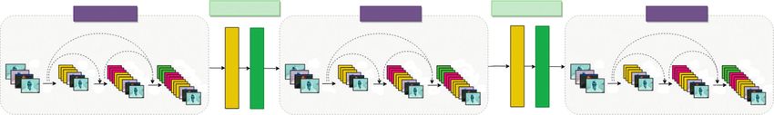
4 Computational Intelligence and Neuroscience

 Instructor emotion
 Deep neural network recognition
 architecture
 Instructor’s Face Key frame Awe
 lecture videos detection extraction RELM
 classifier Amusement

 Confidence

 Disappointment
 Convolutional Downsampled Feature vector
 feature maps pooling output (1∗x)
 Neutral

 Figure 1: Framework of the proposed instructor’s facial expression recognition.

video by removing redundant information and delivering representations, that does not ensure best accuracy. Instead
only significant condensed information. By utilizing shot of acquiring features from just the last layer, features are
boundary detection, we select the middle frame of the shot as extracted from convolution, pooling, and regularization
the key frame [48]. Generally, a human facial macro- layers. We have empirically evaluated the performance of
expression lasts for about half a second to four seconds [49]. various layers of deep networks in Section 3. From Den-
Thus, all the frames in this time span are considered. For seNet201, features are extracted using the
each expression, the first and last frames usually show a conv4 block9 1 bn layer. For AlexNet, GoogleNet, Incep-
neutral expression, while the middle frame gives a good tionv3, and ResNet50 features are extracted from drop7,
expression representation of the shot. Middle frames for pool5 drop 7x7 s1, activation 94 relu, and avg pool, re-
each expression label are therefore selected as shown in spectively. For ResNet101 and ResNet18, we opted for pool5.
Figure 2. Using this key frame selection procedure, re- The DenseNet architecture has been designed aiming at a
dundant frames are narrowed down to only the limited maximum flow of information between layers in the net-
frames which show the peak expression. In expression work. All layers are directly connected with each other, and
representation, only those frames are selected that best each layer receives feature maps produced by all preceding
characterize the emotion. Frames exhibit different levels of layers, which then transfers into succeeding layers. Unlike
expressiveness. When a person expresses an emotion, a ResNets, here features are combined by concatenation rather
transition from a neutral to maximum expression occurs than summation before passing into a layer. Hence, the lth
which is known as apex [50]. Training a deep learning al- layer has l inputs, consisting of the feature maps of all
gorithm on every single frame may negatively impact preceding convolutional blocks. Its own feature maps are
classification accuracy. Hence, for training, we select frames passed on to all L − 1 subsequent layers. So in an L-layer
that contain the apex of an expression because of their strong network, there are L(L + 1)/2 direct connections unlike
expression content while discarding the frames where the traditional architectures which have L number of connec-
subject is neutral for that emotion [51]. These key frames are tions. The lth layer receives the featuremaps xl of all pre-
targeted to identify five emotions: amusement, awe, confi- ceding layers, x0, . . . , xl− 1 , which is in the following form:
dence, disappointment, and neutral.
 xl � Hl x0 , x1 , . . . , xl− 1 , (1)

2.2. Feature Extraction Using CNN Models. After acquiring where x0 , x1 , . . . , xl− 1 are the concatenation of the feature
the key frames, a deep feature representation of facial ex- maps in layers 0, . . . , l − 1th layer. Hl(.) is a composite
pressions is generated from a 2D-CNN. These deep learning function comprised of three operations which are batch
models have layered architecture that learns features at normalization (BN) [57], a rectified linear unit (ReLU) [58],
different layers (hierarchical representations of layered and a 3 ∗ 3 convolution (Conv). In traditional deep CNNs,
features). This layered architecture allows extracting high- layers are followed by a pooling layer that reduces feature
level, medium-level, and low-level features of an instructor’s maps size to half. Consequently, the concatenation opera-
face. Two types of networks are investigated: sequential tion used in equation (1) would be erroneous due to the
network and directed acyclic graph (DAG) [52]. A serial change in feature maps. However, downsampling layers are
network has layers arranged sequentially such as in AlexNet an essential part of convolutional networks. To facilitate
[45], which takes 227 × 227 2-dimensional input and has 8 consistent downsampling, DenseNets are designed so as to
layers. On the other hand, a DAG network has layers in the divide the network into multiple densely connected dense
form of directed acyclic graph, with multiple layers pro- blocks and transition layers are introduced [59]. Figure 3
cessing in parallel for yielding efficient results. Example shows transition layers consisting of convolution and
models of DAG are GoogleNet [53], DenseNet201 [54], pooling layers, present between dense blocks. The instructor
ResNet50, ResNet18, ResNet101 [55], and Inceptionv3 [56] feature maps are extracted from the layer
having depth of 22, 201, 50, 18, 101, and 44 layers, re- conv4 block9 1 bn which is connected to convolution layer
spectively. Although deeper layers have high-level feature conv4 block9 1 conv[0][0]. Because of this dense

Computational Intelligence and Neuroscience 5

 Figure 2: Representation of selected middle key frame for the expression of “amusement” from the shot of nine frames.

 Transition layer 1 Transition layer 2
 Dense block 1 Dense block 2 Dense block 3

 Convolution

 Convolution
 Pooling

 Pooling
 x0 x1 x2 x3 x0 x1 x2 x3 x0 x1 x2 x3
 x0 x1 x2 x0 x1 x2 x0 x1 x2
 x0 x1 x0 x1 x0 x1
 h1 h2 x0 h1 h2 x0 h1 h2 x0
 h3 h3 h3

Figure 3: DenseNet architecture with three dense blocks and adjacent transition layers. The solid lines represent the concatenation of
previous feature maps. The dashed lines show the connection of different layers.

connectivity, DenseNet requires fewer parameters as there is can approximate n distinct training samples with zero error,
no need to relearn redundant feature maps, as is the case in i.e.,
traditional convolutional networks. N � ��
 �
 ���oq − tq ��� � 0, (3)
 i�1
2.3. Classification by Regularized Extreme Learning Machine
(RELM). In this work, RELM [60] is investigated, to rec- then there must exist wi , bi and βi which satisfy the function:
ognize instructor’s emotions in classroom environments.
The extracted 2D-CNN features of an instructor’s facial 
 N 
 N

emotions are fed to an RELM classifier for predicting among βi gi xq � βi gi wi · xq + bi � tj , j � 1, . . . , N.
 i�1 i�1
five emotion classes. ELM is a single hidden layer feedfor-
ward neural network (SLFN), having fast training speed and (4)
good generalization performance. However, it tends to cause The above equation can be written as
overfitting as it is based on the principle of empirical risk
minimization (ERM) [61]. To overcome that drawback, Hβ � T, (5)
RELM was introduced, which is based on structural risk
minimization (SRM) [62]. The ERM is based on the sum of where H(w1 , w2 , . . . , wi , b1 , b2 , . . . , bi , x1 , x2 , . . . , xi , )
squared error of the data samples. Having fewer data g w1 · x1 + b1 . . . g wn · x1 + bN 
samples and small empirical risk gives less training error for ⎡⎢⎢⎢ ⎤⎥⎥⎥
training data but large testing error for unseen data, causing � ⎢⎢⎢⎢⎣ ... ... ... ⎥⎥⎥,
 ⎥⎦ (6)
overfitting. Therefore, RELM works on the SRM principle g w1 · xN + b1 . . . g wn · xN + bN 
which is based on the statistical learning theory. It provides
the relationship between empirical risk and real risk, which where H denotes the hidden layer output matrix of network.
is known as the bound of the generalization ability [63]. Traditionally, the parameters of hidden nodes are iteratively
Here, the empirical risk is represented by the sum of squared adjusted in order to reach the optimal minima. In contrast,
error, i.e., ‖ε‖2 and structural risk can be represented with to train an SLFN, we can arbitrarily select hidden node
‖β‖2 . parameters with any nonzero activation function and can
 Specifically, there are n distinct training samples determine the output weights analytically. Hence, for finding
(xi , ti )εRk ∗ Rm with g(x) as the activation function. For the the output matrix in reference to the theory of least squares,
ith samples, the RELM with hidden nodes N is modeled as the estimation of β can be written as
 
 N 
 N β � H† T, (7)
 βi gi xq � βi gi wi · xq + bi , (2)
 i�1 i�1 where H† is known as the generalized inverse of H also called
 as Moore–Penrose generalized inverse.
where w � [wi1 , wi2 , . . . , wm ]T is the weighted vector which Here, the aim of the RELM algorithm is to find an
shows the connection among hidden nodes and input nodes. optimum solution β for satisfying the following equation:
β � β � [βi1 , βi2 , .., βi ]T represents weighted output which
 2
maintains the connection between hidden nodes to the ‖Hβ − T‖F � minβ ‖Hβ − T‖2F , (8)
output nodes and bi is the bias of hidden layer nodes. The
value wi · xq represents the inner product and where ‖ · ‖F is known as Frobenius norm. There are a
O � [oj1 , oj2 , .., ojN ]T represents the output vector which is number of regularization techniques reported in the liter-
m × 1. So typically, if a standard SLFN with N hidden nodes ature such as minimax concave [64], ridge regression, and

6 Computational Intelligence and Neuroscience

nonconvex term [65]. These terms have been utilized for mathematics) domains as their applications empower stu-
linear systems to reduce the overall variance. However, when dents for innovative work in this technology-driven era.
the number of hidden nodes for ELM exceeds the value 5000, There are a total number of 30 actors and 30 corresponding
it starts to overfit the model. By taking the advantage that the videos with different time durations, from 20 minutes to 1
linear system of these SLFN’s output can be calculated hour. To maintain some diversity, 23 are male instructors
analytically, we use the Frobenius norm for regularization. and 7 are female instructors. In each category of expressions,
Equation (8) can be written as follows: a total of 425 images are present, to ensure that classes are
 2 balanced. The frame resolution of each video varies from
 ‖Hβ − T‖F � minβ ‖Hβ − T‖2F + λ‖β‖2F , (9) 368 × 290 to 1280 × 720 pixels with 30 frames per second.
 Five expression categories for instructors are identified,
 −1
 β � HT H + λI HT T. (10) namely, amusement, awe, confidence, disappointment, and
 neutral. Table 1 shows a tabular view of the instructor’s
 For regularized ELM, β is calculated as shown in expression dataset.
equation (10) where λ is the regularization factor. When the The dataset is constructed from the lecture videos of the
term λ is a positive constant term (i.e., > 0), equation (10) real classroom in a realistic environment. The subjects under
gives the optimal solution of equation (9). By regulating λ, consideration are real-life instructors having experienced
the proportion of empirical risk and structural risk can be and shown emotions while delivering the session. While
adjusted. The optimal trade-off between these two risks will dealing with students, instructor’s experience and express
make a generalized model. The working of the proposed emotions from pleasure to disappointment and anger [69].
RELM scheme is summarized by the algorithmic steps as They gradually develop different schemes to regulate their
shown in Figure 4. genuine emotions [70]. In [69], instructors admitted to
 controlling the intensity of unpleasant emotions such as
3. Experimentation Results and Discussion anger. However, the majority of the literature demonstrates
 the authentic display of emotions allowing instructors to
3.1. Experimental Setup. For the experimentation, MATLAB display emotion in a controlled fashion [71]. In accordance
2018 has been used on an Intel Core i5 machine with 16 GB with the literature and our targeted environment, we con-
RAM and an NVIDIA TITAN XP GPU. For the evaluation structed a category which could be a representative of both
of the proposed framework, four standard metrics of pre- anger and disgust. Important expressions such as anger are
cision, recall, F1-score, and accuracy have been used. The considered under the category of “disappointment,” as these
validation schemes used for evaluating the technique are 10- expressions are mild in the university’s classroom envi-
fold cross-validation, leave-one-actor-out (LOAO), leave- ronment. Research [72] has shown a slight decrease in the
one-sample-out (LOSO), and data split schemes (70–30%). expressiveness of instructor’s unpleasant emotions such as
These validation techniques define the division of training anger, anxiety, and transforming into a form that is “dis-
and testing sets. For example, in the 10-fold, the data are split appointment and disgust”. Here, it is useful to note that
into 10 folds where 9 folds are used to train the model and disappointment frequency was five times more than the
the remaining fold is used for testing and the average ac- sadness frequency. In the proposed methodology, after
curacy is recorded. The process iterates until each fold of the thorough research, we intended to focus on the emotions
10 folds has been used for testing. Similarly, for LOAO, that are conceptually salient and distinct in an academic
expression samples for all actors but one are used for environment. Twenty annotators including instructors and
training. Then, testing is done using images for the unseen students evaluated the facial expression of instructors, and
actor. The iteration occurs for all the actors one by one. In labels were assigned on the basis of majority voting.
LOSO, all the samples for training are considered except one
used as a testing sample.
 3.2.2. Cohn–Kanade. The CK dataset [66] consists of video
3.2. Datasets for Facial Expression Recognition. The proposed sequences of 97 subjects showing six expressions with a total
model is evaluated on four different expression datasets, of 582 images. Basic expressions are anger, contempt, fear,
first, on a new Instructor Expression Video (IEV) dataset, disgust, happiness, surprise, and sadness. Image resolution is
created by the authors. To evaluate and explore the gener- 640 × 480 pixels. Sequences start with the neutral expression
alization of the proposed approach, three benchmark facial up to the last frame showing the emotion for that particular
expression datasets are also explored: the Cohn–Kanade label. Sample images for every expression are shown in
(CK) facial expression dataset [66], Japanese Female Facial Figure 5.
Expression (JAFFE) dataset [67], and the Facial Expression
Recognition 2013 (FER2013) dataset [68].
 3.2.3. Japanese Female Facial Expression (JAFFE). The
 JAFFE [67] database includes 213 images of 10 different
3.2.1. IEV Dataset. In this new dataset, lecture videos are female actors posing for seven facial expressions. Six of them
acquired from multiple open course-ware websites from are basic expressions: anger, joy, sadness, neutral, surprise,
top-ranked universities around the globe. We have incor- disgust, and fear plus one neutral as shown in Figure 6.
porated the STEM (science, technology, engineering, and Image resolution is 256 × 256 pixels.

Computational Intelligence and Neuroscience 7

 Algorithmic steps
 Given a set of deep neural features x, target output t, an activation function g (x) with N number of hidden
 nodes. the weight vector, w connects the hidden node with the output nodes.
 Step 1:assign the input weights and the bias of hidden layer nodes B randomly (wi, bi), i = 1, 2, ..., L.
 Step 2:compute output matrix H (w1, ..., wL, x1, ..., xN, b1, ..., bL)
 Step 3:compute output weights: β = HTT.
 ~
 Step 4:for regularization the output term is computed by using β = (λ + HTH)–1 HTT
 Return: parameters β, W, and b.
 Figure 4: The RELM algorithm for classification.

 Table 1: Tabular view of the new Instructor Expression Video (IEV) dataset along with sample images for each expression class.
Sample images from lecture videos Expression No. of samples Gender

 Amusement 425

 Awe 425

 Male: 23
 Confidence 425 Female: 7

 Disappointment 425

 Neutral 425

 Figure 5: Sample sequence of seven expressions from the CK dataset.

 Figure 6: Sample images taken for each expression from the JAFFE dataset.

3.2.4. FER2013 Dataset: Facial Emotion Recognition (Kaggle). challenging aspect of this dataset is variations in images,
Facial Expression Recognition 2013 (FER2013) database [68] pose, partial faces, and occlusion with the use of hands.
was introduced in the International Conference on Machine
Learning (ICML) Workshop on Challenges in Representa-
tion Learning. FER2013 dataset consists of a total of 35,887 3.3. Feedforward Network Tuning with Number of Nodes for
grayscale images of 48 × 48 resolution; most of them are in Seven Convolutional Models. RELM assigns the initial input
wild settings. It was created by using the Google image weights and hidden biases randomly. Through a generalized
search API to scrape images through keywords that match inverse operation, the output weights of SLFNs are deter-
emotion labels. FER2013 has seven emotion classes, namely, mined analytically. However, there are parameters like the
angry, disgust, fear, happy, sad, surprise, including neutral as selection of the number of hidden nodes which have to be
shown in Figure 7. In contrast to the posed datasets, the tuned to reduce classification error [73]. For tuning the

8 Computational Intelligence and Neuroscience

 Figure 7: Sample images taken for each expression from the FER2013 dataset.

 1
 0.9
 Recognition accuracy on CK

 0.8
 0.7
 0.6
 0.5
 0.4
 0.3
 0.2
 0.1
 0
 100 500 1000 2000 3000 4000 5000 8000 10000 20000
 Number of ELM hidden nodes

 AlexNet ReseNet101
 DenseNet201 Inceptionv3
 GoogleNet
Figure 8: Impact of the number of nodes on expression recognition performance of the convolutional neural models on the CK dataset.

hyperparameters for optimization of the proposed algo- FER2013 dataset, an upward trend is observed as the number
rithm, a grid search approach with the range of [10–100000] of nodes increases from 5000 to 10,000 as shown in Fig-
has been adopted. Figure 8 represents the hidden node ure 11. In contrast to the other three datasets, FER2013
behavior for five 2D-CNN networks, namely, DenseNet201, shows better performance on 10000 nodes instead of 5000.
AlexNet, ReseNet101, GoogleNet, and Inceptionv3 on the As the number of nodes increases up to 20000, the accuracy
CK dataset. remains the same or decreases, but the training time doubles.
 It has been observed from Figure 8 that DenseNet201 Hence, after the empirical selection of the number of hidden
and AlexNet performed better emotion recognition among nodes, these parameters will remain the same for the rest of
all the five deep networks. In the case of GoogleNet, we the experiments.
observe a consistent trend of up to 5000 nodes followed by
an abrupt decrease in accuracy up to 20,000 nodes. Similarly,
Inceptionv3 started from very low accuracy, increased up to 3.3.1. Empirical Analysis of Deep Neural Features on Stan-
5,000, remained constant for 8000 and 10,000 nodes, and dard Datasets and IEV Dataset. Empirically, seven 2D-CNN
eventually showed a decrease in accuracy at 20,000. For models are evaluated here, namely, AlexNet, DenseNet201,
ResNet101, initially the trend is inconsistent, followed by a ReseNet18, ReseNet50, ReseNet100, GoogleNet, and
steady fall after 4,000 nodes. However, DenseNet201 showed Inceptionv3 on two standard datasets and on the new IEV
a persistent increase from 100 up to 5,000 without fluctu- dataset. For evaluation of the proposed model, high-di-
ations. It decreases the accuracy for the next two values and mensional feature maps are extracted from all seven models,
showed the same amount of accuracy on 20,000 as of 5,000 for each dataset. To visually examine the behavior, a bar
nodes. A similar trend is observed in the case of AlexNet chart is shown in Figure 12. It can be seen that ResNet18
with just a slight increase at 20,000 nodes rather than a gives the least accuracy among its variants followed by
decrease. AlexNet initially showed good results in com- Inceptionv3 and GoogleNet. A possible reason for the poor
parison with DenseNet201, but with the increase in the accuracy of ResNet18 is the presence of an excessive number
number of nodes, DenseNet201 outperformed AlexNet. To of parameters, and hence, every layer has to learn weights
ensure the best model performance, this experiment has accordingly. In contrast, DenseNet201 outperforms other
been performed to select an optimal number of nodes. On models as it has 3 times less parameters than ResNet for the
average, the optimal number of RELM nodes for all three same number of layers. Its narrow layers add only fewer
datasets is 5000 nodes for all the five models. For Jaffe, only feature maps in network collection and the classifier makes
the top two 2D-CNN models showing better performance decisions accordingly.
are selected as shown in Figure 9. A similar behavior is Table 2 presents a tabular view of these models showing
observed for the IEV dataset as shown in Figure 10. For the the statistical performance of the same experiment.

Computational Intelligence and Neuroscience 9

 1
 0.9
 0.8

 Recognition accuracy
 0.7
 0.6
 0.5
 0.4
 0.3
 0.2
 0.1
 0
 100 500 1000 2000 3000 4000 5000 8000 10000 20000
 Number of hidden nodes

 DenseNet201
 AlexNet
 Figure 9: Expression recognition performance of DenseNet201 and AlexNet on the JAFFE dataset for different number of nodes.

 0.9
 Recognition accuracy

 0.85
 0.8
 0.75
 0.7
 0.65
 0.6
 0.55
 0.5
 1000 2000 5000 10000 20000
 Number of hidden nodes
 AlexNet
 DenseNet201
Figure 10: Expression recognition performance of DenseNet201 and AlexNet on the Instructor Expression Video (IEV) dataset with an
increase in the number of nodes.

 0.8
 Recognition accuracy

 0.6
 0.4
 0.2
 0
 5000 10000 20000
 Number of hidden nodes

 AlexNet
 DenseNet201
Figure 11: Expression recognition performance of DenseNet201 and AlexNet on the FER2013 dataset with increase in the number of nodes.

Conventionally, the final fully connected layer is normally Evaluation parameters for network models across corre-
used for feature extraction, but experiments are performed sponding layers are listed in Table 2.
on various layers and it is observed that some layers out- Performance is evaluated on three validation schemes
perform the fully connected layer’s accuracy. DenseNet 10-fold, split (70–30%), LOAO, and LOSO. Table 3 shows
“convolutional layer” and AlexNet “drop7” give the best the results using the abovementioned layers of DenseNet201
accuracy of 85% and 83%, respectively. Similarly, and AlexNet on three standard datasets (Jaffe, CK, and
ResNet101’s pool5 layer and GoogleNet’s layer “pool5_- FER2013) across all three schemes. On the Jaffe dataset, best
drop_7∗7_sl” give the best accuracy of 84% and 81%. accuracy is achieved with DenseNet201. For schemes of split

10 Computational Intelligence and Neuroscience

 1

 0.9

 0.8

 Achieved classification accuracy
 0.7

 0.6

 0.5

 0.4

 0.3

 0.2

 0.1

 0
 ResNet18 ResNet50 ResNet101 Inceptionv3 GoogleNet Alexnet DenseNet201

 Cohn-Kanada
 JAFFE
 IEV

Figure 12: Accuracy of seven 2D-CNN models (AlexNet, DenseNet201, ReseNet18, ResNet50, ResNet100, GoogleNet, and Inceptionv3)
across CK, Jaffe and IEV datasets for facial expression recognition.

Table 2: Statistical performance of seven 2D-CNN models (AlexNet, DenseNet201, ReseNet18, ResNet50, ResNet100, GoogleNet, and
Inceptionv3) on the Instructor Expression Video (IEV).
Network Layer Accuracy Neurons Precision Recall F1-score Error
DenseNet201 conv4_block9_1_bn 0.85 5000 0.85 0.87 0.85 0.14
AlexNet drop7 0.83 5000 0.83 0.85 0.83 0.12
GoogleNet pool5-drop_7 × 7_s1 0.81 5000 0.81 0.83 0.81 0.18
Inceptionv3 activation_94_relu 0.78 5000 0.75 0.79 0.76 0.22
ResNet101 pool5 0.84 5000 0.83 0.85 0.83 0.16
ResNet18 pool5 0.75 5000 0.79 0.81 0.79 0.2
ResNet50 avg_pool 0.82 5000 0.82 0.82 0.82 0.82

Table 3: Results of deep model layers on standard datasets (CK, Jaffe, and FER2013) using validation schemes across RELM classifier.
Dataset Network Layer Split (70–30%) 10-fold LOAO LOSO
 DenseNet201 conv4_block9_1_bn 96.8 92.44 93.4 94.55
Jaffe
 AlexNet drop7 91.67 86.03 84.01 85.91
 DenseNet201 conv4_block9_1_bn 86.59 80.5 81.59 81.99
CK
 AlexNet drop7 81.67 86.03 84.01 85.91
 DenseNet201 conv4_block9_1_bn 62.74 — — —
FER2013
 AlexNet drop7 45.91 — — —

(70–30%), 10-fold cross-validation, LOAO, and LOSO, the 92.0%, 90.2%, and 81.3%, respectively. It is validated with a
accuracies are 96.8%, 92.44%, 93.4%, and 94.55%, respec- 70–30% split validation scheme. Furthermore, on all four
tively. Similarly, results for the CK dataset are 86.59%, datasets, namely, CK, Jaffe, FER2013, and IEV, the total
80.5%, 81.59%, and 81.99% on schemes of split (70–30%), inference time taken is calculated across ELM and RELM
10-fold cross-validation, LOAO, and LOSO, respectively. classifiers as shown in Table 4. For Jaffe and CK, RELM
For the FER2013 dataset, DenseNet201 and AlexNet give outperforms ELM giving 0.7 s instead of 1.1 s and 21.8 s
accuracy of 62.74% and 45.91%, respectively. rather than 30.1 s, respectively. FER2013 worked best on
 Figure 13 shows the confusion matrix obtained by 10000 nodes; however, the training time exceeds for RELM
RELM and ELM on the IEV dataset. It shows that, with to 51.03 s and 17.44 s in the case of ELM. For the IEV
RELM, the per-class accuracy for amusement, awe, con- dataset, it gives 21.28 s for ELM and 13.94 s for RELM, a
fidence, disappointment, and neutral is 86.3%, 90.8%, difference of 7.34 s.

Computational Intelligence and Neuroscience 11

 Accuracy: 84.13% Accuracy: 88.10%

 83.7% 3.4% 1.6% 2.2% 7.6% 86.3% 2.5% 2.4% 1.5% 4.1%
 Amusement Amusement
 108 4 2 3 9 13 3 3 2 5

 5.4% 84.0% 2.3% 0.7% 12.6% 3.8% 90.0% 0.0% 1.5% 8.9%
 Awe Awe
 7 100 3 1 15 5 108 0 2 11
 Output class

 Output class
 2.3% 0.0% 89.9% 1.5% 4.2% 2.3% 0.8% 92.0% 1.5% 4.1%
 Confidence Confidence
 7 100 3 2 5 3 1 115 2 5

 0.0% 2.5% 2.3% 88.1% 1.7% 0.0% 3.4% 0.8% 90.2% 1.6%
 Disappointment Disappointment
 0 3 3 118 2 0 4 1 119 2

 8.5% 10.1% 3.9% 7.5% 73.9% 7.6% 2.5% 4.8% 5.3% 81.3%
 Neutral Neutral
 11 12 5 10 88 10 3 6 7 100
 Amusement

 Awe

 Confidence

 Disappointment

 Neutral

 Amusement

 Awe

 Confidence

 Disappointment

 Neutral
 Precision 0.839373 Target class Precision 0.880936 Target class
 (a) (b)

 Figure 13: Confusion matrix of RELM and ELM on Instructor Expression Video (IEV) dataset.

 Table 4: Execution time taken (s) for CK, Jaffe, FER2013, and IEV across both classifiers.
 Training time (s) Testing time (s)
Database
 ELM RELM ELM RELM
Jaffe 1.11 0.749 0.06 0.02
Cohn–Kanade 30.17 21.83 0.48 0.27
FER2013 17.44 51.03 0.21 0.37
IEV 13.94 21.28 0.28 0.17

3.3.2. Performance Comparison of Single-Layer Feedforward other state-of-the-art techniques on Jaffe, CK, FER 2013,
Network (ELM and RELM) with Traditional Classifiers. and IEV datasets is compared and illustrated in Table 6.
The performances of ELM and RELM classifier across tradi- Given that it is not always possible to replicate algo-
tional classifiers are empirically evaluated, as shown in Table 5. rithms from published results, for fair comparisons, we
To examine the behavior, the whole framework is fixed and have used the same validation approach scheme used by
only the classifier in the classification part is changed. Features each method, so findings are categorized on the basis of
from five 2D-CNN models are extracted, and across every set of the validation scheme used. For JAFFE, 10-fold cross-
features, the estimated strength of ELM and RELM is tested on validation results gave 92.4% accuracy outperforming the
CK. Analysing the trend, least performance is shown by Naı̈ve kernel-based isometric method [84], CNN method [74],
Bayes and decision tree across all the models. However, support and autoencoders [76] which are 81.6%, 90.37%, and
vector machine (SVM) outperformed all the conventional 86.74%, respectively. For a 70–30 split, the proposed
classifiers. ELM and RELM show visible performance gains approach gave 96.8% whereas representational autoen-
over all the models in comparison with ten different classifiers. coders [85] and CNN [77] lag behind. A similar situation
ELM, contrary to the conventional backpropagation algorithm, occurs for the other two schemes as well. However, for
is based on empirical risk reduction technique and needs only the CK dataset, 82% is achieved for 10-fold cross-vali-
one iteration for its learning process. This property has made dation whereas DTAN and DTGN [75] outperform the
this algorithm have fast learning speed and good generalization method here with 91.4%. Similar results are observed for
performance yielding optimal and unique solution. For RELM, other validation schemes. We found the reason behind
the regularization term helps in reducing overfitting without less accuracy on CK is low variance among the facial
increasing computational time making a generalized instructor expressions and low-resolution grayscale images. In the
expression prediction model. case of FER-2013, the literature shows an overall low
 trend in accuracy because of high variance and occlusion
 conditions of the dataset. Wang et al. [79] performed
3.3.3. Comparison with State of the Art. In this section, the multiple methods in which HOG with C4.5 classifier gave
performance of the proposed technique as compared to 46.1% and CNN with decision tree gave 58.8% accuracy.

12

 Table 5: Comparison of ELM/RELM with the traditional classifiers on the CK dataset.
 AlexNet DenseNet GoogleNet Inceptionv3 ResNet101
Classifiers
 Accuracy Precision F1-score Accuracy Precision F1-score Accuracy Precision F1-score Accuracy Precision F1-score Accuracy Precision F1-score
RELM 0.82 0.80 0.83 0.83 0.85 0.82 0.78 0.75 0.78 0.78 0.69 0.74 0.82 0.84 0.82
ELM 0.83 0.79 0.82 0.73 0.75 0.74 0.72 0.76 0.70 0.78 0.79 0.79 0.56 0.46 0.52
SVM 0.80 0.80 0.81 0.77 0.75 0.77 0.80 0.80 0.80 0.77 0.75 0.77 0.82 0.82 0.80
Naı̈ve Bayes 0.23 0.25 0.25 0.20 0.28 0.25 0.29 0.28 0.28 0.24 0.25 0.24 0.43 0.45 0.45
Random forest 0.45 0.49 0.46 0.76 0.79 0.75 0.53 0.48 0.52 0.52 0.53 0.52 0.70 0.77 0.75
K-nearest neighbors 0.57 0.59 0.56 0.60 0.68 0.69 0.60 0.60 0.61 0.53 0.54 0.59 0.79 0.79 0.77
Logistic regression 0.29 0.31 0.29 0.53 0.52 0.52 0.55 0.59 0.56 0.58 0.60 0.59 0.59 0.60 0.61
Random tree 0.26 0.28 0.25 0.53 0.55 0.50 0.75 0.75 0.73 0.57 0.57 0.57 0.55 0.53 0.57
Simple logistic 0.48 0.47 0.48 0.73 0.74 0.70 0.73 0.75 0.75 0.75 0.78 0.75 0.74 0.74 0.74
Decision table 0.23 0.20 0.23 0.48 0.45 0.46 0.74 0.70 0.74 0.43 0.45 0.40 0.42 0.42 0.42
Multiclass classifier 0.57 0.62 0.60 0.65 0.67 0.67 0.68 0.74 0.70 0.74 0.74 0.74 0.70 0.74 0.70
Multilayer perceptron 0.43 0.43 0.41 0.65 0.70 0.69 0.78 0.68 0.67 0.68 0.65 0.66 0.65 0.68 0.68
 Computational Intelligence and Neuroscience

Computational Intelligence and Neuroscience 13

 Table 6: Accuracy comparison between state-of-the-art approaches on JAFFE, CK, and FER2013.
Dataset Validation scheme Methods Accuracy (%)
 KDIsomap [74] 81.6
 EDL [75] 90.3
 10-fold
 CBIN [76] 86.7
JAFEE Proposed approach 92.4
 RAU’s [46] 86.3
 Split (70–30%) CNN [77] 76.5
 Proposed approach 96.8
 DTAN + DTGN [31] 9 .4
 10-fold DNN [22] 90.9
CK Proposed approach 82.8
 DCNN as SCAE [78] 92.5
 Split (70–30%)
 Proposed approach 86.5
 HOG + C4.5 [79] 46.1
 CNN [80] 57.1
 CNN + decision tree [79] 58.8
FER2013 Split (70–30%) VGG-Face + FR-Net-A + B + C + Audio [81] 60.0
 AlexNet [82] 61.0
 CNN ensemble [83] 62.4
 Proposed approach 62.7

 Table 7: Accuracy comparison between convolution neural networks on standard datasets along with time taken per frame.
CNN model JAFFE (%) CK (%) FER2013 (%) Time taken per frame (sec) Number of parameters (million)
AlexNet [86] 93 90.2 61.1 — 61
VGG16 [86] 96 92.4 59.6 0.94 138
VGG19 [87] 93 93 60 — 144
ResNet101 [88] 90 — 49 — 44.5
Inceptionv3 [89] 75.8 76.5 — — 23
Proposed method 96.8 86.5 62.5 0.74 0.005

From exploring CNN [80] to AlexNet [82] and then to shows results in 0.2% less time duration on Jaffe. These
CNN ensemble [83], an increasing trend from 57.1%, pretrained models work on backpropagation approaches
61.0%, and 62.4% is observed, respectively. In [81], VGG where the weights are updated after every iteration. In
is incorporated with face recognition models trained on contrast, the proposed feedforward model decreases the
large dataset and audio features give 60% accuracy. The computational time, making it fast to learn and classify the
proposed method outperformed other state-of-the-art instructor’s expressions in classroom.
methods on Jaffe. This feedforward approach combined Our algorithm not only performs well on the annotated
with strong classifier forms a generalized feedforward datasets but also demonstrates the implementation on the real-
neural model for instructor expression recognition. time video stream generated through webcam or any other
 source by framewise traversing. The face detection and key
 frame extraction blocks in the proposed framework clearly
3.3.4. Comparison with Pretrained Convolutional indicate how to handle the real-time video data to be used for
Approaches. Table 7 presents a comparison of accuracy facial expression in subsequent stages. For real-time results and
along with execution times taken by the pretrained con- to run the trained model on devices with low-computational
volutional neural models on three standard datasets: Jaffe, strength such as mobile phones, edge devices, or embedded
CK, and FER2013. CNN models AlexNet and VGG16 [86] architectures, TensorFlow Lite may be used. To implement in a
gave 93% and 96% on Jaffe, 90.2% and 92.4% on CK, and real-time environment captured through a webcam or
61.1% and 59.6% on FER2013, respectively, with an exe- smartphone, we only need to run an inference on embedded
cution time of 0.94 s. Similarly, ResNet101 shows 90% on devices or raspberry pi with an accelerator. At inference level,
Jaffe and 49% on FER2013, and Inceptionv3 [90] gives 75.8% testing is done frame by frame and an inference graph will be
on Jaffe and 76.5% on CK. Lastly, it is compared with the generated having confidences which could then be burned on
proposed model which gives 96.8% and 86.59% accuracy on the device as per requirement. In essence, these utilities provide
Jaffe and CK, respectively, with 0.74 s average execution time full-fledged feasibility for deploying the proposed application in
taken for each emotion per frame. The proposed model a real-time resource-constrained environment.

14 Computational Intelligence and Neuroscience

4. Conclusion [3] S. Hickson, N. Dufour, A. Sud, V. Kwatra, and I. Essa,
 “Eyemotion: classifying facial expressions in VR using eye-
In this paper, a novel approach has been proposed for facial tracking cameras,” in Proceedings of the 2019 IEEE Winter
expression recognition of instructors in a classroom envi- Conference on Applications of Computer Vision (WACV),
ronment by incorporating a feedforward learning model Waikoloa Village, HI, USA, January 2019.
with deep features. In contrast to backpropagation ap- [4] M. A. Assari and M. Rahmati, “Driver drowsiness detection
proaches, the proposed model works in a feedforward using face expression recognition,” in Proceedings of the 2011
 IEEE International Conference on Signal and Image Processing
fashion. It extracts the deep features from a neural model for
 Applications (ICSIPA), November 2011.
high-level representation gain, without updating the weights [5] T. Bai, Y. F. Li, and X. Zhou, “Learning local appearances with
iteratively, causing a reduction in computational time sparse representation for robust and fast visual tracking,”
complexity. Extensive experimentations are performed with IEEE Transactions on Cybernetics, vol. 45, no. 4, pp. 663–675,
state-of-the-art techniques, traditional classifiers, and other 2015.
deep neural models. The proposed method has proven to be [6] T. Chen and K. H. Yap, “Discriminative BoW framework for
successful in evaluating five instructor’s expressions in a mobile landmark recognition,” IEEE Transactions on Cyber-
classroom environment. For future research, we will in- netics, vol. 44, no. 5, pp. 695–706, 2014.
vestigate the performance of the model with more features [7] X. Zhu, X. Li, and S. Zhang, “Block-row sparse multiview
such as instructor’s speech and activity recognition ap- multilabel learning for image classification,” IEEE Transac-
proaches in order to improve the effectiveness of classroom tions on Cybernetics, vol. 46, no. 2, pp. 450–461, 2016.
 [8] K. Han, D. Yu, and I. Tashev, “Speech emotion recognition
teaching methods.
 using deep neural network and extreme learning machine,” in
 Proceedings of the Fifteenth Annual Conference of the Inter-
Abbreviations national Speech Communication Association, Singapore,
 September 2014.
FER: Facial expression recognition [9] R. J. J. Huang, Detection Strategies for Face Recognition Using
RELM: Regularized extreme learning machine Learning and Evolution, Citeseer, Princeton, NJ, USA, 1998.
IEV: Instructor Expression Video [10] B. Gökberk, A. A. Salah, and L. Akarun, “Rank-based decision
CNN: Convolution neural network fusion for 3D shape-based face recognition,” Lecture Notes in
SLFN: Single hidden layer feedforward neural network Computer Science, Springer, Berlin, Germany, pp. 1019–1028,
LOSO: Leave one sample out 2005.
LOAO: Leave one actor out. [11] W. Y. Zhao and R. Chellappa, “SFS based view synthesis for
 robust face recognition,” in Proceedings of the Fourth IEEE
 International Conference on Automatic Face and Gesture
Data Availability Recognition, Lille, France, May 2019.
 [12] T. Abegaz, G. Dozier, K. Bryant et al., “Hybrid GAs for Eigen-
The data used to support the findings of this study are based facial recognition,” in Proceedings of the 2011 IEEE
available from the corresponding author upon request. Workshop on Computational Intelligence in Biometrics and
 Identity Management (CIBIM), Paris, France, July 2011.
Conflicts of Interest [13] V. I. Pavlovic, R. Sharma, and T. S. Huang, “Visual inter-
 pretation of hand gestures for human-computer interaction: a
The authors declare that they have no conflicts of interest. review,” IEEE Transactions on Pattern Analysis and Machine
 Intelligence, vol. 19, no. 7, pp. 677–695, 1997.
 [14] R. Subramanian, J. Wache, M. K. Abadi, R. L. Vieriu,
Acknowledgments S. Winkler, and N. Sebe, “ASCERTAIN: emotion and per-
Muhammad Haroon Yousaf acknowledges the funding for sonality recognition using commercial sensors,” IEEE
 Transactions on Affective Computing, vol. 9, no. 2, pp. 147–
Swarm Robotics Lab under National Centre for Robotics and
 160, 2018.
Automation (NCRA), Pakistan. The authors also acknowl- [15] F. Cubukcu, “The significance of teachers’ academic emo-
edge the support from the Directorate of Advanced Studies, tions,” Procedia-Social and Behavioral Sciences, vol. 70,
Research and Technological Development (ASRTD) at the pp. 649–653, 2013.
University of Engineering and Technology, Taxila. [16] S. Prosen and H. S. Vitulić, “Emotion regulation and coping
 strategies in pedagogical students with different attachment
References styles,” Japanese Psychological Research, vol. 58, no. 4,
 pp. 355–366, 2016.
 [1] D. C. B. Silva, P. P. Cruz, A. M. Gutiérrez, and [17] E. Jensen, M. Dale, P. J. Donnelly et al., “Toward automated
 L. A. S. Avendaño, Applications of Human-Computer Inter- feedback on teacher discourse to enhance teacher learning,” in
 action and Robotics Based on Artificial Intelligence, Editorial Proceedings of the 2020 CHI Conference on Human Factors in
 Digital del Tecnológico de Monterrey, Monterrey, México, Computing Systems, pp. 1–13, Florence, Italy, April 2020.
 2020. [18] H. A. Hornstein, “Student evaluations of teaching are an
 [2] C.-H. Chen, I.-J. Lee, and L.-Y. Lin, “Augmented reality-based inadequate assessment tool for evaluating faculty perfor-
 self-facial modeling to promote the emotional expression and mance,” Cogent Education, vol. 4, no. 1, Article ID 1304016,
 social skills of adolescents with autism spectrum disorders,” 2017.
 Research in Developmental Disabilities, vol. 36, pp. 396–403, [19] H. W. Marsh, “Students’ evaluations of university teaching:
 2015. Dimensionality, reliability, validity, potential biases and