High-resolution mapping of circum-Antarctic landfast sea ice distribution, 2000-2018 - ESSD
←
→
Page content transcription
If your browser does not render page correctly, please read the page content below
Earth Syst. Sci. Data, 12, 2987–2999, 2020
https://doi.org/10.5194/essd-12-2987-2020
© Author(s) 2020. This work is distributed under
the Creative Commons Attribution 4.0 License.

           High-resolution mapping of circum-Antarctic landfast
                      sea ice distribution, 2000–2018
         Alexander D. Fraser1,2 , Robert A. Massom3,2 , Kay I. Ohshima4 , Sascha Willmes5 , Peter J. Kappes6 ,
                                   Jessica Cartwright7,8 , and Richard Porter-Smith2
              1 Institute for Marine and Antarctic Studies, University of Tasmania, Hobart, Tasmania, Australia
                2 Antarctic   Climate & Ecosystems Cooperative Research Centre, Hobart, Tasmania, Australia
                                  3 Australian Antarctic Division, Kingston, Tasmania, Australia
                   4 Institute of Low Temperature Science, Hokkaido University, Sapporo, Hokkaido, Japan
                              5 Dpt. Environmental Meteorology, University of Trier, Trier, Germany
                6 Oregon Cooperative Fish and Wildlife Research Unit, Department of Fisheries and Wildlife,

                                              Oregon State University, Corvallis, USA
                                        7 National Oceanography Centre, Southampton, UK
                            8 Ocean and Earth Science, National Oceanography Centre Southampton,

                                           University of Southampton, Southampton, UK
                              Correspondence: Alexander Fraser (alexander.fraser@utas.edu.au)

                                     Received: 22 April 2020 – Discussion started: 15 June 2020
                     Revised: 3 September 2020 – Accepted: 26 September 2020 – Published: 20 November 2020

       Abstract. Landfast sea ice (fast ice) is an important component of the Antarctic nearshore marine environment,
       where it strongly modulates ice sheet–ocean–atmosphere interactions and biological and biogeochemical pro-
       cesses, forms a key habitat, and affects logistical operations. Given the wide-ranging importance of Antarctic
       fast ice and its sensitivity to climate change, improved knowledge of its change and variability in its distri-
       bution is a high priority. Antarctic fast-ice mapping to date has been limited to regional studies and a time
       series covering East Antarctica from 2000 to 2008. Here, we present the first continuous, high-spatio-temporal
       resolution (1 km, 15 d) time series of circum-Antarctic fast-ice extent; this covers the period March 2000 to
       March 2018, with future updates planned. This dataset was derived by compositing cloud-free satellite visible
       and thermal infrared imagery using an existing methodology, modified to enhance automation and reduce subjec-
       tivity in defining the fast-ice edge. This new dataset (Fraser et al., 2020) has wide applicability and is available at
       https://doi.org/10.26179/5d267d1ceb60c. The new algorithm presented here will enable continuous large-scale
       fast-ice mapping and monitoring into the future.

1   Introduction                                                     with multi-year fast ice attaining thicknesses up to several
                                                                     tens of metres (e.g. Massom et al., 2010). By forming a recur-
Landfast sea ice (fast ice) is a pre-eminent feature of the          rent, persistent, and highly consolidated substrate of sea ice
Antarctic near-coastal environment, where it forms a rela-           and snow, fast ice strongly modulates important physical and
tively narrow (several tens of kilometres to ∼ 200 km wide)          biological processes occurring at the Antarctic coastal mar-
zone of consolidated ice attached to grounded icebergs,              gin – including stabilisation of ice shelves that moderate ice
coastal margins (including sheltered embayments), floating           sheet mass loss to the ocean and resultant sea level rise (Mas-
glacier tongues, and ice shelf fronts (World Meteorological          som et al., 2018). Given these factors, there is strong moti-
Organization, 1970). Depending on location, it can be ei-            vation for improved knowledge of its circum-Antarctic distri-
ther annual (forming each austral autumn–winter and melting          bution, change and variability. Indeed, the lack of a long-term
back each spring–summer) or perennial (Fraser et al., 2012),

Published by Copernicus Publications.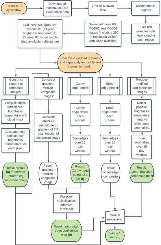
2988                                                                                A. Fraser et al.: Antarctic fast-ice distribution

and continent-wide Antarctic fast-ice dataset from which to          (Fraser et al., 2010), but still involved a significant amount of
accurately gauge change and variability has been highlighted         time-consuming and intensive manual analysis. Considerable
as a major gap by the Intergovernmental Panel on Climate             progress has since been made in the automated extraction of
Change (IPCC) Fifth Assessment Report (Vaughan et al.,               the fast-ice edge in both MODIS (Fraser et al., 2019) and
2013) and the Special Report on the Ocean and Cryosphere             SAR image products (e.g. Kim et al., 2020; Li et al., 2018),
(Meredith et al., 2019).                                             in parallel with advancements in SAR-based fast-ice detec-
   The consistent large-scale and long-term monitoring of            tion in the Arctic, e.g. Mahoney et al. (2007), Meyer et al.
Antarctic fast ice from space necessitates overcoming a num-         (2011), and Dammann et al. (2019). Improved automation is
ber of inherent challenges relating to detection and resolution      particularly important given the volume of data involved and
(both spatial and temporal), given the attributes of the satel-      the considerable effort that is required to manually digitise
lite data themselves, and the nature of fast ice itself. For one     the fast-ice edge using non-automated techniques (Fraser et
thing, fast ice is a narrow remote-sensing target compared to        al., 2012).
the more extensive moving pack ice zone (that is regularly              To date, large-scale and long time-series mapping of
monitored by coarse-resolution satellite passive-microwave           Antarctic fast ice has been confined to two datasets. These
sensors), and advection of pack ice against adjacent fast            are (1) the manually classified MODIS-based dataset (Fraser
ice can lead to a relatively indistinct boundary between the         et al., 2012) and (2) a fully automated time series derived
two. Table 1 summarises the current status of Antarctic fast-        from Advanced Microwave Scanning Radiometer for EOS
ice detection and mapping from space and the advantages              (AMSR-E) for the time period 2003 to 2012 from Nihashi
and disadvantages of the techniques used (see also Lubin             and Ohshima (2015). While the latter dataset is circumpolar
and Massom, 2006). Wide-swath moderate-resolution satel-             in its coverage, an analysis by Fraser et al. (2019) shows a
lite visible and thermal infrared (TIR) imagery offers excel-        tendency of passive-microwave radiometry to underestimate
lent geographical coverage at kilometre-scale resolution and         fast-ice extent due to an inherent insensitivity to young fast
on daily timescales, but it is strongly affected by persistent       ice < 90 d old and its relatively poor spatial resolution.
cloud cover year-round and polar darkness, the latter pre-              Here, we introduce and provide details of a new algorithm
cluding use of visible imagery in winter (Fraser et al., 2009).      and dataset – the first high-spatio-temporal-resolution (1 km;
While this limitation can theoretically be circumvented by           15 d) long-term time series (currently 2000 to 2018 with reg-
using high-resolution synthetic aperture radar (SAR) im-             ular updates planned) of complete circum-Antarctic fast-ice
agery (Giles et al., 2008; Li et al., 2018; Kim et al., 2020), the   extent. This new technique is based on the compositing of
application of SAR to large-scale fast-ice mapping and time-         MODIS cloud-free visible and TIR images using a technique
series analysis has to date been limited in space and time by        described by Fraser et al. (2009) but improved and with au-
its relatively narrow swath coverage and uneven image acqui-         tomated extraction (as far as possible) of the fast-ice edge
sition around coastal Antarctica. Satellite passive-microwave        through addition of edge-detection logic. This reduces the
data, on the other hand, offer complete circumpolar cover-           amount of manual interpretation required while increasing
age on a daily basis (largely unaffected by clouds and dark-         the level of objectivity in retrieving the fast-ice maps.
ness), but a poorer spatial resolution of ∼ 6.25 km (Nihashi            In the next sections, we present a description of the
and Ohshima, 2015) limits its capability for accurate fine-          datasets and updated methods used to transform MODIS
scale mapping of fast ice.                                           imagery into consistent fast-ice maps. Following this, we
   As a result of these challenges and factors relating to sci-      present the fast-ice dataset and provide a comparison with the
entific focus, the mapping of Antarctic fast ice from space          earlier East Antarctic fast-ice time series from Fraser et al.
has to date been largely confined to limited geographical re-        (2012). Analysis of the time series, anomalies, and trends for
gions (e.g. around Antarctic bases and penguin colonies) and         the entire circumpolar record is beyond the scope of this pa-
also relatively short time series or snapshots. These are based      per and is the subject of a study in preparation. A major aim
on manual interpretation of ad hoc digitisations of satellite        here is to make this dataset available to the wider scientific
SAR and cloud-free visible and TIR imagery (e.g. Mae et al.,         community, thereby facilitating collaborative fast-ice-related
1987; Ushio, 2006; Giles et al., 2008; Massom et al., 2009;          research across disciplines.
Aoki, 2017; Kim et al., 2018; Li et al., 2018; Labrousse et al.,
2019; Kim et al., 2020). A significant advance in continuous
coverage was made by Fraser et al. (2012) in their analysis          2   Dataset and methods
of fast ice across East Antarctica (10◦ W to 172◦ E) based
on compositing of cloud-free imagery from the MODerate-              The fast-ice time series presented here for the entire Antarc-
resolution Imaging Spectro-radiometer (MODIS) sensors on             tic coastline uses imagery from the MODIS sensors on both
board NASA’s Aqua and Terra satellites, for the period 2000–         the Terra (MOD) and Aqua (MYD) satellites and obtained
2008. This study also used a more rigorous definition of             from NASA’s Level-1 Atmosphere Archive & Distribution
fast ice that included a temporal criterion, e.g. that sea ice       System Distributed Active Archive Center (https://ladsweb.
must remain stationary for 20 d to be classified as fast ice         modaps.eosdis.nasa.gov, last access: 5 September 2018). The

Earth Syst. Sci. Data, 12, 2987–2999, 2020                                           https://doi.org/10.5194/essd-12-2987-2020
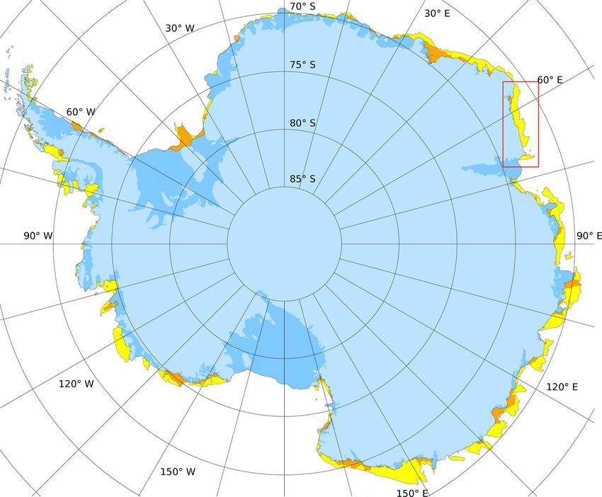
Table 1. Table detailing techniques used to detect and/or map Antarctic fast ice, encompassing both large-scale and case studies. MODIS: Moderate Resolution Imaging Spectrora-
diometer (NASA). AVHRR: Advanced Very High Resolution Radiometer (NOAA). SAR: synthetic aperture radar. SSM/I: Special Sensor Microwave/Imager (Defence Meteorological
Satellite Program). AMSR-E: Advanced Microwave Scanning Radiometer for Earth Observation System (Japan Aerospace Exploration Agency). AMSR2: Advanced Microwave Scan-
ning Radiometer-2 (Japan Aerospace Exploration Agency). ALOS: Advanced Land Observing Satellite (Japan Aerospace Exploration Agency). PALSAR: Phased Array type L-band
Synthetic Aperture Radar (on board ALOS). Envisat: Environment Satellite (European Space Agency). ASAR: Advanced Synthetic Aperture Radar (on board Envisat). RADARSAT:
Radar Satellite (Canadian Space Agency). NA – not available
Product Large-scale dataset Instrument Technique Time span Temporal resolution Spatial resolution Spatial coverage Advantages Disadvantages Publications
https://doi.org/10.5194/essd-12-2987-2020
or case study?
A. Fraser et al.: Antarctic fast-ice distribution
This work Large-scale dataset; MODIS visible– Semi-automated, Mar 2000– 15 d 1 km Circum-Antarctic High spatio-temporal resolution; A degree of subjectivity remains; This work
ongoing thermal IR composite-based Mar 2018; close agreement with Fraser et al. (2012) considerable manual overhead
updates planned long and continuous time series;
semi-automated
MODIS manually Large-scale dataset; MODIS visible– Fully manual, Mar 2000– 20 d 2 km East Antarctica Medium spatio-temporal resolution; Fully manual Fraser et al. (2009, 2010, 2012)
digitised dataset discontinued thermal IR composite-based Dec 2008 continuous time series
Ad hoc MODIS and Case studies MODIS and Fully manual, Nov 1978– Snapshots 1 to 4 km Focus regions Long time series Poor georeferencing and resolution Mae et al. (1987); Massom (2003);
AVHRR digitisations AVHRR visible– snapshots present at times (AVHRR), cloud-affected, Ushio (2006); Massom et al. (2009);
thermal IR fully manual, snapshots Aoki (2017); Kim et al. (2018);
Labrousse et al. (2019)
National Ice Center Large-scale dataset; Various sources Fully manual, Jul 1998– Snapshots within Data- and Circum-Antarctic Long time series; near-real time Unvalidated; fast-ice retrieval of NA
charts ongoing (SAR, visible, snapshots present 1 week year-dependent variable accuracy; not a consistent
TIR, scatterometer) circumpolar format; format changes;
many analysts; fully manual;
coarse spatial resolution at times
Passive microwave Large-scale SSM/I, Principal Dec 1990– 90 d 6.25 to 12.5 km Circum-Antarctic Fully automated Insensitive to young (< 90 d old) fast Tamura et al. (2007, 2016);
spectral dataset; ongoing AMSR-E, component present ice; coarse spatial resolution Nihashi and Ohshima (2015)
AMSR2 analysis
Object-based SAR Case study ALOS Object-based Snapshots in 5d 100 m Various West High spatial resolution; Limited time series of underlying data Kim et al. (2020)
PALSAR definition 2007 and 2010 Antarctic sites reasonable accuracy; potential
for extensive automation
SAR gradient difference Case study Envisat ASAR, Automated ice Snapshots in 13 to 20 d 40 m Prydz Bay High spatial resolution; Requires reference fast-ice climatology Li et al. (2018)
Sentinel 1 edge from 2008 and 2016 high accuracy; potential to remove spurious edges;
gradient difference for extensive automation limited time series of underlying data
Motion-based SAR Case study RADARSAT Maximum Snapshots in 1 to 20 d 100 m Western Pacific High spatial resolution; Limited time series of underlying data Giles et al. (2008)
cross-correlation 1997 and 1999 Ocean sector potential for extensive automation
Multi-sensor fusion Large-scale dataset; MODIS, Machine learning 2003 to 2008 20 d 25 km Circum-Antarctic Novel technique; automated Low spatial resolution; apparent Kim et al. (2015)
discontinued AMSR-E, fast-ice overestimate
SSM/I
Earth Syst. Sci. Data, 12, 2987–2999, 2020
2989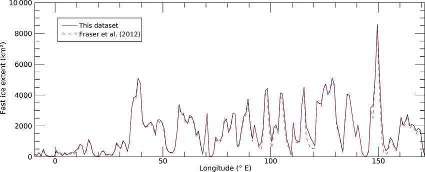
2990                                                                             A. Fraser et al.: Antarctic fast-ice distribution

first ∼ 2 years of this dataset were produced using only Terra    first constructed cloud-free composite images of the surface
MODIS imagery, prior to the July 2002 commissioning of            over consecutive 20 d periods, based on MODIS visible and
Aqua MODIS. Specifically, the algorithm uses data from the        TIR imagery and the NASA MODIS cloud mask product
following:                                                        (Fraser et al., 2009). These composites (i.e. a TIR compos-
                                                                  ite at all times of the year, and a visible composite when
  – channel 1 (visible, 620 to 670 nm) from the
                                                                  solar illumination was present) were then used for manual
    MOD/MYD02QKM dataset, with the 250 m reso-
                                                                  delineation of the fast-ice edge (Fraser et al., 2010). The au-
    lution level 1B product being available during times of
                                                                  thors noted regions and times of lower composite image qual-
    solar illumination;
                                                                  ity when persistent cloud obscured the surface in the major-
  – channel 31 (thermal infrared, 10.78 to 11.28 µm) from         ity of component images (cloud is a major issue for opti-
    MOD/MYD021KM, with the 1 km resolution level 1B               cal remote sensing of the surface in polar regions). In the
    product being available regardless of sunlight and pro-       Fraser et al. (2009) algorithm, even an optically thin layer
    viding information during periods of polar darkness;          of clouds in which the surface features were still discernible
                                                                  was excluded from the cloud-free composite image, some-
  – the high-resolution georeferencing arrays from the            times resulting in “data holes” in the image time series. Here,
    MOD/MYD03 product; and                                        we mitigate this shortcoming by (1) more intelligently rank-
                                                                  ing cloud content and ensuring a more uniform distribution
  – the level 2 cloud mask product (MOD/MYD35_L2).
                                                                  around the Antarctic coast, thereby increasing the chance of
   A crucial feature of the new algorithm and time series is      a cloud-free view of the surface and (2) implementing auto-
accurate masking of the Antarctic continent, ice shelves, and     mated determination of the fast-ice edge location in an in-
nearshore islands. For this, we use the MODIS-based Mosaic        dependent image processing pathway which does not rely
of Antarctica (MOA) coastline digitisation – both the 2003–       on the cloud mask product. Here we rank all cloud mask
2004 product (Haran et al., 2005; Scambos et al., 2007) and       granules by their cloud content, and we choose the 100 least
the 2008–2009 product (Haran et al., 2014). Change in ice         cloudy granules in each of six regions (each approximately
shelf front location over time due to ice sheet advance or ice-   60◦ of longitude wide) around the Antarctic coast for com-
berg calving necessitates progressive updates to the MOA          positing and further processing, i.e. 600 MOD/MYD02 gran-
coastline product. For this, we make annual modifications         ules in total per 15 d window. This regional consideration was
to the location of the ice sheet margin by manually digitis-      implemented in an effort to ensure a more even distribution
ing the change in the position of the ice shelf front once per    of MOD02 granules. We found that without this considera-
year, at the time of annual climatological minimum fast-ice       tion, the ranking algorithm resulted in a high concentration
extent, i.e. days of year 061–075 (Fraser et al., 2012). Tem-     of granules in a limited number of cloud-free regions at the
poral compositing is required to create cloud-free images of      expense of cloudy regions.
the entire Antarctic coastal zone. The MOA-derived annual            In the latter processing pathway described above, we per-
coastline rasters are also manually edited to correct an arte-    form edge detection on all individual gridded MOD/MYD02
fact in the coastline in the Vestfold Hills region, near Davis    granules, exploiting the difference in both albedo and in-
Station (68.5◦ S, 78.25◦ E). Although this process is entirely    frared brightness temperature between ice, cloud, and ocean.
manual, it occurs only once per year so it is not particularly    This is based on the fact that both cloud and pack ice edges
laborious. It is possible that some very persistent multi-year    are dynamic between images whereas fast-ice edges are
fast ice is misclassified as ice shelf in limited regions, al-    likely to be relatively persistent in location (i.e. stationary).
though particular care was paid to avoid this.                    We use the Canny (1986) edge detection method to ensure
   All swath-to-grid projection of the level 1 and 2 im-          that edges are correctly localised and detected only once. We
agery is performed with the MODIS Swath-To-Grid Toolkit           then sum all edges within a 15 d window, thereby determin-
(MS2GT, version 0.26), available at https://nsidc.org/data/       ing which edges are most persistent. These persistent edges
modis/ms2gt (last access: 28 April 2016). We grid all level       are then interpreted to be either the fast-ice edge or the conti-
1 and 2 products to a 1 km resolution polar stereographic         nental margin. Since the location of the continental margin is
grid with a latitude of true scale set to 70◦ S (grid size:       well-known, we exclude these edges from consideration and
5625×4700 pixels, covering the expected maximum circum-           are thus left with a representation of the fast-ice edge. This
polar fast-ice extent), to maximise compatibility with other      map of persistent edges over each 15 d window forms the ba-
sea ice datasets from the NSIDC. We choose a 1 km spatial         sis for subsequent automated circum-Antarctic fast-ice edge
resolution to match the nominal resolution of the MODIS           detection.
TIR channels.                                                        The 15 d time step is chosen by balancing a desire for finer
   We broadly follow the fast-ice mapping methodology de-         resolution against the potential for pack ice temporarily ad-
veloped by Fraser et al. (2009, 2010), but with significant       vected against the coast to be misclassified as fast ice de-
improvements to enhance automation and objectivity in de-         spite no mechanical fastening taking place. Around most of
lineation of the fast-ice edge. The earlier East Antarctic work   coastal Antarctica, the climatological near-surface wind di-

Earth Syst. Sci. Data, 12, 2987–2999, 2020                                        https://doi.org/10.5194/essd-12-2987-2020
A. Fraser et al.: Antarctic fast-ice distribution 2991
rection is generally offshoreward to westward (Turner and sum within the current 15 d period, with the out-
Pendlebury, 2004), thus promoting advection of pack ice come of a canny edge sum image for automated
away from the coast. Blocking anticyclonic pressure sys- edge extraction.
tems do occur in southern mid-latitudes and these can result – Produce Sobel edge images for each granule (So-
in persistent onshoreward winds in particular regions of the bel, 2014). Sobel edge-detect MOD/MYD02 gran-
Antarctic coast, although the residence time for such systems ules and sum within the current 15 d period, with
is rarely longer than 1 week (Massom et al., 2004). As such, the outcome of a Sobel edge sum image to guide
a time step of 15 d is sufficiently long to preclude most of manual fast-ice edge interpretation.
these cases. Drifting sea ice pinned between grounded ice-
bergs may also be misclassified as fast ice, though our earlier – Produce images of the gradient of the median com-
work showed that the persistent advection of pack ice into posite. Median-filter (using a 7 px × 7 px sliding
pre-existing coastal features is likely to be a larger problem window) each composite image (i.e. visible and
and that pack ice held fast between grounded icebergs may TIR), and then take the absolute value of the gra-
quickly become fastened (Fraser et al., 2010). Cloud cov- dient of this image, indicating edges in the com-
erage, which can be persistent in some regions, is a further posite image, with the outcome being images of the
barrier to a finer time step when producing visible and TIR gradient of the mean composite for automated edge
composite images of the surface (Fraser et al., 2009). extraction.
Our image processing pipeline is outlined below and is de- – Produce modified lead-detection images after
picted by a flow chart in Fig. 1. For each 15 d window in the Willmes and Heinemann (2015). We use a larger fil-
March 2000 to March 2018 study period, we do the follow- tering window of 251 pixels (originally 51 pixels)
ing. to enhance contrast in regions of fast ice, with the
outcome of lead-detection images to guide manual
1. We download and grid all MOD/MYD35_L2 (cloud fast-ice edge interpretation.
mask) granules covering the Antarctic coastal zone (ap-
proximately 1800 granules per 15 d interval), with the 6. Construct an automated classification base image.
outcome of a complete library of gridded cloud mask
– Compute the per-pixel product of the Canny edge
granules.
image and the gradient-median-composite image
2. We rank granules by cloud content, with the outcome of described above, which was found to accurately and
a ranked list of least-cloudy scenes. correctly locate many fast-ice edges (i.e. this is an
original algorithm). This product represents a con-
3. We select the top 600 cloud-free granules, cognisant tinuous measure of fast-ice edge confidence. This
of granule location (to ensure sufficient coverage in all results in a base image for automated fast-ice edge
coastal regions), with the outcome of a list of 600 least- extraction.
cloudy scenes with relatively even coverage around the
continent. – Produce a normalised histogram of edge confi-
dence, setting four adaptive thresholds at 0.995
4. We download and grid all corresponding (highest-confidence edge), 0.990, 0.985, and 0.980
MOD/MYD02QKM (reflectance, available during (lowest-confidence edge). These thresholds are
periods of solar illumination), MOD/MYD021KM used to construct a greyscale representation of the
(TIR brightness temperature, available year-round), edge confidence for each pixel on the grid. This re-
and MOD/MYD03 (high-resolution geolocation data) sults in a confidence-classified automated fast-ice
granules, with the outcome of a library of least-cloudy edge map.
reflectance and TIR brightness temperature scenes, – Mask the edge confidence map using the rasterised
gridded. MOA coastline and write out as the automated clas-
5. We process gridded MOD/MYD02 images for manual sification base image. Multiple spurious edges exist
and automated edge-detection purposes. at this point. This results in a coast-masked auto-
mated edge image.
– Produce cloud-free composite images from 600 in-
put granules. Construct thermal infrared and (when 7. Carry out necessary manual processing (relatively
solar illumination available) visible cloud-free labour-intensive; 1 year takes approximately 40 h).
composite images from the gridded MOD/MYD02 – Closely inspect and complete edges in automated
and MOD/MYD35_L2 granules, following Fraser classification base image, guided by (a) the So-
et al. (2009, 2010), with the outcome cloud-free. bel edge image, (b) cloud-free composites, and
– Produce Canny edge images for each granule. (c) modified lead-detection images. This is used
Canny edge-detect MOD/MYD02 granules and to (i) verify automated fast-ice edge extraction and
https://doi.org/10.5194/essd-12-2987-2020 Earth Syst. Sci. Data, 12, 2987–2999, 20202992 A. Fraser et al.: Antarctic fast-ice distribution
(ii) manually complete/add edges where automated the manual digitisation error by carrying out an independent
extraction fails to detect the fast-ice edge. Sobel re-digitisation of a subset of the fast-ice edge and resolving
edge detection is used in this manual step rather differences in the resulting fast-ice area (Fraser et al., 2010).
than Canny edge detection, because it produces a This approach, however, requires both extrapolation of er-
broader (i.e. several pixels wide) edge which is tol- rors from a small subset to the entire dataset and duplica-
erant of small changes in ice edge location. This tion of time-consuming manual edge extraction. In our mod-
results in an image of completed fast-ice edges. ified approach presented here, we employ a novel alternative
– “Bucket-fill” those pixels between the continental approach for uncertainty estimation which addresses these
margin and the now-continuous ice edge to rep- shortcomings. This involves analysis of the per-pixel differ-
resent fast-ice coverage (extent). This results in a ence in ice edge location in two consecutive fast-ice maps,
near-final image of fast-ice edge and “filled” pix- for all pairs of consecutive images in the entire dataset. In
els. the case of an automatically extracted fast-ice edge pixel,
this difference purely reflects the change in location of the
8. Automatically remove spurious edges (i.e. edges not ad- ice edge (plus or minus a small, sub-pixel-scale digitisation
jacent to fast ice) remaining from the classified image. error, which we also quantify). In the case of a manually
This results in a final classified fast-ice image. extracted ice edge pixel, it reflects the sum of the ice edge
change plus the digitisation error. Thus, to estimate the digi-
Since the bucket-fill step requires a continuous fast-ice tisation uncertainty, we do the following.
edge, and because the automatically determined fast-ice edge
1. Assume that automatically determined edges are accu-
is often incomplete, manual intervention is frequently re-
rate in location (an appropriate assumption due to excel-
quired both to form a continuous fast-ice edge and to val-
lent edge localisation of the Canny edge detection filter
idate the position of the automatically determined fast-ice
underpinning the automation).
edge. An example classification showing both manual and
automated ice edge detection is shown in Fig. 2. This manual 2. Quantify the mean fast-ice edge separation between
intervention is relatively time-consuming and reduces objec- subsequent images only for automatically determined
tivity to some extent but is considered to be a fundamental edge pixels. We find the nearest edge of similar type.
step in visible–TIR fast-ice extent retrieval. It should be re- In this step, we match automatically determined edge
iterated here that the inclusion of automatic edge determina- pixels with the nearest automatically determined edge
tion is a considerable advance from the original fully man- in the subsequent image. Cross-type edge matches are
ual final step of edge extraction described by Fraser et al. ignored (i.e. auto to manual or manual to auto) to
(2010). In order to mitigate the possibility of manual edge avoid confounding results. A cutoff of ±50 px (i.e. an
definition contributing to false trends in the dataset and fol- ∼ 100 km window) is used as an extremely conservative
lowing Fraser et al. (2012), all edge verification and manual upper bound to avoid the rare case of pixels matching
edge completion is performed in a random order. with distant pixels. We thereby produce a mean mea-
When manual edge delineation is not possible in any given sure of ice edge location change between two consecu-
region for a particular 15 d period (e.g. due to persistent thick tive 15 d time periods.
cloud), the method employs a subjective definition of the lo-
cation of the fast-ice edge based on imagery from the im- 3. Carry out the same as above but for manually deter-
mediately previous and/or subsequent 15 d periods, follow- mined edge pixels, to produce a mean measure of ice
ing Fraser et al. (2010). An extreme example relates to the edge change plus digitisation error.
fast-ice map from DOYs 166–180 in 2001, during most of
4. Subtract the former from the latter, resulting in a digiti-
which the Terra MODIS instrument was in “safe mode” and
sation error estimate for manually determined ice edge
acquired no data. Here, in the interest of providing a tempo-
pixels.
rally contiguous dataset, we opt to use the fast-ice map from
the following time step (DOYs 181–195, 2001) but mark all We also estimate the sub-pixel error in digitisation, i.e.
edges as “manually determined” to indicate higher uncer- grid-scale effects in the digitisation error. This estimation
tainty in the fast-ice edge retrieval for DOYs 181–195 (2001). is achieved by performing 10 000 simulations of a one-
Determination of uncertainty for this dataset (in both edge dimensional random edge position and compare it to the cen-
location and resulting fast-ice areal extent) requires careful tre location of a sample pixel. The rms of the residual be-
consideration. The primary uncertainty arises from digitisa- tween the genuine pixel centre and the simulated centre is
tion error, typically given in pixels, in areas of manual ice taken to be the sub-pixel error. Thus, the automatically deter-
edge determination, which then propagates to an areal un- mined edge error is taken to be the sub-pixel error only, and
certainty value. However, neither the digitisation error nor the manually determined edge error is taken to be the quadra-
the propagation to an areal uncertainty is straightforward to ture sum of the sub-pixel and manual digitisation errors. Fol-
determine and quantify. Prior work made broad estimates of lowing estimation of both the manual and sub-pixel digiti-
Earth Syst. Sci. Data, 12, 2987–2999, 2020 https://doi.org/10.5194/essd-12-2987-2020A. Fraser et al.: Antarctic fast-ice distribution 2993
Figure 1. Flow chart depicting the image processing pipeline. Bold letters within the green-coloured elements refer to individual panels in
Fig. 2.
sation errors, we estimate areal uncertainty for each fast-ice 2. weighting all skeletonised edge pixels by their respec-
map by tive area, and then
1. ensuring that all fast-ice edges are 1 pixel wide by per- 3. multiplying by the appropriate error, as estimated
forming a morphological skeleton operation, above.
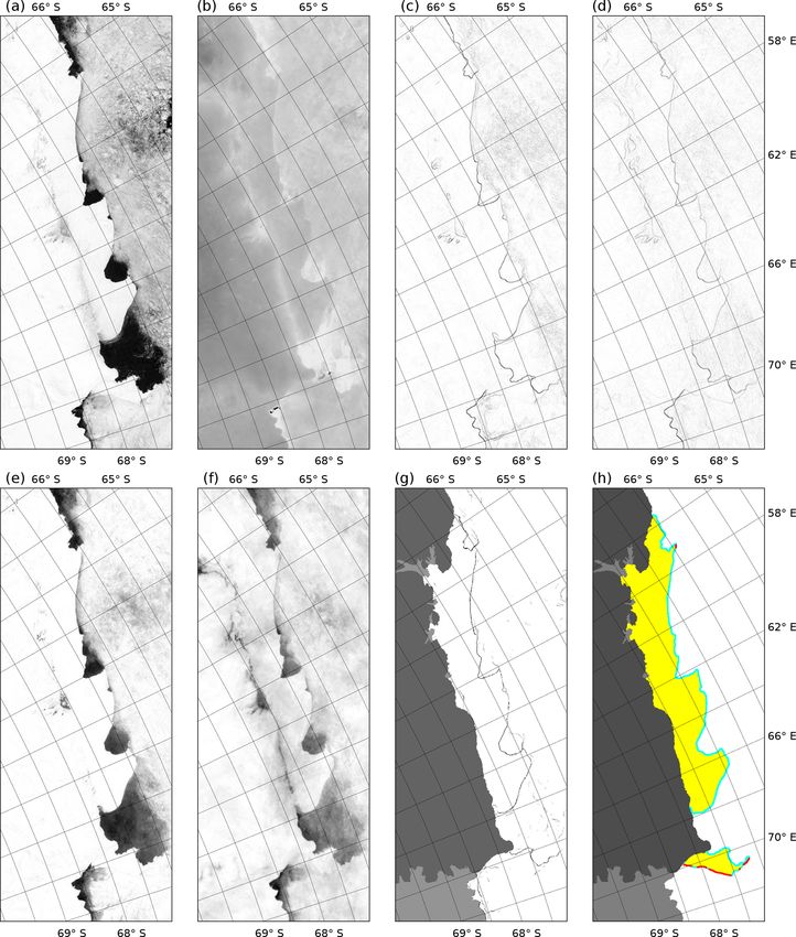
https://doi.org/10.5194/essd-12-2987-2020 Earth Syst. Sci. Data, 12, 2987–2999, 20202994 A. Fraser et al.: Antarctic fast-ice distribution Figure 2. Figure depicting an example of the automated fast-ice edge detection along the Mawson Coast, East Antarctica, for DOY range 316–330, 2005. See the red rectangle in Fig. 3 for spatial context. (a, b) The 15 d channel 1 (visible) and channel 31 (thermal infrared) cloud-free composite images, respectively. (c, d) Sum of Canny algorithm-detected edges in individual channel 1 and channel 31 images, respectively, for the 15 d period. (e, f) Modified lead detection for channel 1 and channel 31 images, respectively (after Willmes and Heine- mann, 2015, but with an enlarged filtering window to enhance fast-ice detection). (g) Results of the combined edge detection algorithm (black line). Light and dark grey areas represent grounded and floating glacial ice, respectively, and are masked out. (h) Fast-ice classified map after manual edge inspection/correction and filling. Cyan and red represent automatically and manually completed edges, respectively, and the width of these lines has been expanded in this example to enhance visibility. Yellow represents infilled fast-ice area. Earth Syst. Sci. Data, 12, 2987–2999, 2020 https://doi.org/10.5194/essd-12-2987-2020
A. Fraser et al.: Antarctic fast-ice distribution                                                                              2995

   This approach to areal uncertainty calculation is highly
conservative (i.e. likely an overestimate) since it assumes that
all errors occur in the same direction; in reality, digitisation
errors are likely to produce both underestimates and overes-
timates of fast-ice extent in equal measure. Furthermore, cy-
clonic systems which may cause windblown regional fast-ice
breakout (Massom et al., 2009) also typically bring extensive
cloud cover. In this way, image subsets requiring manual fast-
ice edge delineation are more likely to be produced during
times of wholesale ice edge change, thereby falsely inflating
the uncertainty estimates.
   Regarding the fast-ice dataset product, we provide the
method of edge determination (“automatic” or “manual”) in
the output dataset, for each pixel of fast-ice edge. We also
compute the mean percentage of automatically determined
ice edge pixels in each 1◦ longitude bin. As a further indi-
cation of dataset integrity, we quantify differences between
the new fast-ice dataset and the Fraser et al. (2012) East
                                                                    Figure 3. Fast-ice distribution at times of maximum (occurring
Antarctic-only dataset for the period and region of overlap
                                                                    in 2006, DOYs 271–285; shown in yellow) and minimum (2009,
(north of 72◦ S, 10◦ W to 172◦ E, March 2000 to Decem-
                                                                    DOYs 061–075; shown in orange) extent over the 18-year dataset
ber 2008). Large tabular icebergs are removed from the fast-        period. The grounded Antarctic Ice Sheet and floating ice shelves
ice classification where independent iceberg information is         are shaded light and dark blue, respectively. The red rectangle
available and/or the icebergs are clearly visible, but manual       shows the region used to illustrate the automation in Fig. 2.
discrimination between fast ice and large tabular icebergs is
difficult at times due to a lack of contrast in the satellite im-
agery (Fraser et al., 2010). Similarly, myriads of small ice-
bergs embedded/grounded in places in the fast ice (Massom           dataset with that of Fraser et al. (2012), covering the area and
et al., 2009) are difficult to distinguish and remove, but they     period of overlap. The total East Antarctic fast-ice extent in
form an integral part of the fast-ice matrix. Following Fraser      the new dataset is 8.3 % greater than that reported in Fraser
et al. (2010), we classify such regions of fast ice contain-        et al. (2012), on average. This difference is attributed to two
ing many small grounded icebergs as fast ice. Regions of ice        factors: (1) a “relaxation” of the temporal fast-ice condition
mélange at the front of ice shelves are another source of un-       in the new algorithm from the 20 d criterion used in Fraser
certainty here, but they remain unquantified due to their neg-      et al. (2012) (i.e. more ice remains “fast” for 15 d than for
ligible areal extent on a continental scale.                        20 d) and (2) the enhanced ability of the new “persistence
                                                                    of edges” algorithm to retrieve fast-ice extent under cloud
3     Results and brief discussion                                  cover. The largest differences between the two datasets are
                                                                    encountered at ∼ 118 and 152◦ E. These two longitudes cor-
We restrict our presentation of results to illustration of the      respond to areas of dynamically formed “semi-fast ice”, i.e.
key attributes of this new pan-Antarctic fast-ice dataset, and      regions where pack ice is blocked from westward advection
we evaluate its improvements over earlier datasets created for      and intercepted by upstream obstacles, e.g. large grounded
East Antarctica (Fraser et al., 2012). We also present quan-        iceberg B9B prior to its ungrounding in 2010 (Massom et al.,
tification of uncertainties. More in-depth analysis of spatio-      2010). In such regions, fast ice tends to be more exposed and
temporal patterns and drivers of fast-ice distribution is out-      ephemeral; i.e. it can intermittently break out to become pack
side the scope of this paper but is underway for future stud-       ice but then reform, on a synoptic scale. As such, reducing
ies.                                                                the temporal “fastness” condition to 15 d produces relatively
                                                                    large differences in these regions.
                                                                       This sensitivity of fast-ice extent to observation time step
3.1    Circumpolar distribution of fast ice at maximum and
                                                                    has implications not only for the current work, but also for
       minimum extent and cross-comparison with earlier
                                                                    the next generation of SAR-based observations of fast ice,
       work
                                                                    which, depending on the algorithm, can rely on two obser-
We illustrate the envelope of circum-Antarctic fast-ice ex-         vations obtained in subsequent repeat passes. In the case of
tent throughout the 18-year dataset time series by showing          the ESA’s Sentinel-1, this involves a 12 d repeat cycle. The
its spatial distribution at maximum (occurring in 2006, at          temporal baseline of DLR’s TerraSAR-X is shorter still at
DOYs 271–285) and minimum (2009, DOYs 061–075) ex-                  11 d, although it has yet to be exploited for fast-ice retrieval.
tent in Fig. 3. Figure 4 then shows a cross-comparison of this      Other SAR-based fast-ice retrieval algorithms which do not

https://doi.org/10.5194/essd-12-2987-2020                                          Earth Syst. Sci. Data, 12, 2987–2999, 2020
2996 A. Fraser et al.: Antarctic fast-ice distribution
Figure 4. Mean fast-ice extent per degree of longitude for this new improved dataset (black solid line) and Fraser et al. (2012) (dashed red
line), for the period and region of time series overlap (March 2000 to December 2008, 10◦ W to 172◦ E).
rely on exact repeat orbits are able to retrieve fast-ice extent and George V lands (150 to 153◦ E). In West Antarctica, au-
over even shorter baselines (e.g. feature-tracking algorithms tomation percentage is high (generally 70 % to 90 %) in the
can deal with any baseline, as long as features are present). eastern Weddell Sea and Ross Sea (50 % to 85 %) but low in
Such methods are all likely to retrieve higher fast ice ex- the Bellingshausen and Amundsen seas sector (40 % to 60 %)
tents than the product here, simply due to the shorter obser- and along both flanks of the Antarctic Peninsula (as low as
vational baseline. As indicated here, differences are particu- 22 %). By showing longitudes with a low automation frac-
larly strong in regions containing volatile fast ice. As such, tion, this plot also indicates areas which tend to be most af-
end-users of fast-ice products in such regions should be cog- fected by inherent issues detailed in the Methods section, i.e.
nisant of this phenomenon. persistent cloud cover and/or persistent advection of pack ice
toward fast ice that reduces the contrast (in reflectance and
3.2 Quantification of dataset objectivity and error surface temperature) between pack and fast ice.
estimation We have taken steps to mitigate this here compared to
our earlier work (e.g. by now considering edges visible even
Both the cloud-free composite images and the automated under thin cloud, by more intelligently selecting the least-
classification base images are susceptible to a number of fac- cloudy MODIS data for each 15 d period). Here, our ap-
tors which can reduce their quality/utility as fast-ice edge dis- proach is still limited by relatively poor MOD/MYD35 cloud
criminators. These include (1) persistent/heavy cloud obscu- mask product accuracy at times. In the future, we are in-
ration of the surface – particularly during times of no solar terested in implementing state-of-the-art machine-learning
illumination when the cloud mask product is less accurate cloud masking algorithms to mitigate this (e.g. Paul and
(Ackerman et al., 2006) and (2) instances where moving pack Huntemann, 2020). This improvement may lead to an au-
ice is advected toward the fast-ice edge, thereby reducing the tomation percentage in excess of the 58 % reported here.
fast-ice–pack ice contrast in both visible and TIR images, as As detailed in the Methods section, we estimated the sub-
noted in Fraser et al. (2009). pixel error, applicable to both automatically and manually
Manual delineation ranges from being relatively straight- determined edges, as well as the manual-only error in digi-
forward (in the case of high-quality composite imagery, tisation. By simulation, the sub-pixel error is determined to
where few judgement calls need to be made) to quite labour be 0.288 pixels. We developed a novel technique to quantify
intensive (in the case of heavy cloud obscuring the surface, the error in manual estimation of fast-ice edges. We find that,
resulting in ambiguous fast-ice edge delineation and requir- on average, manually determined edges change in location
ing the use of the previous and next 15 d period’s composite by 5.47 pixels more than that for automatically determined
imagery for guidance). On occasion, such judgement calls edges (auto-determined = 10.06 pixels vs. manually deter-
have the potential to significantly impact a single period’s mined = 15.53 pixels) in subsequent 15 d windows. Thus,
fast-ice extent retrieval, albeit in a limited region. the automatically determined edge error is 0.288 pixels, and
A broad measure of objectivity in fast-ice extent retrieval the manually determined edge error is the quadrature sum
is the percentage of edges that could be retrieved automati- of 0.288 and 5.47 pixels, i.e. 5.48 px. For each 15 d epoch,
cally. This is plotted in Fig. 5. The circum-Antarctic mean we obtain a conservative estimate of the fast-ice areal un-
automation percentage is 58 %. East Antarctica is charac- certainty by multiplying each skeletonised edge pixel by the
terised by generally high automation percentages (∼ 50 % appropriate error estimate, in kilometres, assuming that the
to 90 %) – with the exception of localised pockets (down to nominal resolution of 1 km per pixel applies everywhere in
37 %) located in Wilkes (98 to 108◦ E and 126 to 138◦ E)
Earth Syst. Sci. Data, 12, 2987–2999, 2020 https://doi.org/10.5194/essd-12-2987-2020A. Fraser et al.: Antarctic fast-ice distribution 2997
5 Summary
Here we have introduced both (1) a new, improved technique
for mapping and monitoring coastal fast-ice coverage around
Antarctica at high resolution and (2) the most complete time
series of Antarctic fast-ice extent to date. This product repre-
sents a new baseline against which to gauge change and vari-
ability in both the ice and climate and has wide applicability.
Indeed, it is expected to generate and contribute to multi-
ple cross-disciplinary studies of the Antarctic coastal envi-
ronment. Examples include behavioural ecology of charis-
matic megafauna (e.g. emperor penguin colony presence or
absence), the effects of fast ice on the physical oceanogra-
phy of the continental shelf (e.g. influencing coastal polynya
location, and subsequent sea ice production and water mass
modification), and a quantification of the fresh water, nutri-
ents, and biomass within the fast ice itself. Logistical uses
are also envisioned (e.g. informing base resupply schedules).
Moreover, this dataset directly addresses a key gap identified
in major high-level IPCC reports, enabling improved analysis
of trends and variability of this key element of the highly vul-
nerable Antarctic coastal environment (Vaughan et al., 2013;
Figure 5. Polar plot showing the percentage of edges determined Meredith et al., 2019).
automatically, as a function of longitude. The Antarctic continent is The new algorithm also provides an important means of
outlined in grey for spatial context. To remove noise in regions with mapping and monitoring fast ice into the future and in a
little fast ice, 1◦ longitude bins with fewer than 5000 total fast-ice continuous fashion, given its applicability to the new gen-
edge pixels across the 18-year dataset were not plotted. eration of medium-resolution spectroradiometers. These in-
clude the Visible Infrared Imaging Radiometer Suite (VI-
IRS) on NASA’s Suomi National Polar-orbiting Partnership
the domain. This uncertainty in fast-ice area has a mean value (NPP) platform (launched October 2011), the Sea and Land
of 7.8 % when averaged across the entire circum-Antarctic Surface Temperature Radiometer (SLSTR) and Ocean and
dataset. This is somewhat larger the value of 4.38 % uncer- Land Colour Instrument (OLCI) on ESA’s Sentinel-3 plat-
tainty obtained in regions requiring > 10 % manual edge de- form (launched February 2016), and the Second-generation
lineation, as detailed in Fig. 5 from Fraser et al. (2010) using Global Imager (SGLI) on JAXA’s Global Change Obser-
traditional re-digitisation-based error estimation, confirming vation Mission (GCOM)-C1 platform (launched December
that the new method is conservative. 2017).
Although an element of subjectivity remains in the large-
4 Data availability scale retrieval of fast-ice coverage from satellite visible–
thermal infrared imagery, we have mitigated this to some
The dataset has been made available at the Australian Antarc- extent. This has been achieved by (1) implementing an au-
tic Data Centre at https://doi.org/10.26179/5d267d1ceb60c, tomated ice edge retrieval algorithm, resulting in successful
as a series of NetCDF files compliant with Climate and Fore- extraction of ∼ 58 % of ice edge pixels; (2) performing ran-
cast (CF) (Fraser et al., 2020). This dataset contains the fol- dom manual extraction to eliminate false trends; (3) quantify-
lowing fields: ing the uncertainty associated with manual edge delineation
(7.8 % of fast-ice area retrieval, on average); and (4) per-
– fast-ice time series – presented as classified maps of the forming a cross-comparison with a similar (but independent)
surface type (fast-ice interior pixel, automatically deter- spatially and temporally overlapping dataset (Fraser et al.,
mined fast-ice edge, manually determined fast-ice edge) 2012). Crucially, this new MODIS-based dataset provides
– and the longest contiguous time series of this key element of
– latitude, longitude, and area of each pixel. the Antarctic cryosphere while offering complete circum-
Antarctic coverage for the first time at high resolution.
There are plans to regularly update and extend the time se- Multi-sensor fusion would help to further mitigate the sub-
ries forwards in time, on a biennial basis, until the demise of jective elements of this dataset to some extent. As an exam-
both MODIS platforms but continuing with next-generation ple, we used AMSR-E, in our previous work (Fraser et al.,
imaging spectroradiometers after this time. 2010). However, mission overlap generally limits the time
https://doi.org/10.5194/essd-12-2987-2020 Earth Syst. Sci. Data, 12, 2987–2999, 20202998 A. Fraser et al.: Antarctic fast-ice distribution
period able to be considered in multi-sensor fusion algo- no. NE/L002531/1), and the Australian Research Council (grant no.
rithms (e.g. AMSR-E was launched 2.5 years after Terra SR140300001).
MODIS and was effectively decommissioned in 2011).
Analysis of spatio-temporal patterns, variability, and
trends in circum-Antarctic fast-ice coverage is underway, us- Review statement. This paper was edited by Ge Peng and re-
ing this dataset (Fraser et al., 2020), as is related work deter- viewed by four anonymous referees.
mining and evaluating the drivers of these observed patterns.
Moreover, we plan to study the spatial distribution of fast-ice
extent in the context of a new dataset describing the multi- References
scale complexity and configuration of the coastline (includ-
ing aspect) around Antarctica (Porter-Smith et al., in review, Ackerman, S. A., Strabala, K. I., Menzel, W. P., Frey, R. A., Moeller,
2019), under the hypothesis that the coastal configuration is C. C., Gumley, L. E., Baum, B., Seemann, S. W., and Zhang, H.:
a first-order determinant of fast-ice extent in many regions. Discriminating clear-sky from cloud with MODIS, Algorithm
Theoretical Basis Document ATBD-MOD-06, NASA Goddard
Space Flight Center, Greenbelt, Maryland, 2006.
Author contributions. ADF led the study, acquired the data, de- Aoki, S.: Breakup of landfast sea ice in Lützow-Holm Bay, East
veloped automation algorithms, manually digitised fast ice, pro- Antarctica, and its teleconnection to tropical Pacific sea surface
duced figures, and wrote the manuscript. RAM and KIO contributed temperatures, Geophys. Res. Let., 44, 3219–3227, 2017.
equally toward project genesis and direction. SW contributed to al- Canny, J.: A Computational Approach to Edge Detection, IEEE T.
gorithm automation development. PJK assisted with manual digiti- Pattern Anal., 6, 679–698, 1986.
sation. JC and RPS packaged the dataset for distribution. All authors Dammann, D. O., Eriksson, L. E. B., Mahoney, A. R., Eicken, H.,
edited the manuscript. and Meyer, F. J.: Mapping pan-Arctic landfast sea ice stability
using Sentinel-1 interferometry, The Cryosphere, 13, 557–577,
https://doi.org/10.5194/tc-13-557-2019, 2019.
Fraser, A. D., Massom, R. A., and Michael, K. J.: A
Competing interests. The authors declare that they have no con-
Method for Compositing Polar MODIS Satellite Im-
flict of interest.
ages to Remove Cloud Cover for Landfast Sea-Ice De-
tection, IEEE T. Geosci. Remote S., 47, 3272–3282,
https://doi.org/10.1109/TGRS.2009.2019726, 2009.
Acknowledgements. MODIS data were obtained from the Fraser, A. D., Massom, R. A., and Michael, K. J.: Generation of
NASA Level-1 Atmosphere Archive & Distribution System Dis- high-resolution East Antarctic landfast sea-ice maps from cloud-
tributed Active Archive Center at https://ladsweb.modaps.eosdis. free MODIS satellite composite imagery, Remote Sens. Envi-
nasa.gov (last access: 5 September 2018). This work was supported ron., 114, 2888–2896, https://doi.org/10.1016/j.rse.2010.07.006,
by the Australian Government’s Cooperative Research Centre pro- 2010.
gramme through the Antarctic Climate & Ecosystems Coopera- Fraser, A. D., Massom, R. A., Michael, K. J., Galton-Fenzi,
tive Research Centre; the Japan Society for the Promotion of Sci- B. K., and Lieser, J. L.: East Antarctic Landfast Sea Ice Dis-
ence Grant-in-Aid for Scientific Research (KAKENHI) numbers tribution and Variability, 2000-08, J. Climate, 25, 1137–1156,
25·03748, 24·810030, 25·241001, 26·740007, and 17H01157; by https://doi.org/10.1175/JCLI-D-10-05032.1, 2012.
the Canon Foundation; the Natural Environment Research Council Fraser, A. D., Ohshima, K. I., Nihashi, S., Massom, R. A., Tamura,
(grant NE/L002531/1); and the Australian Research Council’s Spe- T., Nakata, K., Williams, G. D., Carpentier, S., and Willmes, S.:
cial Research Initiative for Antarctic Gateway Partnership (project Landfast ice controls on sea-ice production in the Cape Darn-
ID SR140300001). This work also contributes to Australian Antarc- ley Polynya: A case study, Remote Sens. Environ., 233, 111315,
tic Science Project 4116, the Australian Antarctic Program Part- https://doi.org/10.1016/j.rse.2019.111315, 2019.
nership and the World Climate Research Programme (WCRP) Cli- Fraser, A. D., Massom, R. A., Ohshima, K. I., Willmes, S., Kappes,
mate and Cryosphere (CliC) Project initiative Interactions Between P., Cartwright, J., and Porter-Smith, R.: Circum-Antarctic land-
Cryospheric Elements. Robert A. Massom acknowledges the sup- fast sea-ice extent, 2000-2018, Australian Antarctic Data Centre,
port of the Australian Antarctic Division. Alexander D. Fraser is https://doi.org/10.26179/5d267d1ceb60c, 2020.
grateful to David Fanning for maintaining the Coyote library of IDL Giles, A. B., Massom, R. A., and Lytle, V. I.: Fast-ice distribu-
routines, many of which were used in this work, to Terry Haran tion in East Antarctica during 1997 and 1999 determined us-
(NSIDC) for developing the MODIS Swath-To-Grid Toolbox, and ing RADARSAT data, J. Geophys. Res.-Oceans, 113, C02S14,
to Chad Greene for discussions around the distribution of the data. https://doi.org/10.1029/2007JC004139, 2008.
Haran, T. M., Bohlander, J., Scambos, T. A. Painter, T.,
and Fahnestock, M. A.: MODIS Mosaic of Antarc-
Financial support. This research has been supported by the Aus- tica 2003–2004 (MOA2004) image map, Digital media,
tralian Government (grant Antarctic Climate & Ecosystems Coop- https://doi.org/10.7265/N5ZK5DM5, 2005.
erative Research Centre), the Japan Society for the Promotion of Haran, T. M., Bohlander, J., Scambos, T. A., Painter, T.,
Science (grant nos. 25·03748, 24·810030, 25·241001, 26·740007, and Fahnestock, M. A.: MODIS Mosaic of Antarc-
and 17H01157), the Natural Environment Research Council (grant tica 2008–2009 (MOA2009) image map, Digital media,
https://doi.org/10.7265/N5KP8037, 2014.
Earth Syst. Sci. Data, 12, 2987–2999, 2020 https://doi.org/10.5194/essd-12-2987-2020A. Fraser et al.: Antarctic fast-ice distribution 2999 Kim, M., Im, J., Han, H., Kim, J., Lee, S., Shin, M., and Kim, H.- Meyer, F. J., Mahoney, A., Eicken, H., Denny, C. L., Druck- C.: Landfast sea ice monitoring using multisensor fusion in the enmiller, H. C., and Hendricks, S.: Mapping Arctic land- Antarctic, GIScience & Remote Sens., 52, 239–256, 2015. fast ice extent using L-band synthetic aperture radar Kim, M., Han, H., Im, J., Lee, S., and Kim, H.-C.: Object-based interferometry, Remote Sens. Environ., 115, 3029–3043, Landfast Sea Ice Detection Over West Antarctica Using Time https://doi.org/10.1016/j.rse.2011.06.006, 2011. Series of ALOS PALSAR Data, Remote Sens. Environ., 242, Nihashi, S. and Ohshima, K. I.: Circumpolar mapping of Antarctic 111782, https://doi.org/10.1016/j.rse.2020.111782, 2020. coastal polynyas and landfast sea ice: Relationship and variabil- Kim, S., Saenz, B., Scanniello, J., Daly, K., and Ain- ity, J. Climate, 28, 3650–3670, 2015. ley, D.: Local climatology of fast ice in McMurdo Paul, S. and Huntemann, M.: Improved machine-learning based Sound, Antarctica, Antarctic Science, 30, 125–142, open-water/sea-ice/cloud discrimination over wintertime Antarc- https://doi.org/10.1017/S0954102017000578, 2018. tic sea ice using MODIS thermal-infrared imagery, The Labrousse, S., Fraser, A. D., Sumner, M., Tamura, T., Pinaud, D., Cryosphere Discuss., https://doi.org/10.5194/tc-2020-159, in re- Wienecke, B., Kirkwood, R., Ropert-Coudert, Y., Reisinger, R., view, 2020. Jonsen, I., Porter-Smith, R., Barbraud, C., Bost, C.-A., Ji, R., and Porter-Smith, R., McKinlay, J., Fraser, A., and Massom, R.: Coastal Jenouvrier, S.: Dynamic fine-scale sea-icescape shapes adult em- complexity of the Antarctic continent, Earth Syst. Sci. Data Dis- peror penguin foraging habitat in East Antarctica, Geophys. Res. cuss., https://doi.org/10.5194/essd-2019-142, in review, 2019. Lett., 46, 11206–11218, 2019. Scambos, T., Haran, T., Fahnestock, M., Painter, T., and Boh- Li, X., Ouyang, L., Hui, F., Cheng, X., Shokr, M., and Heil, P.: An lander, J.: MODIS-based Mosaic of Antarctica (MOA) data sets: Improved Automated Method to Detect Landfast Ice Edge off Continent-wide surface morphology and snow grain size, Re- Zhongshan Station Using SAR Imagery, IEEE J. Sel. Top. Appl., mote Sens. Environ., 111, 242–257, 2007. 11, 4737–4746, https://doi.org/10.1109/JSTARS.2018.2882602, Sobel, I.: An Isotropic 3x3 Image Gradient Operator, Presentation 2018. at Stanford A.I. Project 1968, 2014. Lubin, D. and Massom, R. A.: Polar Remote Sensing Volume I: At- Tamura, T., Ohshima, K. I., Markus, T., Cavalieri, D. J., Ni- mosphere and Oceans, Praxis/Springer, Chichester/Berlin, 2006. hashi, S., and Hirasawa, N.: Estimation of Thin Ice Thick- Mae, S., Yamanouchi, T., and Fujii, Y.: Remote sensing of fast ice ness and Detection of Fast Ice from SSM/I Data in the in Lützowholmbukta, East Antarctica, using satellite NOAA-7, 8 Antarctic Ocean, J. Atmos. Ocean. Tech., 24, 1757–1772, and aircraft, Ann. Glaciol., 9, 251–251, 1987. https://doi.org/10.1175/JTECH2113.1, 2007. Mahoney, A., Eicken, H., Gaylord, A. G., and Shapiro, L.: Tamura, T., Ohshima, K. I., Fraser, A. D., and Williams, Alaska landfast sea ice: Links with bathymetry and atmo- G. D.: Sea ice production variability in Antarctic coastal spheric circulation, J. Geophys. Res.-Oceans, 112, C02001, polynyas, J. Geophys. Res.-Oceans, 121, 2967–2979, https://doi.org/10.1029/2006JC003559, 2007. https://doi.org/10.1002/2015JC011537, 2016. Massom, R. A.: Recent iceberg calving events in the Ninnis Glacier Turner, J. and Pendlebury, S. (Eds.): The International Antarctic region, East Antarctica, Antarct. Sci., 15, 303–313, 2003. Weather Forecasting Handbook, British Antarctic Survey, Cam- Massom, R. A., Pook, M. J., Comiso, J. C., Adams, N., Turner, J., bridge, UK, ISBN: 1855312212, 2004. Lachlan-Cope, T., and Gibson, T. T.: Precipitation over the In- Ushio, S.: Factors affecting fast-ice break-up frequency in Lützow- terior East Antarctic Ice Sheet Related to Midlatitude Blocking- Holm Bay, Antarctica, Ann. Glaciol., 44, 177–182, 2006. High Activity, J. Climate, 17, 1914–1928, 2004. Vaughan, D. G., Comiso, J. C., Allison, I., Carrasco, J., Kaser, G., Massom, R. A., Hill, K., Barbraud, C., Adams, N., Ancel, A., Em- Kwok, R., Mote, P., Murray, T., Paul, F., Ren, J., Rignot, E., merson, L., and Pook, M.: Fast ice distribution in Adélie Land, Solomina, O., Steffen, K., and Zhang, T.: Climate Change 2013: East Antarctica: Interannual variability and implications for Em- The Physical Science Basis. Contribution of Working Group I peror penguins (Aptenodytes forsteri), Mar. Ecol. Prog. Ser., 374, to the Fifth Assessment Resport of the Intergovernmental Panel 243–257, 2009. on Climate Change, chap. Observations: Cryosphere, Cambridge Massom, R. A., Giles, A. B., Fricker, H. A., Warner, R., Legrésy, University Press, Cambridge, 334 pp., 2013. B., Hyland, G., Young, N., and Fraser, A. D.: Examining Willmes, S. and Heinemann, G.: Pan-Arctic lead detection from the interaction between multi-year landfast sea ice and the MODIS thermal infrared imagery, Ann. Glaciol., 56, 29–37, Mertz Glacier Tongue, East Antarctica, Another factor in https://doi.org/10.3189/2015AoG69A615, 2015. ice sheet stability?, J. Geophys. Res.-Oceans, 115, C12027, World Meteorological Organization: WMO sea-ice nomenclature. https://doi.org/10.1029/2009JC006083, 2010. Terminology, codes and illustrated glossary, Tech. Rep. 259, Massom, R. A., Scambos, T. A., Bennetts, L. G., Reid, P., Squire, Geneva Secretariat of the World Meterological Organization, V. A., and Stammerjohn, S. E.: Antarctic ice shelf disintegration 1970. triggered by sea ice loss and ocean swell, Nature, 558, 383–389, https://doi.org/10.1038/s41586-018-0212-1, 2018. Meredith, M., Sommerkorn, M., Cassotta, S., Derksen, C., Ekaykin, A., Hollowed, A., Kofinas, G., Mackintosh, A., Melbourne- Thomas, J., Muelbert, M. M. C., Ottersen, G., Pritchard, H., and Schuur, E. A. G.: IPCC Special Report on the Ocean and Cryosphere in a Changing Climate, chap. Polar Regions, Cam- bridge University Press, Cambridge, 215 pp., 2019. https://doi.org/10.5194/essd-12-2987-2020 Earth Syst. Sci. Data, 12, 2987–2999, 2020
You can also read