Bayesian earthquake dating and seismic hazard assessment using chlorine-36 measurements (BED v1) - GMD
←
→
Page content transcription
If your browser does not render page correctly, please read the page content below
Geosci. Model Dev., 11, 4383–4397, 2018
https://doi.org/10.5194/gmd-11-4383-2018
© Author(s) 2018. This work is distributed under
the Creative Commons Attribution 4.0 License.

Bayesian earthquake dating and seismic hazard assessment using
chlorine-36 measurements (BED v1)
Joakim Beck1 , Sören Wolfers1 , and Gerald P. Roberts2
1 Computer,Electrical and Mathematical Sciences & Engineering (CEMSE), King Abdullah University of Science
and Technology (KAUST), Thuwal 23955-6900, Saudi Arabia
2 Department of Earth and Planetary Sciences, Birkbeck College, University of London, WC1E 7HX, UK

Correspondence: Joakim Beck (joakim.beck@kaust.edu.sa)

Received: 1 April 2018 – Discussion started: 24 May 2018
Revised: 24 August 2018 – Accepted: 10 October 2018 – Published: 1 November 2018

Abstract. Over the past 20 years, analyzing the abundance of      1   Introduction
the isotope chlorine-36 (36 Cl) has emerged as a popular tool
for geologic dating. In particular, it has been observed that
36 Cl measurements along a fault plane can be used to study       A fundamental problem in earthquake science is the paucity
the timings of past ground displacements during earthquakes,      of reliable earthquake records including multiple large-
which in turn can be used to improve existing seismic haz-        magnitude earthquakes on individual faults. This hinders
ard assessment. This approach requires accurate simulations       a more advanced understanding of earthquake recurrence,
of 36 Cl accumulation for a set of fault-scarp rock samples,      which is a prerequisite to forecasting future earthquakes.
which are progressively exhumed during earthquakes, in or-        A promising approach to address this problem is in situ
der to infer displacement histories from 36 Cl measurements.      chlorine-36 (36 Cl) cosmogenic exposure dating of active nor-
While the physical models underlying such simulations have        mal faults (Zreda and Noller, 1998; Mitchell et al., 2001;
continuously been improved, the inverse problem of recov-         Schlagenhauf et al., 2010). This approach is based on the fact
ering displacement histories from 36 Cl measurements is still     that earthquakes progressively exhume bedrock fault planes
mostly solved on an ad hoc basis. The current work resolves       and thereby expose the bedrock to an increasing amount of
this situation by providing a MATLAB implementation of a          cosmic radiation, which is the dominant source of 36 Cl pro-
fast, automatic, and flexible Bayesian Markov-chain Monte         duction in rock. The resulting characteristic 36 Cl concentra-
Carlo algorithm for the inverse problem, and provides a vali-     tion profiles along fault planes therefore provide information
dation of the 36 Cl approach to inference of earthquakes from     about the timing and intensity of past earthquakes.
the demise of the Last Glacial Maximum until present. To             A comprehensive mathematical model of 36 Cl produc-
demonstrate its performance, we apply our algorithm to a          tion was provided in Gosse and Phillips (2001) and later
synthetic case to verify identifiability, and to the Fiamignano   formed the basis of a MATLAB code that computes 36 Cl con-
and Frattura faults in the Italian Apennines in order to infer    centration profiles from temporal sequences of ground dis-
their earthquake displacement histories and to provide seis-      placements (Schlagenhauf et al., 2010). Manual attempts to
mic hazard assessments. The results suggest high variability      find best fits have subsequently been used for various faults
in slip rates for both faults, and large displacements on the     (Benedetti et al., 2002; Palumbo et al., 2004; Schlagenhauf
Fiamignano fault at times when the Colosseum and other an-        et al., 2010, 2011; Yildirim et al., 2016). Manual fits, how-
cient buildings in Rome were damaged.                             ever, can be deceived by local minima and do not impart in-
                                                                  formation on possible alternative solutions and the resulting
                                                                  uncertainties in the inference of earthquake histories. Indeed,
                                                                  the complexity of the model and the abundance of uncer-
                                                                  tain parameters results in a highly nonlinear and non-convex
                                                                  problem, so that statistically reliable claims cannot be made

Published by Copernicus Publications on behalf of the European Geosciences Union.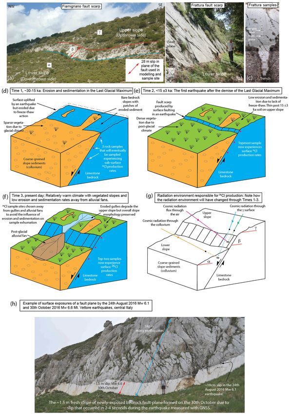
4384                                                                        J. Beck et al.: Bayesian 36 Cl earthquake dating

without thorough modeling of prior beliefs, and proper ac-        to 36 Cl earthquake dating, we extend our model to allow for
counting for parameter and model uncertainties.                   Bayesian regional probabilistic seismic hazard assessment.
   To address these issues, Cowie et al. (2017) used a               We supplement this paper with an easy-to-use MATLAB
Bayesian Markov-chain Monte Carlo (MCMC) sampler                  code of the proposed Bayesian MCMC method for earth-
(Robert and Casella, 2004) to generate ensembles of plausi-       quake dating and regional probabilistic seismic hazard as-
ble solutions. However, the candidate space considered was        sessment.
restricted by the assumption of equally spaced and sized dis-
placements in active slip time periods. Also, priors on the
placement and number of active time periods were not dis-         2   Simulation of 36 Cl concentrations along fault scarps
cussed. Furthermore, their approach did not incorporate un-
                                                                  Typical faults scarps are shown in Fig. 1a–c. These are char-
certainties in important parameters such as the 36 Cl spalla-
                                                                  acterized by two slopes that were originally joined, but are
tion and muonic production rates, the colluvial wedge mean
                                                                  now offset across a geological fault due to surface slip events
density, which is difficult to measure in the field, and the
                                                                  during earthquakes. The original planar slope (see Fig. 1d)
timing of the demise of the Last Glacial Maximum (LGM)
                                                                  was formed during the LGM, which for southern Europe
after which slip was preserved on the fault plane, which is
                                                                  ended around 20 000 to 12 000 years before present (20–
only known imprecisely. Finally, their implementation of the
                                                                  12 ka), through intense erosion on the upthrown side of the
MCMC algorithm was not fully described, and no evidence
                                                                  fault that was subject to freeze-thaw action (frost shatter-
of convergence was shown.
                                                                  ing) and sedimentation of the liberated slope debris (collu-
   The new Bayesian MCMC method proposed in the current
                                                                  vium) on the downthrown side of the fault. Figure 1d–f also
work adopts the Brownian motion model for earthquake re-
                                                                  show how the morphology of the scarp changes through time
currence (Matthews et al., 2002) to form a candidate space
                                                                  across the LGM to post-glacial transition.
for earthquakes that arise and the associated prior probabili-
                                                                     Before the demise of the LGM (see Fig. 1d), erosion via
ties. Besides improving the recurrence of prior earthquakes,
                                                                  freeze-thaw action rapidly removed the surface uplifted by
this enables forecasts of future earthquakes, which is cru-
                                                                  earthquakes (Allen et al., 1999; Peyron et al., 1998). Dur-
cial for the subsequent task of regional seismic hazard as-
                                                                  ing the demise of the LGM, decreasing erosion rates may
sessment (Pace et al., 2006, 2014). Furthermore, we forgo
                                                                  have allowed fault slip to be preserved as a scarp, depending
the unrealistic assumption in Cowie et al. (2017) that all dis-
                                                                  on the relative rates of erosion and fault slip. However, after
placements are of equal size and instead allow sizes to lie
                                                                  the demise the LGM (Fig. 1e), the slip was preserved due to
in a fault-dependent range. We employ parallel tempering
                                                                  low erosion rates relative to the fault slip rates (Roberts and
(Woodard et al., 2009) to avoid premature convergence to
                                                                  Michetti, 2004; Cowie et al., 2013, 2017). The type of slip
local rather than global optima due to a lack of explorative
                                                                  is illustrated in Fig. 1h, which shows decimeter-scale slips
capabilities. We verified the correct implementation of our
                                                                  produced during two earthquakes at the Mt. Vettore fault on
MCMC algorithm by the test of Talts et al. (2018) and mea-
                                                                  24 August 2016 (Mw 6.1) and on 30 October 2016 (Mw 6.6).
sure global convergence with the diagnostic of Gelman and
                                                                  The Mw 6.6 surface rupture formed in 2–4 s during coseis-
Rubin (1992). Since no model of 36 Cl production can be
                                                                  mic slip, recorded by Global Navigation Satellite System re-
completely accurate, we include an estimation of model dis-
                                                                  ceivers placed either side of the fault before the earthquake
crepancy (Rougier, 2007; Rougier et al., 2013; Brynjarsdottir
                                                                  (Wilkinson et al., 2017).
and O’Hagan, 2014), which results in more realistic confi-
                                                                     The preserved fault plane can be sampled above ground
dence bands and may help guide various research efforts to
                                                                  and in excavated trenches. The 36 Cl concentration in a fixed
improve the modeling of 36 Cl accumulation. We also account
                                                                  sample of limestone bedrock evolves according to
for uncertainties in important parameters of the model that
were previously held fixed. More specifically, we assume un-      dg(t)
certain production rates, attenuation lengths, and colluvium            = φ(t) − λg(t),                                      (1)
                                                                   dt
density, and we infer the time during the demise of the LGM
at which the effect of erosion became outpaced by the ground      where g(t) is the 36 Cl concentration (atoms g−1 ), φ(t) is
displacements. We apply our algorithm to a synthetic case to      the production rate (atoms g−1 yr−1 ), and λ is the decay rate
verify the identifiability of past earthquakes in our model.      of 36 Cl (yr−1 ). The main 36 Cl production pathways in pure
   Finally, we study earthquake displacement histories for        limestones are spallation of 40 Ca, muon capture by 40 Ca, and
the Fiamignano and Frattura faults in the Italian Apennines.      thermal neutron capture by 35 Cl (Marrero et al., 2016). These
The results provide new evidence of slip-rate variability in      processes depend on cosmic radiation flux, which is attenu-
normal faults in the Italian Apennines. The timing of slip-       ated by the surrounding environment composed of air, col-
rate episodes can be reconciled with the historical record        luvium, and rock (see Fig. 1g). As a consequence, the pro-
of earthquakes and damage to the Colosseum and other an-          duction rate φ(t) in a rock sample through time is strongly
cient buildings in Rome. Beyond proposing a new approach          influenced by earthquake-induced changes to the surround-
                                                                  ing environment. Roughly speaking, samples taken from the

Geosci. Model Dev., 11, 4383–4397, 2018                                            www.geosci-model-dev.net/11/4383/2018/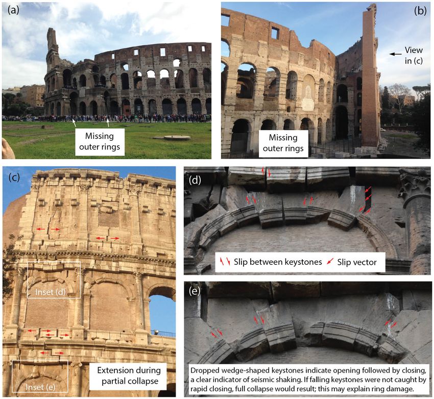
J. Beck et al.: Bayesian 36 Cl earthquake dating                                                                                         4385

trench have experienced 36 Cl production at low rates due to                 – Geological properties:
shielding by overlying colluvium and neighboring limestone
bedrock (see Fig. 1g), whereas aboveground samples have                          – rock mean density, ρrock (g cm−3 );
experienced early subsurface production before exhumation                        – colluvial wedge mean density, ρcoll (g cm−3 );
as well as subsequent surface production. This results in a                      – spallation production rate of 36 Cl by fast sec-
characteristic 36 Cl concentration profile along the fault plane,                  ondary neutrons at the surface from 40 Ca, 9sp
which captures its history of ground displacements. Note                           (atoms g−1 yr−1 );
that samples must be taken from a fault plane away from
post-glacial alluvial fans and eroded gullies where exposure                     – slow muon capture production rate of 36 Cl at the
is also influenced by post-glacial erosion and sedimentation                       surface from 40 Ca, 9µ (atoms g−1 yr−1 );
(see Fig. 1f)                                                                    – neutron apparent attenuation length, 3sp , and muon
   Formulae for surface production through the aforemen-                           apparent attenuation length, 3µ , for a horizontal
tioned processes as well as the associated attenuation, or                         unshielded surface (g cm−2 );
shielding, factors can be found in Gosse and Phillips (2001)                     – chemical compositions (ppm) of the rock in each
and Schlagenhauf et al. (2010). More than a decade of con-                         sample and of the soil and pebbles in the colluvium.
tributions to the modeling of 36 Cl production (Lal, 1988;
Phillips et al., 1996; Mitchell et al., 2001) have been as-                  – Further properties:
sembled into a MATLAB code that computes 36 Cl concen-
                                                                                 – the influence of the geomagnetic field is specified
trations in a set of bedrock samples for given sequences of
                                                                                   through scaling factors for fast neutrons and slow
scarp displacements and event times; the code is provided
                                                                                   muons, see the supplement of Schlagenhauf et al.
in the supplement of Schlagenhauf et al. (2010). The code
                                                                                   (2010);
solves Eq. (1) by a first-order finite-difference scheme, and
uses various simplifications for calculating the shielding fac-                  – the time during the demise of the LGM at which the
tors; for example, it assumes that the cosmic ray flux decays                      effect of erosion became outpaced by the ground
exponentially with the depth of a sample beneath the collu-                        displacements, Tinit (yr−1 ).
vial wedge.
   As part of this work, we provide a MATLAB code that cir-
                                                                         3    Bayesian inference of displacement histories using
cumvents some of the approximations and simplifications of
                                                                              MCMC
Schlagenhauf et al. (2010), in particular in the computation
of shielding factors. We use exact solutions of Eq. (1), piece-          In this section, we present a Bayesian MCMC algorithm
wise exponentials, which is possible under the assumption of             that solves the inverse problem of the previous section,
a constant-in-time production rate. These changes improved               i.e., the inference of past earthquakes from 36 Cl measure-
the predicted 36 Cl concentration by around 5 % in our numer-            ments y = (y1 , . . ., yM ) at M sample sites along a single
ical experiments. Furthermore, we introduce an offline phase             fault scarp. More specifically, we compute posterior distribu-
during which we pre-compute a database of shielding factors              tions for the vectors of fault displacements and event times,
for a sparse grid (Barthelmann et al., 2000) of possible val-            d = (d1 , . . ., dN ) and s = (s1 , . . ., sN ), respectively (and in
ues of the model parameters. By interpolating between these              particular for the number of events, N). In addition, we treat
factors, we were able to accelerate the computations during              the values of z := (Tinit , 9sp , 9µ , 3sp , 3µ , ρcoll ) as uncertain
the inverse problem by 2 orders of magnitude. Finally, an im-            parameters and include them in the inference problem.
provement of particular relevance to our case studies is that               Denoting the vector of true 36 Cl concentrations by y∗ , and
we also consider events before the end of the LGM. We ap-                the output of the computer model of Eq. (2) for given values
proximate the effects of the LGM on erosion in a binary man-             of x := (d, s, z) by g(x), we first observe the equation
ner, by assuming a single point in time, Tinit , before which
erosion immediately eroded scarps formed by earthquakes,                 y = y∗ +  = g(x) + δ + ,                                        (2)
and after which erosion stopped completely.
   The provided MATLAB code calculates 36 Cl concentra-                  where  is the measurement error, i.e., the discrepancy be-
tions in a set of bedrock samples for given sequences d =                tween the true and the measured concentrations, and δ :=
(d1 , . . ., dN ) and s = (s1 , . . ., sN ) of scarp displacements and   y∗ − g(x) is the model error, i.e., the discrepancy between
event times and the following fault site properties.                     the model output and the true concentrations (Rougier et al.,
                                                                         2013; Brynjarsdottir and O’Hagan, 2014). We assume that
  – Geometric description (see Fig. 1g):                                 the measurement errors are independent and normally dis-
       – dip of the lower slope, α (◦ );                                 tributed,  ∼ N (0, σ 2 ) for a given vector σ = (σ1 , . . ., σM )
                                                                         of positive real numbers. The model error is assumed to be
       – fault plane dip, β (◦ );                                        proportional to the measurements, δ ∼ N (0, (ρy)2 ), and we
       – dip of the upper slope of the footwall, γ (◦ );                 include the value of ρ > 0 in the inference problem.

www.geosci-model-dev.net/11/4383/2018/                                                       Geosci. Model Dev., 11, 4383–4397, 2018
4386 J. Beck et al.: Bayesian 36 Cl earthquake dating Figure 1. Images and illustrations of scarp evolution and radiation environment. Geosci. Model Dev., 11, 4383–4397, 2018 www.geosci-model-dev.net/11/4383/2018/
J. Beck et al.: Bayesian 36 Cl earthquake dating                                                                                     4387

   To describe the Bayesian inference method, let us denote               (BPT) distribution since it describes the time required for a
the vector of all unknowns by θ := (x, ρ, φ), where φ con-                Brownian motion to reach a certain threshold. To account
tains auxiliary variables that are described in Sect. 3.1 below.          for large-scale time periods with differing average earth-
If we have a prior belief on the value of θ , described by a              quake frequencies, we extend the model in Matthews et al.
probability distribution Pθ , then the posterior distribution for         (2002) by including a Poisson (3 Tmin )-distributed number
θ given the measurements y can be found using Bayes’ rule,                J of switch points (tj )Jj=1 , where tj ∼ U([−Tmin , 0]) and
                                                                          3 ∼ U([10−4 , 10−3 ]). This is equivalent to the assumption
Pθ |y ∝ Py|θ Pθ ,                                                  (3)
                                                                          that the times between successive switch points are exponen-
with the distribution of y conditioned on a fixed value of θ ,            tial random variables whose mean 1/3 is inferred in the in-
or likelihood, given by                                                   terval [103 , 104 ]. We then define the drift a(t) and volatility
                                                                          b(t) of the Brownian motion in the intervals of the resulting
Py|θ ∼ N (g(x), σ 2 + (ρy)2 ).                                            partition of [−Tmin , 0] by
To gain information about the posterior distribution Pθ |y , we           (a(t), b(t)2 ) := (1/νj , τ 2 /νj ) for tj ≤ t ≤ tj +1
employ a MCMC method (Robert and Casella, 2004), which
                                                                          (with t0 := −Tmin and tJ +1 := 0),                           (4)
generates samples that, roughly speaking, behave as if they
were drawn from the posterior and thus can be used to ap-
                                                                          where the average interarrival times ν = (νj )Jj=0 are inde-
proximate statistical properties thereof. More specifically, we
                                                                          pendent and identically distributed according to an inverse
use a Metropolis–Hastings MCMC method, which generates
                                                                          gamma distribution with mean m ∼ U([200, 2000]) and
a sequence (chain) (θ k )∞
                         k=1 of random samples, where an ini-             shape parameter α ∼ U([1, 10]), and where τ ∼ U([0, 1])
tial sample is taken from the prior distribution and each suc-
                                                                          controls the short-scale recurrence variability (with the above
cessive sample is generated from its predecessor by means
                                                                          definitions, the standard deviation of interarrival times in the
of random proposal functions and an acceptance step that
                                                                          j th subinterval is τ νj ). Numerically, given values of ν and
guarantees that the distribution of θ k converges to the de-
                                                                          τ , we use forward Euler–Maruyama time stepping (Higham,
sired distribution Pθ |y as k → ∞. To accelerate this conver-
                                                                          2001) with time discretization 1t ≈ 15 (yr−1 ) to simulate the
gence, we employ a parallel tempering approach that simul-
                                       (l)                                resulting stochastic process on [−Tmin , 0], with the modifica-
taneously generates L > 1 chains (θ k )∞   k=1 , 1 ≤ l ≤ L with           tion that we reset the process to 0, and generate an earthquake
progressively flattened likelihood distributions,
                                                                          by extending d and s, each time it reaches the threshold 1. In
  (l)
Py|θ ∼ N (g(θ ), κl (σ 2 + (ρy)2 )), 1 = κ1 < . . . < κl < . . . < κL ,   formulae, we let

and randomly swaps states between neighboring chains such                 X̂i+1 := Xi + a(i1t)1t + b(j 1t)Wi+1 ,
                                                 (1)
that the resulting samples of the first chain (θ k )∞k=1 , which
                                                                                   (
                                                                                    X̂i+1 if X̂i+1 < 1,
uses κ1 = 1, are still distributed according to Pθ |y (in the             Xi+1 :=                                                      (5)
limit). This has been shown to accelerate the exploration of                        0 otherwise.
the state space in cases where the posterior distribution has
multiple local maxima (Woodard et al., 2009).                             The values Wi ∼ N (0, 1t) together with ν and τ and the ini-
   To fully specify our inference method, it remains to de-               tial value X0 ∼ U([0, 1]) form the vector of auxiliary vari-
scribe the prior distribution Pθ and the proposal functions               ables φ referred to above, which fully determines the process
                                                                               Tmin /1t
that are used for sample generation.                                      (Xi )i=0      , which in turn determines the vector of earth-
                                                                          quake times s.
3.1     The prior distribution Pθ                                            For the prior distribution of the displacement vector d con-
                                                                          ditioned on the number N of earthquake events, we use a
We describe the prior distributions of different components               uniform prior on the hypercube
                                                                                                  PN         [dmin , dmax ]N conditioned on
of θ with the understanding that separately described com-                the requirement that n=1 dn = Hsc , where Hsc (see Fig. 1)
ponents are assumed to be stochastically independent.                     is the present height of the fault scarp, and dmin and dmax are
   For the parameter ρ, which controls the relative model er-             fault-dependent bounds on displacement sizes.
ror, we assume a uniform prior distribution, ρ ∼ U[0, ρmax =                 Finally, we assign prior distributions to the components
0.1].                                                                     of z: Tinit ∼ U([12 000, 20 000]), 9sp ∼ N (48.8, 1.7),
   To describe a prior for the earthquake times s (and in par-            9µ ∼ N (190, 19), 3sp ∼ U([180, 220]), and 3µ ∼
ticular the number of events N), we extend our state space                U([1300, 1700]), where the first three are based on re-
by a stochastic process in [−Tmin , 0] that is used to model              sults of Allen et al. (1999), Stone et al. (1996), and Heisinger
earthquake occurrence (see Fig. 2). In doing so, we fol-                  et al. (2002), respectively, and the remaining are chosen to
low Matthews et al. (2002), where the time between suc-                   be uniform around values taken from Schlagenhauf et al.
cessive earthquakes is modeled by an inverse Gaussian dis-                (2010). It is difficult to accurately measure the value of
tribution, which is also called the Brownian passage-time                 ρcoll in the field due to compaction of the sediment during

www.geosci-model-dev.net/11/4383/2018/                                                        Geosci. Model Dev., 11, 4383–4397, 2018
4388 J. Beck et al.: Bayesian 36 Cl earthquake dating
Figure 2. Sample path of stochastic process used for earthquake event time generation. Sample path generated with X0 = 0.16, Tmin =
−30 kyr, t1 = −10 kyr, ν = (15 kyr, 3 kyr), τ = 0.5, and 1t ≈ 0.007 kyr. The corresponding earthquake times are represented by dots on the
time axis, the switch point t1 is represented by a red vertical line.
current value. To propose the partition of [−Tmin , 0] and the
corresponding piecewise constant drift and volatility coeffi-
cients, we employ reversible jump MCMC (Green, 1995),
which allows for the application of MCMC to variables
whose state space contains subspaces of different dimension-
Tmin /1t
ality. To propose new values of the variables (Wi )i=1 ,
Tmin /1t
which drive the process (Xi )i=1 , we again use a global
proposal, which redraws all values independently, as well
as a Brownian bridge-type local proposal that redraws the
values within a random subinterval of [−Tmin , 0] from their
prior distribution conditioned on maintaining their sum. If a
proposal changes the number of earthquakes, the earthquake
displacement vector d (which then has a different size) is re-
sampled too, and if a proposal changes the number of switch
points, the vectors of drift and volatility coefficients are re-
sampled as well.
4 Application to synthetic 36 Cl data
In this section we apply our Bayesian MCMC method to
Figure 3. Measured and sampled 36 Cl concentrations for the syn- synthetic 36 Cl data. To generate these data, we drew d and
thetic case with 146 36 Cl measurements s from the prior distributions described in Sect. 3.1 with
dmin = 10 (cm) and dmax = 110 (cm) and applied the com-
excavation of the sample trench at the base of the fault scarp, puter model of Sect. 2 using the chemical compositions of
so we adopt the relatively wide prior ρcoll ∼ U([1.2, 1.8]) 146 rock samples from the Fiamignano fault (Cowie et al.,
for all case studies considered in this work. 2017) and the values z = (Tinit = −19000, 9sp = 49.5, 9µ =
200, 3sp = 195, 3µ = 1700, ρcoll = 1.6). The remaining pa-
3.2 MCMC proposal functions rameters, which are not part of the inference problem, were
chosen as Hsc = 2705, Htr = 115, ρrock = 2.7, α = 23, β =
To explore the state space, we design a number of proposal 42, and γ = 33, based on the true values of the Fiamignano
functions and apply a subset of these before each rejection fault that were measured in the field. Finally, we perturbed
step in the MCMC algorithm. For each component of z as the 36 Cl concentration values according to Eq. (2), with stan-
well as for the values of ρ, ν, τ , and X0 , we include a global dard deviation σ = 0.025g(x) for the measurement error and
proposal from the corresponding prior distribution as well as ρ = 0.03 in the model error term. The realizations of d and s
a local proposal based on a normal distribution around the are given in the Supplement.
Geosci. Model Dev., 11, 4383–4397, 2018 www.geosci-model-dev.net/11/4383/2018/J. Beck et al.: Bayesian 36 Cl earthquake dating 4389
Figure 4. The synthetic case with 146 36 Cl measurements: the accumulated displacement (a), the mean earthquake intensity (b), and an
event scatter plot (c) showing true events (blue) and events from posterior samples (with gray scale to indicate frequencies).
Figure 5. Gelman–Rubin diagnostic for the synthetic case with 146
36 Cl measurements Figure 6. Measured and sampled 36 Cl concentrations for the syn-
thetic case with 16 36 Cl measurements
We ran our MCMC method using the priors speci-
fied in Sect. 3.1 for the uncertain parameters, i.e., Tinit ∼ a 10 % burn-in period. Among these samples were 843 735
U([12 000, 20 000]), 9sp ∼ N (48.8, 1.7), 9µ ∼ N (190, 19), distinct scenarios, whose repetitions correspond to rejected
3sp ∼ U([180, 220]), and 3µ ∼ U([1300, 1700]), ρcoll ∼ proposals and reflect their statistical weight. Finally, to accel-
U([1.2, 1.8]). erate post-processing and to decrease memory consumption,
The results presented in this section are based on two in- we only saved each fifth scenario together with its number of
dependent MCMC chains, each consisting of L = 20 parallel repetitions (thinning).
tempering levels. We performed 1 374 462 MCMC iterations Figure 3 shows that the medians of the 36 Cl concentra-
of each chain, resulting in a combined number of 2 474 032 tions of the posterior samples provide a good fit to the syn-
samples in the first levels of the two independent chains after thetic measured concentrations. More importantly, Fig. 4a
www.geosci-model-dev.net/11/4383/2018/ Geosci. Model Dev., 11, 4383–4397, 20184390 J. Beck et al.: Bayesian 36 Cl earthquake dating
Figure 7. The synthetic case with 16 36 Cl measurements: the accumulated displacement (a), the mean earthquake intensity (b), and an event
scatter plot (c) showing true events (blue) and events from posterior samples (with gray scale to indicate frequencies).
Figure 8. Location map of the central Apennines and the Fi-
amignano and Frattura sample sites. Holocene active faults and his-
torical ruptures adapted from Roberts and Michetti (2004), Pace Figure 9. Damage to the Colosseum in Rome.
et al. (2006), Cowie et al. (2017), and Mildon et al. (2017).
means that individual events in that period cannot be recov-
shows that the posterior median of the accumulated displace- ered. Nevertheless, including such events in our approach can
ment is close to the true value throughout the entire time be considered a way to obtain realistic prior 36 Cl concentra-
span. This indicates that past earthquake activity can be re- tions at the end of the LGM, Tinit , as opposed to the alter-
covered despite measurement errors (here 2.5 %), model er- native to start with zero concentrations or imposing ad hoc
rors (here 3 %), and parameter uncertainties. Figure 4 (b, c) pre-exposure times (Schlagenhauf et al., 2010).
shows the posterior mean earthquake intensity, i.e., the av- Figure 5 shows the convergence diagnostic of Gelman and
erage displacement per time (computed for bins of width Rubin (1992). The potential scale reduction factor (PSRF)
∼ 500 years), and a scatter plot of all earthquake events of associated with the accumulated displacement values of
the posterior samples. Fig. 4 is less than 1.08.
In both plots, the erosion during the LGM has removed in- Since the collection and chemical analysis of 36 Cl samples
formation and so leads to almost uniform posterior intensities involve time-consuming and costly fieldwork and lab work,
across time and through event sizes during the LGM, which in particular the accelerator mass spectrometry (AMS) anal-
Geosci. Model Dev., 11, 4383–4397, 2018 www.geosci-model-dev.net/11/4383/2018/J. Beck et al.: Bayesian 36 Cl earthquake dating 4391
up to 2–2.5 km, which means long-term rates of vertical mo-
tion across the faults are in the order of 0.1 cm yr−1 .
In this section we apply our method to the Fiamignano and
Frattura faults of the Italian Apennines, and show its appli-
cability to regional probabilistic seismic hazard assessments.
5.1 Fiamignano fault
The Fiamignano fault is located on the southwest flanks
of the Apennines, approximately 60 km northeast of Rome.
Based on a study of 34 damaging earthquakes recorded in
Guidoboni et al. (2007), Galli and Molin (2014), and Vittori
(2015), intensity VIII damage is expected at distances of less
than ∼ 40–60 km of an epicenter from a Mw ∼ 6.0–6.5 event,
and the Fiamignano fault is one of the few Apennine normal
faults with that epicentral distance to Rome (see Fig. 8) thus
making it a plausible source of the historic earthquake dam-
age.
Rome was damaged in earthquakes of intensity VIII dur-
ing at least three earthquakes in the 5th, 9th, and 14th cen-
turies. Other earthquakes damaged the city in AD 801, 1091,
Figure 10. Fiamignano fault: measured and sampled 36 Cl concen- 1231, 1279, 1298, 1328 (Guidoboni et al., 2007). The Colos-
trations.
seum was damaged in AD 484 or 508 based on a stone in-
scription where a person known as “Decius Marius Venan-
tius Basilus,” a prefect of the city, declares that he directly
ysis, it is worthwhile knowing whether fewer than 146 sam- paid for restoration works after an earthquake; the uncer-
ples can provide similar insights. To answer this question, we tainty in age is because two Decius’ who were consul, one
repeated our computations with a subset of 16 rock samples in AD 484 and another in AD 508. Damage consisted of col-
(see Fig. 6). lapse of the colonnades in the summa cavea (upper seat-
Figure 7 shows that this reduced dataset leads to similar ing section for plebian spectators) with major damage to the
results as the complete dataset (cf. Fig. 4). These results are arena and podium. Collapse of the outer rings of the Colos-
based on 421 022 MCMC iterations of each chain and using seum is sometimes attributed to an AD 847 earthquake, when
the same number of chains, burn-in, and thinning as before, the nearby church of Santa Maria Antiqua was abandoned
which led to a maximal PSRF value of 1.02. after earthquake damage (Vittori, 2015). An earthquake also
damaged Rome on 9 September AD 1349, one of three large
earthquakes in the Apennines on that day. This earthquake is
5 Application to normal faults in the Italian Apennines thought to be linked to the Fiamignano fault based on the
observation that taxes were reduced in the vicinity of the
The Italian Apennines contain many examples of bedrock Fiamignano fault due to misery and depopulation after the
scarps on active normal faults and it has been suggested that earthquake (Guerrieri et al., 2002). Damage and collapse re-
rates of slip produced by repeated earthquake rupture since ported in 14th century accounts are summarized in Galli and
the LGM can be used to investigate seismic hazards and the Molin (2014), where the earthquake on that day is described
mechanics of continental deformation (Piccardi et al., 1999; as “the strongest seismic shaking ever felt in Rome” (Galli
Roberts and Michetti, 2004; Cowie et al., 2013). The ac- and Molin, 2014). It is postulated that there was an abrupt
tive normal faults work to extend the continental crust at collapse of the southern external ring of the Colosseum dur-
the present day in formerly thickened crust of the Alpine– ing this earthquake, as observed in Fig. 9, because a bull fight
Apennines collision zone. The extension started at 2–3 Ma, was hosted there in AD 1332, suggesting the Colosseum was
as evidenced by dated sediments in extensional sedimentary intact, and an announcement that the collapsed stones were
basins formed by fault activity (Cavinato and Celles, 1999; for sale was made in the second half of the 14th century. Fur-
Roberts et al., 2002). The basins occur on the downthrown thermore, an intact Colosseum can be seen on a coin from
side of the faults, and contain accumulations of sedimentary AD 1328, whereas a damaged Colosseum is displayed on a
layers that are usually hundreds to a few thousand meters 15th century image (Galli and Molin, 2014). Minor damage
thick. When added to the offset implied by the uplifted moun- to the Colosseum also occurred in an AD 1703 earthquake
tains on the upthrown side of the faults, total fault offsets are (Vittori, 2015).
www.geosci-model-dev.net/11/4383/2018/ Geosci. Model Dev., 11, 4383–4397, 20184392 J. Beck et al.: Bayesian 36 Cl earthquake dating Figure 11. Fiamignano fault: the accumulated displacement (a), the mean earthquake intensity (b) and an event scatter plot (c) showing events from posterior samples (with gray scale to indicate frequencies). Figure 12. Fiamignano fault: detailed view of posterior displacement history and earthquake intensity. The vertical blue lines show the timings of two events that damaged the Colosseum. One of the goals of this work is to investigate whether In our analysis, we use the same site parameter values and the Fiamignano fault is a candidate for the historical damage priors as in Sect. 4 except that we now use dmax = 300, moti- accounts in Rome based solely on 36 Cl analysis. 36 Cl data vated by the large displacements for similar faults presented from the Fiamignano fault have previously been collected in Wells and Coppersmith (1994). We performed 1 311 016 and analyzed in Cowie et al. (2017), where geomorphic and MCMC iterations of each chain and used the same num- structural field mapping as well as laser and radar datasets ber of chains, the same burn-in, and thinning as in the syn- was presented as evidence that their site was exhumed by thetic case. A maximal PSRF value of 1.03 using two inde- tectonic slip as opposed to exhumation by erosion. Cowie pendent MCMC chains indicates convergence. The minimal et al. (2017) tried to infer an earthquake history for the fault, weighted root mean squared error (wRMS) among all sce- and the results suggest rapid displacement between approx- narios was 1.42. The time required for the offline calcula- imately 2000 years ago and AD 1349. However, the results tions was ∼ 15 min and the total time was ∼ 12 days. In this were biased by the modeling constraint that the most recent work, we performed all numerical experiments on Intel Xeon earthquake was enforced to be at AD 1349 and by the use E5-2680 v2 at 2.80 GHz (20 cores) with MATLAB (2016a). of constant inter-event times between slip-rate change points The sampled posterior 36 Cl concentrations fit well to the and constant displacement sizes. measurements as observed in Fig. 10. Geosci. Model Dev., 11, 4383–4397, 2018 www.geosci-model-dev.net/11/4383/2018/
J. Beck et al.: Bayesian 36 Cl earthquake dating                                                                                 4393

                                                                     presented as evidence that their site was exhumed by tectonic
                                                                     slip as opposed to exhumation by erosion. Unlike for the Fi-
                                                                     amignano fault, the 36 Cl data were collected sparsely (15
                                                                     samples), similar to the situation in our synthetic case with
                                                                     a reduced amount of data shown. The site-specific parame-
                                                                     ters for the Frattura fault are α = 25, β = 53, and γ = 28;
                                                                     fault scarp height Hsc = 1570, trench depth Htr = 130; and
                                                                     the rock mean density ρrock = 2.7. Here the maximum dis-
                                                                     placement size is again chosen conservatively as dmax = 300;
                                                                     though we mainly expect displacement sizes less than 100 cm
                                                                     based on the data of Wells and Coppersmith (1994). As in the
                                                                     previous cases, we let ρcoll ∼ U([1.2, 1.8]).
                                                                        There are no known historical earthquakes for this fault
                                                                     consistent with records from towns and cities nearby, such as
                                                                     Sulmona and Pescasseroli, for which earthquake records ex-
                                                                     tend back to Roman times. Indeed, the record is thought to be
                                                                     complete since AD 1349 for magnitudes larger than Mw 5.8;
                                                                     see Guerrieri et al. (2002), Guidoboni et al. (2007), Pace et al.
                                                                     (2006), and Roberts and Michetti (2004) for discussions of
                                                                     the completeness period.
                                                                        We performed 522 560 MCMC iterations of each chain
                                                                     and used the same number of chains, burn-in and thinning
Figure 13. Frattura fault: measured and sampled 36 Cl concentra-     as in the synthetic case. A maximal PSRF value of 1.003 in-
tions.                                                               dicates convergence of the MCMC algorithm. The minimal
                                                                     wRMS among all scenarios was 1.78. The same settings are
                                                                     used for the offline calculations (∼ 15 min) and the total time
   Our results agree with Cowie et al. (2017) in that we find        was ∼ 3 days.
clear evidence of slip-rate variability and the slip rate increas-      Figure 14 suggests a scarp age at approximately 19 ka
ing through time before cessation of slip in the last 600–           consistent with expected slope stabilization ages, which may
700 years. Although the present 28 m offset in the plane of          well be the marker for the time of the demise of the LGM
the fault occurred at an average slip rate of ∼ 0.2 cm yr−1 ,        shown in Fig. 1. After ∼ 19 ka, Figs. 14 and 15 indicate
we find rapid slip of 1–1.4 cm yr−1 centered around 1 ka (see        highly variable slip rates throughout the investigated time
Fig. 11). A detailed view for the period from 5 ka to present is     domain: initially a constant moderately high slip rate until
shown in Fig. 12, where we observe that both of the two ma-          ∼ 15 ka, a decreasing slip rate until ∼ 8 ka, a sudden peak
jor earthquake events to have been observed in AD 847 and            in slip from ∼ 5 to 3 ka, and a low occurrence probability
1349 fall within this region of high intensity, see Fig. 12, and     of earthquake events in the past ∼ 2500 years. The lack of
potentially large displacements indicated by dark gray re-           earthquakes in the past ∼ 2500 years is consistent with his-
gions in Fig. 11c. In fact, even the AD 801, 1091, 1231, 1279,       torical earthquake records, which show no major earthquakes
1298, and 1328 earthquakes fall within the high-intensity re-        in the vicinity.
gion at times when our findings suggest relatively low dis-             The displacement histories of the Fiamignano and Frattura
placement sizes. This deserves further investigation, and we         faults provide insights into slip-rate variability. The relatively
hope it leads to paleoseismic studies of offset late Holocene        short-lived bursts of high activity observed in our results oc-
sediments on the Fiamignano fault that may be able to verify         cur at different times on faults in the same tectonic setting.
or refute these possibilities.                                       This suggests that this is not a regional pulse of synchronous
   In conclusion, our findings suggest that slip is highly clus-     high slip, but probably related to the dynamics of interaction
tered in time and that the Fiamignano fault is a plausible           between each fault and its neighbors (Cowie et al., 2012),
source of the AD 847 and 1349 earthquakes associated with            and that slip is highly clustered in time, which has important
damage to the Colosseum and other ancient buildings known            implications for forecasting seismic hazards as discussed be-
from the historical record.                                          low.

5.2     Frattura fault                                               5.3   Application to regional probabilistic seismic hazard
                                                                           assessment
36 Cl data for the Frattura fault have been collected and an-
alyzed in Cowie et al. (2017), where geomorphic and struc-           Our results show that calculating probabilistic seismic hazard
tural field mapping as well as laser and radar datasets was          is considerably more challenging than previously thought.

www.geosci-model-dev.net/11/4383/2018/                                                  Geosci. Model Dev., 11, 4383–4397, 2018
4394 J. Beck et al.: Bayesian 36 Cl earthquake dating Figure 14. Frattura fault: the accumulated displacement (a), the mean earthquake intensity (b) and an event scatter plot (c) showing events from posterior samples (with gray scale to indicate frequencies). Figure 15. Frattura fault: detailed view of posterior displacement history and earthquake intensity. Typical fault-based and time-dependent seismic hazard mod- – a Brownian motion with time-varying drift and noise – into els are based on the BPT distribution and require specifi- the future, which enables us to sample more realistic next cation of the most recent earthquake time, the mean inter- earthquake event times. More specifically, for each of our event time, and the coefficient of variation (CV) value (stan- posterior samples, we continue the simulation of the corre- dard deviation of inter-event times divided by the mean inter- sponding Brownian motion sample path (such as that shown event time) to factor in variability in the inter-event time in Fig. 2) until another earthquake is generated. For this pur- (Pace et al., 2016). However, our results show that in ad- pose, we use the sample-dependent values of the parameters dition to the variability in inter-event times around a con- describing the behavior of the Brownian motion: the aver- stant slip rate, faults show heightened activity and quies- age time 1/3 between large-scale changes in slip activity, cence over time periods lasting a few millennia relative to the small-scale recurrence variability τ , and the hyperparam- the longer-term deformation rate. The differences in slip rate eters α and m that describe the distribution of average inter- between time of heightened activity (> 1 cm yr−1 ) and qui- arrival times in new slip activity periods. Thus, our approach escence (< 0.1 cm yr−1 ) are dramatic. These two timescales is a natural extension of the state-of-the-art methodology that of slip-rate variability are not considered by current meth- accounts for large-scale slip-rate variability and informs the ods for calculating probabilistic seismic hazard (Pace et al., resulting more complex model by the full displacement his- 2006, 2016; Tesson et al., 2016). To address this omission, tory at a given fault site. we extend our more complex earthquake recurrence process Geosci. Model Dev., 11, 4383–4397, 2018 www.geosci-model-dev.net/11/4383/2018/
J. Beck et al.: Bayesian 36 Cl earthquake dating                                                                              4395

Figure 16. Posteriors of next earthquake time for Fiamignano (a) and Frattura (b) according to BED with dmin = 10 and dmin = 50, and
according to a hybrid BED-BPT approach (with dmin = 10 in the BED part).

   Posteriors of the next earthquake time for the Fiamignano           However, a note of caution is that these results are prob-
and Frattura faults are shown in Fig. 16. For comparison, we        ably only meaningful for near-future prediction. A physical
show results based on dmin = 10 and dmin = 50. As expected,         basis that explains the cause of the slip-rate variability re-
the assumption that only earthquakes with a slip larger than        sulting from fault interaction would further improve proba-
50 cm can occur at a given fault reduces the total number           bilistic hazard analysis, as mentioned in Tesson et al. (2016).
of earthquakes and thus the predicted hazard of an impend-          During and after rupture, stress is transferred onto neighbor-
ing future earthquake. Furthermore, we include the results          ing faults, and this is thought to produce a temporal variation
of a hybrid BED-BPT approach that uses the results of our           in slip rate on faults that manifests itself in terms of tempo-
MCMC algorithm but neglects different timescales of slip-           ral earthquake clustering (Scholz, 2010; Cowie et al., 2012;
rate variability in future event time simulations. (Since typ-      Mildon et al., 2017). Interaction allows the fault systems to
ical historical earthquake records are too sparse to provide        share out the work associated with deforming a region be-
realistic estimates of inter-event times and CV values, a pure      tween different faults so that only a few of the total number
BPT approach based on historical earthquake records would           of active faults take part in regional deformation on millen-
vastly underestimate seismic hazard.) For this purpose, we          nial timescales (Cowie et al., 2012). Further work, including
randomly generate a future event time from the BPT distri-          36 Cl results from many faults in the same region, is needed

bution, conditioned on the event occurring in the future, for       to elucidate such interaction.
each sample of our MCMC algorithm, using the mean inter-
event time, CV value, and the most recent event time of that
sample. Figure 16 shows that the effect of predicting future        6   Conclusions
events with the BPT distribution is similar to that of using
dmin = 50. While the latter underestimates the number of past       This work provides a validation of the 36 Cl approach to in-
earthquakes, the former underestimates the chance of a fault        ference of earthquake occurrence from the demise of the
becoming active despite recent inactivity.                          LGM until present. We propose a Bayesian MCMC method
   An important finding is that the values differ between the       for the study of earthquake displacement histories, with ap-
two faults, and with measurement data from more faults it           plications to regional probabilistic hazard assessment. The
would be of great interest to map such posteriors across en-        method improves on the 36 Cl modeling in Schlagenhauf et al.
tire regions such as that shown in Fig. 8. We expect site-          (2010), the Bayesian inference for 36 Cl earthquake recovery
specific values for these posteriors to change on a length          in Cowie et al. (2017), and the regional probabilistic hazard
scale of 20–30 km, the length of individual faults. Thus, our       assessment in Pace et al. (2006) and Tesson et al. (2016).
approach facilitates high spatial resolution seismic hazard         After demonstrating identifiability in the inverse problem
mapping by implicitly including individual seismic sources          through a synthetic case study, we present probabilistic earth-
(active/capable faults), the long-term slip rates, and impor-       quake displacement histories for the Fiamignano and Frattura
tantly the two timescales of slip-rate variability (millennial-     faults in the Italian Apennines. We obtain highly variable slip
scale heightened activity or quiescence, and inter-earthquake       rates at both faults, in agreement with earlier studies of the
time variability).                                                  region. At the Fiamignano fault, our findings suggest slip in
                                                                    earthquakes at times when the Colosseum and other ancient

www.geosci-model-dev.net/11/4383/2018/                                                 Geosci. Model Dev., 11, 4383–4397, 2018
4396 J. Beck et al.: Bayesian 36 Cl earthquake dating
buildings in Rome were damaged. Conversely, at the Frat- Nowaczyk, N. R., Watts, W. A., Wulf, S., Zolitschka, B., Hub-
tura fault, our result is consistent with the fact that no large berten, H.-W., and Oberhänsli, H.: Rapid environmental changes
earthquakes were reported since Roman times. in southern Europe during the last glacial period, Nature, 400,
740–743, 1999.
Barthelmann, V., Novak, E., and Ritter, K.: High dimensional poly-
Code availability. The MATLAB code Bayesian Earthquake Dat- nomial interpolation on sparse grids, Adv. Comput. Mathe., 12,
ing (BED) v1.0.1 of our Bayesian MCMC method for 36 Cl earth- 273–288, 2000.
quake dating and regional probabilistic seismic hazard assessment Beck, J., Wolfers, S., and Roberts, G. P.: Bayesian
and the data required to reproduce our results are available as Sup- Earthquake Dating (BED) (Version 1.0.1), Zenodo,
plement and at https://doi.org/10.5281/zenodo.1402093 (Beck et https://doi.org/10.5281/zenodo.1402093, 2018.
al., 2018). Future releases of BED can be found at https://github. Benedetti, L., Finkel, R., Papanastassiou, D., King, G., Armijo, R.,
com/beckjh/bed36Cl (last access: 22 August 2018; Beck et al., Ryerson, F., Farber, D., and Flerit, F.: Post-glacial slip history of
2018). the Sparta fault (Greece) determined by 36Cl cosmogenic dating:
evidence for non-periodic earthquakes, Geophys. Res. Lett., 29,
1–4, https://doi.org/10.1029/2001GL014510, 2002.
Brynjarsdottir, J. and O’Hagan, A.: Learning about physical param-
The Supplement related to this article is available eters: the importance of model discrepancy, Inverse Prob., 30,
online at: https://doi.org/10.5194/gmd-11-4383-2018- 114007, https://doi.org/10.1088/0266-5611/30/11/114007, 2014.
supplement Cavinato, G. and Celles, P. D.: Extensional basins in the tectoni-
cally bimodal central Apennines fold-thrust belt, Italy: response
to corner flow above a subducting slab in retrograde motion, Ge-
Author contributions. JB and SW developed and implemented the ology, 27, 955–958, 1999.
MCMC algorithm. All authors contributed to the underlying statis- Cowie, P., Scholz, C., Roberts, G. P., Walker, J. F., and
tical modeling and the 36 Cl simulation itself. JB was the main au- Steer, P.: Viscous roots of active seismogenic faults re-
thor of the manuscript with SW authoring Sect. 3. GPR contributed vealed by geologic slip rate variations, Nat. Geosci., 6, 1036,
with an in-depth description of the physical problem with the cor- https://doi.org/10.1038/NGEO1991, 2013.
responding figures, co-wrote the introduction, collated the informa- Cowie, P. A., Phillips, R. J., Roberts, G. P., McCaffrey, K., Zi-
tion on the historical accounts, and provided geological and seismo- jerveld, L. J. J., Gregory, L. C., Faure Walker, J., Wedmore, L.
logical interpretation of the results. N. J., Dunai, T. J., Binnie, S. A., Freeman, S. P. H. T., Wilcken,
K., Shanks, R. P., Huismans, R. S., Papanikolaou, I., Michetti, A.
M., and Wilkinson, M.: Orogen-scale uplift in the central Italian
Apennines drives episodic behaviour of earthquake faults, Tech.
Competing interests. The authors declare that they have no conflict
Rep. 44858, 2017.
of interest.
Cowie, P. A., Roberts, G. P., Bull, J. M., and Visini, F.: Relationships
between fault geometry, slip rate variability and earthquake re-
currence in extensional settings, Geophys. J. Int., 189, 143–160,
Acknowledgements. This work was supported by NERC directed 2012.
grant NE/J017434/1 “Probability, Uncertainty and Risk in the Galli, P. A. and Molin, D.: Beyond the damage threshold: the his-
Environment”, NERC standard grant NE/I024127/1 “Earthquake toric earthquakes of Rome, B. Earthq. Eng., 12, 1277–1306,
hazard from 36-Cl exposure dating of elapsed time and Coulomb 2014.
stress transfer”, NERC standard grant NE/E016545/1, “Testing Gelman, A. and Rubin, D. B.: Inference from iterative simulation
Theoretical Models for Earthquake Clustering using 36Cl Cos- using multiple sequences, Stat. Sci., 7, 457–472, 1992.
mogenic Exposure Dating of Active Normal Faults in Central Gosse, J. C. and Phillips, F. M.: Terrestrial in situ cosmogenic nu-
Italy”, and the KAUST Office of Sponsored Research (OSR) under clides: theory and application, Quaternary Sci. Rev., 20, 1475–
award no. URF/1/2584-01-01. We thank the many participants in 1560, 2001.
these grants for discussions on earthquakes and 36 Cl, although the Green, P. J.: Reversible jump Markov chain Monte Carlo compu-
views expressed in this paper are our own and any misconceptions tation and Bayesian model determination, Biometrika, 82, 711–
are our sole responsibility. Francesco Iezzi kindly provided the 732, 1995.
field photograph in Fig. 1h. Eutizio Vittori kindly advised on Guerrieri, L., Pascarella, F., Silvestri, S., and Serva, L.: Evoluzione
interpretations of earthquake damage to buildings in Rome. recente dea paesaggio e dissesto geologico-idraulico: primo
risultati in un’area campione dell’Appennino Centrale (valle del
Edited by: Thomas Poulet Salto–Rieti), Boll. Soc. Geol. Ital, 57, 453–461, 2002.
Reviewed by: Bruno Pace and one anonymous referee Guidoboni, E., Ferrari, G., Mariotti, D., Comastri, A., Tarabusi,
G., and Valensise, G.: Catalogue of Strong Earthquakes in Italy
(461 BC-1997) and Mediterranean Area (760 BC-1500), avail-
able at: http://storing.ingv.it/cfti4med/ (last access: 22 October
References 2018), 2007.
Heisinger, B., Lal, D., Jull, A., Kubik, P., Ivy-Ochs, S., Knie, K.,
Allen, J. R. M., Brandt, U., Brauer, A., Huntley, B., Keller, J., and Nolte, E.: Production of selected cosmogenic radionuclides
Kraml, M., Mackensen, A., Mingram, J., Negendank, J. F. W.,
Geosci. Model Dev., 11, 4383–4397, 2018 www.geosci-model-dev.net/11/4383/2018/J. Beck et al.: Bayesian 36 Cl earthquake dating 4397 by muons: 2. Capture of negative muons, Earth Planet. Sci. Lett., Rougier, J.: Probabilistic inference for future climate using an en- 200, 357–369, 2002. semble of climate model evaluations, Clim. Change, 81, 247– Higham, D. J.: An algorithmic introduction to numerical simula- 264, 2007. tion of stochastic differential equations, SIAM Rev., 43, 525– Rougier, J., Sparks, S., and Hill, L. J.: Risk and Uncertainty Assess- 546, 2001. ment for Natural Hazards, Cambridge University Press, 2013. Lal, D.: In situ-produced cosmogenic isotopes in terrestrial rocks, Schlagenhauf, A., Gaudemer, Y., Benedetti, L., Manighetti, I., Annu. Rev. Earth Planet. Sci., 16, 355–388, 1988. Palumbo, L., Schimmelpfennig, I., Finkel, R., and Pou, K.: Using Marrero, S. M., Phillips, F. M., Caffee, M. W., and Gosse, in situ Chlorine-36 cosmonuclide to recover past earthquake his- J. C.: CRONUS-Earth cosmogenic 36 Cl calibration, Quaternary tories on limestone normal fault scarps: a reappraisal of method- Geochronol., 31, 199–219, 2016. ology and interpretations, Geophys. J. Int., 182, 36–72, 2010. Matthews, M. V., Ellsworth, W. L., and Reasenberg, P. A.: A Brow- Schlagenhauf, A., Manighetti, I., Benedetti, L., Gaudemer, Y., nian model for recurrent earthquakes, B. Seismol. Soc. Am., 92, Finkel, R., Malavieille, J., and Pou, K.: Earthquake supercycles 2233–2250, 2002. in central Italy, inferred from 36Cl exposure dating, Earth Planet. Mildon, Z. K., Roberts, G. P., Faure Walker, J. P., and Iezzi, F.: Sci. Lett., 307, 487–500, 2011. Coulomb stress transfer and fault interaction over millennia on Scholz, C. H.: Large earthquake triggering, clustering, and the syn- non-planar active normal faults: the Mw 6.5–5.0 seismic se- chronization of faults, B. Seismol. Soc. Am., 100, 901–909, quence of 2016–2017, central Italy, Geophys. J. Int., 210, 1206– 2010. 1218, 2017. Stone, J., Allan, G., Fifield, L., and Cresswell, R.: Cosmogenic Mitchell, S. G., Matmon, A., Bierman, P. R., Enzel, Y., Caffee, M., chlorine-36 from calcium spallation, Geochim. Cosmochim. and Rizzo, D.: Displacement history of a limestone normal fault Acta, 60, 679–692, 1996. scarp, northern Israel, from cosmogenic 36Cl, J. Geophys. Res.- Talts, S., Betancourt, M., Simpson, D., Vehtari, A., and Gelman, Solid Earth, 106, 4247–4264, 2001. A.: Validating Bayesian Inference Algorithms with Simulation- Pace, B., Peruzza, L., Lavecchia, G., and Boncio, P.: Layered seis- Based Calibration, arXiv preprint arXiv:1804.06788, 2018. mogenic source model and probabilistic seismic-hazard analyses Tesson, J., Pace, B., Benedetti, L., Visini, F., Delli Rocioli, M., in central Italy, B. Seismol. Soc. Am., 96, 107–132, 2006. Arnold, M., Aumaître, G., Bourlès, D., and Keddadouche, K.: Pace, B., Bocchini, G. M., and Boncio, P.: Do static stress changes Seismic slip history of the Pizzalto fault (central Apennines, of a moderate-magnitude earthquake significantly modify the re- Italy) using in situ-produced 36Cl cosmic ray exposure dating gional seismic hazard? Hints from the L’Aquila 2009 normal- and rare earth element concentrations, J. Geophys. Res.-Solid faulting earthquake (Mw 6.3, central Italy), Terra Nova, 26, 430– Earth, 121, 1983–2003, 2016. 439, 2014. Vittori, E.: Archaeoseismic evidence in Roma, Italy (pre-congress Pace, B., Visini, F., and Peruzza, L.: FiSH: MATLAB Tools to Turn field trip), in: 6th INQUA International Workshop on Ac- Fault Data into Seismic-Hazard Models, Seismol. Res. Lett., 87, tive Techonics Paleaoseismology and Archaeoseismology, 19–24 374–386, 2016. April 2015, 1–25, 2015. Palumbo, L., Benedetti, L., Bourles, D., Cinque, A., and Finkel, R.: Wells, D. L. and Coppersmith, K. J.: New empirical relationships Slip history of the Magnola fault (Apennines, Central Italy) from among magnitude, rupture length, rupture width, rupture area, 36 Cl surface exposure dating: evidence for strong earthquakes and surface displacement, B. Seismol. Soc. Am., 84, 974–1002, over the Holocene, Earth Planet. Sci. Lett., 225, 163–176, 2004. 1994. Peyron, O., Guiot, J., Cheddadi, R., Tarasov, P., Reille, M., Wilkinson, M. W., McCaffrey, K. J., Jones, R. R., Roberts, G. P., de Beaulieu, J.-L., Bottema, S., and Andrieu, V.: Climatic recon- Holdsworth, R. E., Gregory, L. C., Walters, R. J., Wedmore, L., struction in Europe for 18,000 yr BP from pollen data, Quater- Goodall, H., and Iezzi, F.: Near-field fault slip of the 2016 Vet- nary Res., 49, 183–196, 1998. tore M w 6.6 earthquake (Central Italy) measured using low-cost Phillips, F. M., Zreda, M. G., Flinsch, M. R., Elmore, D., and GNSS, Scientific Reports, 7, 4612, 2017. Sharma, P.: A reevaluation of cosmogenic 36Cl production rates Woodard, D. B., Schmidler, S. C., and Huber, M.: Conditions for in terrestrial rocks, Geophys. Res. Lett., 23, 949–952, 1996. rapid mixing of parallel and simulated tempering on multimodal Piccardi, L., Gaudemer, Y., Tapponnier, P., and Boccaletti, M.: Ac- distributions, The Ann. Appl. Prob., 19, 617–640, 2009. tive oblique extension in the central Apennines (Italy): evidence Yildirim, C., Ersen Aksoy, M., Akif Sarikaya, M., Tuysuz, O., Genc, from the Fucino region, Geophys. J. Int., 139, 499–530, 1999. S., Ertekin Doksanalti, M., Sahin, S., Benedetti, L., Tesson, J., Robert, C. P. and Casella, G.: Monte Carlo Statistical Methods, and Team, A.: Deriving earthquake history of the Knidos Fault Springer Texts in Statistics, 2004. Zone, SW Turkey, using cosmogenic 36Cl surface exposure dat- Roberts, G. P. and Michetti, A. M.: Spatial and temporal varia- ing of the fault scarp, in: EGU General Assembly Conference tions in growth rates along active normal fault systems: an exam- Abstracts, Vol. 18, p. 14251, 2016. ple from the Lazio–Abruzzo Apennines, central Italy, J. Struct. Zreda, M. and Noller, J. S.: Ages of prehistoric earthquakes revealed Geol., 26, 339–376, 2004. by cosmogenic chlorine-36 in a bedrock fault scarp at Hebgen Roberts, G. P., Michetti, A. M., Cowie, P., Morewood, N. C., and Lake, Science, 282, 1097–1099, 1998. Papanikolaou, I.: Fault slip-rate variations during crustal-scale strain localisation, central Italy, Geophys. Res. Lett., 29, 1–4, https://doi.org/10.1029/2001GL013529, 2002. www.geosci-model-dev.net/11/4383/2018/ Geosci. Model Dev., 11, 4383–4397, 2018
You can also read