Fault Detection and Restoration for Hybrid HVDC Systems
←
→
Page content transcription
If your browser does not render page correctly, please read the page content below
Fault Detection and Restoration
  for Hybrid HVDC Systems
                         by

                   Mohan Du

                         A thesis
       presented to the University of Waterloo
                  in fulfillment of the
         thesis requirement for the degree of
              Master of Applied Science
                            in
        Electrical and Computer Engineering

          Waterloo, Ontario, Canada, 2021

                © Mohan Du 2021
Author’s Declaration
I hereby declare that I am the sole author of this thesis. This is a true copy of the
thesis, including any required final revisions, as accepted by my examiners.
I understand that my thesis may be made electronically available to the public.
iiAbstract
As a promising solution for connecting remote, asynchronous, and intermittent re-
newable energy resources with existing AC grids, high voltage direct current (HVDC)
systems are being built in many countries around the world. HVDC lines are used for
bulk power transmission over long distances with low power losses and high security,
reliability, and system stability. With the development of various HVDC technolo-
gies, HVDC systems in various forms are being constructed, and eventually will be
connected to each others. The expansion of HVDC grids may result in systems with
HVDC converters that have different fault blocking capabilities. Even though con-
siderable relaying and restoration algorithms are developed for HVDC systems, many
of these algorithms are only applicable to one specific type of HVDC converter. This
thesis presents a universal protection scheme that can be implemented in HVDC
grids with different topologies and with converters that have different fault blocking
capability, i.e., half-bridge modular multilevel converter (HB-MMC) and full-bridge
MMC (FB-MMC).
A fault current calculation method is developed first to calculate the current
derivative of each line in an HVDC system during a DC fault. The developed method
calculates fault currents by solving matrix-form differential equations, whose matri-
ces can be automatically built based on system parameters and without requiring
any information corresponding to the fault condition. The calculation method can
be used in HVDC grids with various topologies, structures, and fault types. The
universal protection scheme consists of a universal relaying scheme and a universal
restoration algorithm. The universal relaying scheme provides a systematic approach
to design the current derivative-based relaying algorithm for a specific HVDC sys-
tem. The relaying algorithm compares the locally measured current derivative with
thresholds to detect DC faults in HVDC systems and to differentiate between in-
ternal and external faults. Instead of using the traditional method, which is based
on extensive time-consuming electromagnetic transient (EMT) simulations, to de-
termine the relay settings, this thesis developed a systematic method to calculate
the settings. The universal restoration algorithm can quickly and reliably restore
a hybrid HVDC system with different types of converters including HB-MMCs and
FB-MMCs.
Study results show that (i) the matrix-form differential equations can calculate
the current derivative of each line right after a DC fault accurately and quickly,
(ii) for most HVDC configurations and fault scenarios, settings of each relay can
be calculated using the matrix-form differential equations, (iii) the developed re-
laying algorithm selectively detects internal faults in a few milliseconds and meets
iiithe requirement of dependability and security, (iv) the developed restoration algo-
rithm restores hybrid HVDC systems with low voltage oscillations and limited inrush
currents, and (v) the developed relaying scheme and restoration algorithm are flex-
ible and can be employed to HVDC grids with different combinations of converter
topologies and technologies with limited modifications.
ivAcknowledgements
First and foremost, I would like to express my sincere gratitude to my supervisor,
Dr. Sahar Pirooz Azad, for her enormous support throughout my M.A.Sc studies.
It was her professional guidance, insightful advising, and constant encouragement
that helped me overcome the challenges in my academic life. During the process of
developing this thesis, Dr. Azad devoted immeasurable time, energy, and inspiring
patience to providing constructive feedback. It is my honor to be supervised by Dr.
Azad in my program, and Dr. Azad will always be the academic model throughout
my life.
I also want to express my thanks to Prof. Kankar Bhattacharya and Prof. She-
shakamal Jayaram for serving in my thesis committee and providing valuable com-
ments to my thesis.
I owe special thanks to the comments, suggestions, and support provided by the
members in our academic group.
Finally, I would like to thank my family and friends for their unconditional sup-
port.
vDedication
To my dear parents, Huayang and Pengxiang, whom I will always be indebted to.
viTable of Contents
List of Figures x
List of Tables xiii
Nomenclature xiv
1 Introduction 1
1.1 HVDC grids . . . . . . . . . . . . . . . . . . . . . . . . . . . . . . . . 1
1.1.1 Converters of HVDC Systems . . . . . . . . . . . . . . . . . . 3
1.1.2 HVDC System Structure . . . . . . . . . . . . . . . . . . . . . 5
1.1.3 Topology and Grounding Configurations of HVDC Systems . . 7
1.2 Statement of the Problem and Thesis Objectives . . . . . . . . . . . . 10
1.3 Thesis Layout . . . . . . . . . . . . . . . . . . . . . . . . . . . . . . . 11
2 Fault-Current Calculation for HVDC Systems 13
2.1 Introduction . . . . . . . . . . . . . . . . . . . . . . . . . . . . . . . . 13
2.2 Test Grids . . . . . . . . . . . . . . . . . . . . . . . . . . . . . . . . . 15
2.3 Calculation of Fault-Current Derivatives . . . . . . . . . . . . . . . . 16
2.3.1 Equivalent MMCs right after a DC Fault . . . . . . . . . . . . 17
2.3.2 P2G Fault in the Symmetric Monopole Grid . . . . . . . . . . 20
2.3.3 P2P Fault in the Symmetric Monopole Grid . . . . . . . . . . 24
vii2.3.4 P2G fault in the Asymmetric Monopole Grid with Metallic
Return . . . . . . . . . . . . . . . . . . . . . . . . . . . . . . . 24
2.3.5 P2M fault in the Bipole Grid with Metallic Return . . . . . . 26
2.3.6 Uniform Matrix-Form Equations for Current Calculation . . . 28
2.4 Simulations . . . . . . . . . . . . . . . . . . . . . . . . . . . . . . . . 30
2.4.1 P2P fault in a symmetric monopole grid . . . . . . . . . . . . 30
2.4.2 P2G fault in a symmetric monopole grid . . . . . . . . . . . . 30
2.4.3 P2P fault in a bipole grid with metallic return . . . . . . . . . 31
3 Current Derivative-Based Relaying Algorithm for HVDC Grids 33
3.1 Introduction . . . . . . . . . . . . . . . . . . . . . . . . . . . . . . . . 33
3.2 Current Derivative-Based Relaying Algorithm . . . . . . . . . . . . . 34
3.2.1 Relaying Algorithm for a Bipole Grid with Metallic Return . . 37
3.2.2 Relaying Algorithms for a Symmetric Monopole Grid, an Asym-
metric Monopole Grid with Metallic Return, and a Bipole Grid
with Ground Return . . . . . . . . . . . . . . . . . . . . . . . 38
3.2.3 Relaying Algorithms for Asymmetric Monopole Grid with Ground
Return . . . . . . . . . . . . . . . . . . . . . . . . . . . . . . . 40
3.3 Calculation of Relay Settings . . . . . . . . . . . . . . . . . . . . . . 41
3.3.1 Calculation of DI thx . . . . . . . . . . . . . . . . . . . . . . . 42
3.3.2 Bounds for Initial Current Derivatives . . . . . . . . . . . . . 43
thx
3.3.3 Calculation of DIjk . . . . . . . . . . . . . . . . . . . . . . . 47
3.4 Simulation Results . . . . . . . . . . . . . . . . . . . . . . . . . . . . 47
3.4.1 Calculation of Thresholds . . . . . . . . . . . . . . . . . . . . 48
3.4.2 Performance of the Developed Relaying Algorithm . . . . . . . 49
3.5 Conclusion . . . . . . . . . . . . . . . . . . . . . . . . . . . . . . . . . 56
viii4 Restoration of HVDC Systems 57
4.1 Introduction . . . . . . . . . . . . . . . . . . . . . . . . . . . . . . . . 57
4.2 Voltage Control of FB- and HB-MMCs . . . . . . . . . . . . . . . . . 58
4.3 Test Systems . . . . . . . . . . . . . . . . . . . . . . . . . . . . . . . 60
4.4 Restoration Algorithm . . . . . . . . . . . . . . . . . . . . . . . . . . 60
4.5 Simulation Results . . . . . . . . . . . . . . . . . . . . . . . . . . . . 62
4.5.1 Restoration of the FFFF grid . . . . . . . . . . . . . . . . . . 63
4.5.2 Restoration of the FHFH grid . . . . . . . . . . . . . . . . . . 65
4.5.3 Restoration of the HHHH grid . . . . . . . . . . . . . . . . . . 66
4.6 Conclusion . . . . . . . . . . . . . . . . . . . . . . . . . . . . . . . . . 67
5 Conclusion and Future Work 68
5.1 Conclusions . . . . . . . . . . . . . . . . . . . . . . . . . . . . . . . . 68
5.2 Future Works . . . . . . . . . . . . . . . . . . . . . . . . . . . . . . . 69
References 70
ixList of Figures
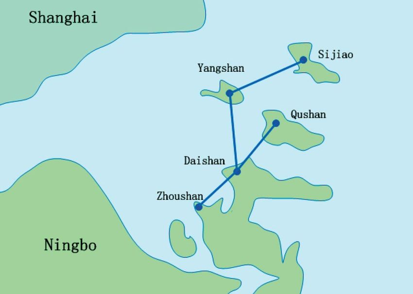
1.1 Zhoushan five-terminal HVDC grid [1]. . . . . . . . . . . . . . . . . . 2
1.2 (a) HB-SM’s and (b) FB-SM’s circuits and output voltage waveforms. 5
1.3 Fault-current path in an FM-MMC during a P2P fault. . . . . . . . . 6
1.4 Structure of HVDC systems: (a) point-to-point HVDC link, (b) MTDC
grid, and (c) meshed HVDC grid [2]. . . . . . . . . . . . . . . . . . . 6
1.5 Topology of a point-to-point HVDC link: (a) symmetric monopole
configuration, (b) asymmetric monopole configuration with ground
return, (c) asymmetric monopole configuration with metallic return,
(d) bipolar configuration with ground return, and (e) bipolar config-
uration with metallic return [3]. . . . . . . . . . . . . . . . . . . . . . 7
1.6 Grounding configuration for a symmetric monopole point-to-point HVDC
link: (a) with grounding branches between the transformer and MMC,
(b) with a resistor connecting to the neutral point of the transformer,
and (c) with series-connected resistors on the DC side [4]. . . . . . . . 9
2.1 Four-terminal meshed HVDC test grid. . . . . . . . . . . . . . . . . . 15
2.2 Equivalent MMC model right after a P2P fault [5]. . . . . . . . . . . 17
2.3 (a) Original and (b) equivalent circuits of an MMC right after a P2G
fault [6]. . . . . . . . . . . . . . . . . . . . . . . . . . . . . . . . . . . 18
2.4 MMC circuit during a positive P2G fault: (a) original circuit; (b)
steady-state circuit; and (c) fault circuit [6]. . . . . . . . . . . . . . . 19
2.5 (a) Circuit and (b) equivalent circuit for a single phase of an MMC [6]. 20
2.6 Equivalent model of the symmetric monopole test grid when a positive
P2G fault occurs on line 12 [6]. . . . . . . . . . . . . . . . . . . . . . 21
x2.7 Equivalent model of the symmetric monopole test grid when a P2P
fault occurs on line 12. . . . . . . . . . . . . . . . . . . . . . . . . . . 24
2.8 Equivalent model of the asymmetric monopole test grid with metallic
return when a positive P2G fault occurs on line 12. . . . . . . . . . . 25
2.9 Equivalent model of the bipole test grid with metallic return when a
positive P2M fault occurs on line 12. . . . . . . . . . . . . . . . . . . 27
2.10 (a) Faulty and (b) healthy line current derivatives during a P2P fault
on line 12 near MMC 1 in a symmetric monopole grid (rf = 0.01 Ω). 31
2.11 Initial current derivatives when a P2G fault occurs on different points
of line 12 in an symmetric monopole grid. . . . . . . . . . . . . . . . 32
2.12 Initial current derivatives when a P2P fault occurs on different points
of line 12 and line 24 in a bipole grid with metallic return. . . . . . . 32
3.1 Universal framework for relay jk in an HVDC system. . . . . . . . . 36
3.2 Operating principle of relay jk in a bipole grid with metallic return. . 38
3.3 Operating principle of relay jk in (a) a symmetric monopole grid, (b)
an asymmetric monopole grid with metallic return, and (c) a bipole
grid with ground return. . . . . . . . . . . . . . . . . . . . . . . . . . 39
3.4 Operating principle for relay jk in an asymmetric monopole grid with
ground return. . . . . . . . . . . . . . . . . . . . . . . . . . . . . . . 41
3.5 Matrices M4 , M4,1 , M4,2 , and M4,3 for b = 8. . . . . . . . . . . . . . 46
3.6 Current derivatives of each line during a P2P fault on line 12 near
MMC 1 (rf = 0.01 Ω). . . . . . . . . . . . . . . . . . . . . . . . . . . 50
3.7 Trip signals during a P2P fault on line 12 near MMC 1 (rf = 0.01 Ω). 51
3.8 Current derivatives on each line during a P2G fault on line 12 near
MMC 1 (rf = 500 Ω). . . . . . . . . . . . . . . . . . . . . . . . . . . . 52
3.9 Trip signals during a P2P fault on line 12 near MMC 1 (rf = 0.01 Ω). 52
3.10 Current derivatives of the fault line during a (a) P2P, (b) P2M, and
(c) P2G fault on line 12 near MMC 1 (rf = 0.01 Ω). . . . . . . . . . . 54
3.11 Current derivatives of (a) line 13, (b) line 14, (c) line 24, and (d)
line 34 during a P2P, P2G, and P2M fault on line 12 near MMC 1
(rf = 0.01 Ω). . . . . . . . . . . . . . . . . . . . . . . . . . . . . . . . 55
xi4.1 Voltage control of an MMC. . . . . . . . . . . . . . . . . . . . . . . . 59
4.2 Three types of four-terminal HVDC grids: (a) FFFF grid, (b) FHFH
grid, and (c) HHHH grid. . . . . . . . . . . . . . . . . . . . . . . . . . 61
4.3 Waveform during the restoration of the FFFF grid: (a) DC voltage
(fault cleared), (b)Vdc , 1 when the fault is cleared or not cleared, (c)
DC current (fault cleared), and (d) power (fault cleared). . . . . . . . 64
4.4 Comparison between the two restoration algorithms applied to the
FFFF grid: (a) DC voltages, (b) DC currents, and (c) power. . . . . . 65
4.5 Waveform at each terminal during the restoration of the FHFH grid:
(a) DC voltages, (b) DC currents, and (c) power. . . . . . . . . . . . 66
4.6 Waveform at each terminal during the restoration of the HHHH grid:
(a) DC voltages, (b) DC currents, and (c) power. . . . . . . . . . . . 66
xiiList of Tables
2.1 Converter and grid parameters . . . . . . . . . . . . . . . . . . . . . . 16
2.2 Matrix-form equations for all fault scenarios. . . . . . . . . . . . . . . 29
3.1 Characteristics of current derivatives in each grid topology and for
various fault scenarios . . . . . . . . . . . . . . . . . . . . . . . . . . 35
thx
3.2 Calculation method for threshold DIjk . . . . . . . . . . . . . . . . . 48
3.3 Thresholds for the symmetric monopole grid . . . . . . . . . . . . . . 49
3.4 Thresholds for the bipole grid with metallic return . . . . . . . . . . . 49
∗
4.1 Several pairs of (vout,HB ,vout,HB ) . . . . . . . . . . . . . . . . . . . . . 60
4.2 Parameters of the HVDC grid . . . . . . . . . . . . . . . . . . . . . . 62
4.3 Restoration sequence of the three HVDC grids . . . . . . . . . . . . . 65
xiiiNomenclature
i, v current and voltage vectors
0, 1, I all-zeros, all-ones, and identity matrices
A incidence matrix for an HVDC grid
R, L, E resistance, inductance, and elastance matrices
U(·), L(·) upper and lower bounds for a variable
g , c , l elements corresponding to the grounding branch, equivalent MMC
branch, and transmission line (the empty squares represent any vari-
ables)
p , n , m elements corresponding to the positive, negative, and metallic poles
0 , f elements corresponding to the pre-fault and post-fault scenarios
jk elements corresponding to line jk
j , f elements corresponding to terminal j and the fault point
pp , pg , pm elements corresponding to the pole-to-pole, pole-to-ground, and pole-
to-metallic fault scenarios
DIth the threshold for the current derivative-based relaying algorithm
rarm , larm arm resistance and inductance of an MMC
Vdc rated DC voltage of an MMC
Vm peak AC phase voltage
xivP2G pole-to-ground
P2M pole-to-metallic
P2P pole-to-pole
xvChapter 1
Introduction
1.1 HVDC grids
The global warming resulted from the extensive burning of fossil fuels has demon-
strate devastating impacts on the environment, wildlife, and humans, such as extreme
heat waves, biodiversity loss, and food crisis [7, 8]. As a response to the climate-
change threat, 194 states and the European Union have signed the Paris Agreement
by February 2021, which aims to limit the global temperature rise of this century well
below 2 degrees Celsius above pre-industrial levels [9]. This goal should be achieved
by obtaining net-zero emission of carbon dioxide (CO2 ) by 2050 [10], where zero-
carbon resources are expected to supply 76% of electricity globally [11]. Particularly,
as the main driver of this decarbonization process, wind and PV sources should grow
from 9% of the global electricity generation today to 56% by 2050 [11]. However,
the addition of renewable resources to the existing energy system to reduce the CO2
emission has resulted in various challenges to the security and stability of traditional
alternating current (AC) transmission systems due to the distributed and fluctuating
nature of renewable resources [5].
The high voltage direct current (HVDC) technology has significant potential for
resolving the security and stability issues of the AC power systems integrated with
large amounts of renewable resources because HVDC systems offer better control on
the power transmission compared to traditional AC systems [2, 12]. Furthermore,
HVDC lines can connect two asynchronous power systems and serve as a boundary
in case of a cascading failure. HVDC systems also offer a lower power loss for long-
distance power transmission between load centers and remote renewable resources
1[13]. All of the benefits of HVDC transmissions have resulted in a boost in the
HVDC market. According to [14, 15], the global HVDC converter station market is
expected to grow from USD 7.9 billion in 2017 to USD 15.74 billion by 2026, with
an average annual growth rate of 7.96%.
By 2020, there have been more than 200 HVDC projects operating or being
constructed all over the world [16]. These HVDC systems vary in topology, converter
type, grounding configuration, and grid configuration. For example, the world’s first
commercial HVDC link, Gotland 1, was operated in 1954 and is a point-to-point
asymmetric monopole grid based on the mercury arc valve using the sea for the
return current [17]. With the development of HVDC technology, in recent HVDC
projects, the state-of-art converters, environment-friendly grounding options, and
more flexible configurations are used to increase the controllability, flexibility, and
DC voltage level. For example, the Zhoushan five-terminal HVDC grid operated in
2014 is a bipolar grid using the modular multilevel converter (MMC) at each station
[18], Fig. 1.1. Compared to Gotland 1, the Zhoushan HVDC grid has a higher
degree of controllability on the DC voltage [19] and more redundancy in case of the
loss of a transmission pole [20]. The different topology, type of converters, grounding
configuration, and grid configuration of HVDC systems will result in different fault
responses, the analysis of which has significant importance to HVDC protection
design.
Figure 1.1: Zhoushan five-terminal HVDC grid [1].
21.1.1 Converters of HVDC Systems
There are three main technologies for HVDC converters, the line commuted converter
(LCC), two-level and three-level voltage source converters (VSCs), and the modular
multilevel converter (MMC) [21, 22]. For the sake of simplicity, VSC in the remaining
part of this thesis corresponds to a two-level or three-level converter.
The LCC, also known as a current source converter, uses semi-controlled thyris-
tors as switches [21]. On the contrary, the VSC, which employs fully-controlled
insulated-gate bipolar transistors (IGBTs) for AC-DC conversion, has a higher de-
gree of controllability than the LCC. The VSC is able to [21, 23]
• be connected with a weak AC grid,
• perform black start,
• control active power and reactive power separately, and thus requires no addi-
tional reactive power compensation, and
• achieve a bi-directional power transmission.
However, a VSC should operate at a high frequency to reduce harmonics in the DC
voltage waveform, which will result in high switching losses. Furthermore, the voltage
level of a VSC is restricted by the voltage rating of IGBTs. In order to overcome
the two main disadvantages of the VSC, the technology of MMC was developed [23].
An MMC consists of six arms, where each arm connects an AC phase to a DC pole.
Multiple submodules (SMs) are connected in series and controlled separately in each
arm of an MMC. The voltage level of an MMC can be easily increased by increasing
the number of SMs in each arm. Meanwhile, the switching frequency of each IGBT
in an SM is around the AC frequency. Compared to the VSC, the MMC [22, 24]
• has lower switching losses,
• has a lower requirement for IGBT’s voltage rating,
• does not require the DC-link capacitor,
• can be modularly designed, and
• can generate the DC voltage with fewer harmonics.
3Being benefited by so many advantages, the MMC has become the most favorable
type of converter for HVDC systems [25]. This thesis will only focus on HVDC
systems based on MMCs.
Each SM is a basic AC-DC conversion circuit consisting of IGBTs, freewheeling-
diodes, and DC capacitors. Different types of SMs have various operating principles
and fault ride-through characteristics. This subsection will introduce two basic SMs,
the half-bridge (HB)-SM and the full-bridge (FB)-SM.
An HB-SM consists of two IGBTs with freewheeling-diodes (S1 and S1 ) and a
DC capacitor (C) [22], Fig. 1.2(a). During the normal operation, the capacitor
voltage vc is regulated around a constant value NVSMdc
, where Vdc is the rated output
DC voltage of the MMC, and NSM is the number of SMs in each arm of the MMC.
An HB-SM can output a two-level voltage, vc or 0. If S1 is in the on-state (S1 = 1),
the output voltage vH is vc ; if S1 is in the off-state (S1 = 0), vH = 0. Since an
HB-SM can only generate a monopole output voltage, Vdc of an HB-MMC cannot
be smaller than the peak AC phase voltage [26]. If a DC fault occurs, the MMC will
be blocked—all IGBTs in the MMC are switched to the off-state—to protect each
device from being damaged by the large DC fault current. However, the HB-SM does
not have the fault-current interrupting capability. Even though the each HB-SM is
blocked during the fault, the fault current can still flow through the freewheeling-
diodes until the fault disappears, the MMC is disconnected from the fault, or the AC
grid is disconnected from the MMC. As a compensation for HB-MMC’s incapability
of interrupting the fault current, DC circuit breakers (DCCBs) or AC circuit breakers
(ACCBs) should be installed on the DC side or the AC side, respectively.
An FB-SM consists of four IGBTs with freewheeling-diodes (S1 , S1 , S2 , and S2 )
and a capacitor (C), Fig. 1.2(b). Each FB-SM can output a three-level voltage, vc ,
−vc , or 0. If S1 and S2 are both 1, vF = vc ; conversely, if S1 and S2 are both 0,
vF = −vc ; if S1 and S2 are of different values (S1 = 1 and S2 = 0 or S1 = 0 and
S2 = 1), vF = 0. Since an FB-SM can generate a bipolar output voltage, the Vdc of a
FB-MMC can be smaller than the peak AC phase voltage [26]. This characteristic is
useful for a FB-MMC to raise the DC grid voltage smoothly during the restoration
process. If a FB-MMC is blocked during a fault, the four IGBTs in each FB-SM
will all be switched to the off-state so that the fault current cannot flow through
them. In this case, the DC fault current will be interrupted by the FB-MMC when
each FB-SM capacitors are fully charged. Fig. 1.3 shows the fault-current path in
an FB-MMC, whose each arm contains only one FB-SM for the sake of simplicity
and AC side is ∆-connected. For example, after the occurrence of a pole-to-pole
(P2P) fault in an HVDC grid, if the phase A-to-C voltage reaches its peak, the fault
4-
0
(a)
- 0
(b)
Figure 1.2: (a) HB-SM’s and (b) FB-SM’s circuits and output voltage waveforms.
current will flow from phase A, flow through the diodes in the SMs on the upper arm
connected to phase A, charge the capacitors in these SMs, flow from the positive pole
to the negative pole through the fault point, flow through the SMs on the lower arm
connected to phase C, charge corresponding capacitors, and return to phase C, Fig.
1.3. During the process that the fault current charges SM capacitors, the capacitor
voltages are rising. When the sum of SM-capacitor voltages of an upper arm and a
lower arm rises to the peak phase-to-phase AC voltage Vm , the AC side will not feed
any fault current to the HVDC grid. As a result, the fault current is interrupted by
the blocked FB-MMC. Since FB-MMCs can interrupt fault currents, neither DCCBs
nor ACCBs are required to be installed around FB-MMCs in a point-to-point HVDC
link.
1.1.2 HVDC System Structure
Based on structure, HVDC systems can be classified into point-to-point HVDC links,
multi-terminal HVDC (MTDC) grids, and meshed HVDC grids [2]. HVDC systems
in these three structures are shown in Fig. 1.4.
The point-to-point HVDC link can be embedded in an AC grid for transferring
bulk electric power over long distances. Both an MTDC grid and a meshed HVDC
5- - -
A
B
C
- - -
Figure 1.3: Fault-current path in an FM-MMC during a P2P fault.
~
=
~ ~
~ ~ = =
~ ~ = =
= = ~ ~
~ = =
=
(a) (b) (c)
Figure 1.4: Structure of HVDC systems: (a) point-to-point HVDC link, (b) MTDC
grid, and (c) meshed HVDC grid [2].
grid contain multiple converter terminals. The major difference between these two
grids is that the meshed HVDC grid contains at least one loop while an MTDC grid
does not [2]. Being benefited by the transmission loop, a meshed HVDC grid can
function normally even when a transmission line in the loop is lost. However, a more
complex grid structure requires more advanced converters. For example, a meshed
HVDC grid can only use VSCs or MMCs, while an MTDC grid can use LCCs, VSCs,
6or MMCs. Compared to traditional HVAC grids, meshed HVDC grids and MTDC
grids demonstrate an improved performance in reducing grid congestion, providing
increased system stability, and enabling the interconnection of asynchronous power
resources [2].
1.1.3 Topology and Grounding Configurations of HVDC Sys-
tems
HVDC systems can be formed in various topologies such as symmetric monopole,
asymmetric monopole with ground or metallic return, and bipole with ground or
metallic return [20], Fig. 1.5. This subsection will introduce the above five topologies
with their corresponding grounding configurations briefly.
~ ~ ~ ~
= = = =
(a) (b)
~ ~
~ ~ = =
= =
~ ~
= =
(d)
(c)
~ ~
= =
~ ~
= =
(e)
Figure 1.5: Topology of a point-to-point HVDC link: (a) symmetric monopole config-
uration, (b) asymmetric monopole configuration with ground return, (c) asymmetric
monopole configuration with metallic return, (d) bipolar configuration with ground
return, and (e) bipolar configuration with metallic return [3].
A symmetric monopole system contains one MMC at each terminal and employs
7two transmission lines corresponding to two poles for a transmission path, where
each line requires full insulation. If a P2P fault occurs on the transmission line,
the power transmission in this system will be interrupted until the fault is cleared.
If a pole-to-ground fault occurs, the fault response of the system varies depending
on the grounding configuration on the AC side [4], Fig. 1.6. In the first ground-
ing configuration, the transformer on the AC side is Y-∆ connected to the MMC,
and grounding branches are installed between the transformer and the MMC, Fig.
1.6(a). If a P2G fault occurs, the grounding branches will supply the unbalanced
fault current. In order to restrict the magnitude and rising speed of fault current,
inductors and resister in grounding branches should be large, e.g., Lg = 3 H and
Rg = 1000 Ω [6]. In the second grounding configuration, the transformer is ∆-Y con-
nected to the MMC, and a large grounding resister is connected to the neutral point
of the transformer, Fig. 1.6(b). The flowing path of fault current in this configura-
tion during a P2G fault is similar to that in the first configuration, except the fault
current in this configuration will flow through the secondary side of the transformer.
From the transformer protection perspective, this configuration can only be used in
low voltage systems. In the third configuration, the transformer is ∆-Y connected to
the MMC, and two series-connected resistors are installed on the DC side with the
neutral point grounded, Fig. 1.6(c). These two resistors may result in DC voltage
unbalance and will increase the power loss. Consequently, this configuration cannot
be used in a high-voltage grid. Among the three configurations, the first grounding
configuration is the most reliable and is used in many existing HVDC systems, e.g.,
the Trans Bay Cable in the USA. As a result, in this thesis, the symmetric monopole
grid has the first grounding configuration.
An asymmetric monopole system only uses one pole for power transmission, and
that pole is preferred to be the negative pole to reduce corona effects [27]. The return
current can flow through the ground or metallic conductor. If the ground return is
used, each terminal should be low-impedance grounded to reduce the power loss [20].
In this configuration, continuous return current will flow through the ground along
the transmission path, which requires specific permission [3]. Specifically, sea can also
be used for the return current, e.g., Gotland 1 HVDC line [17]. If the metallic return
is used, only one terminal should be low-impedance grounded, and other terminals
can be high-resistance grounded or ungrounded [20].
A bipolar system contains two MMCs at each terminal, where each MMC con-
nects a pole and the neutral point, which can be low- or high-impedance grounded.
The grid can use ground return or metallic return [20]. If the ground return is used,
all terminals should be low-impedance or high-impedance grounded. In this config-
8Grounding
branches
(a)
(b)
(c)
Figure 1.6: Grounding configuration for a symmetric monopole point-to-point HVDC
link: (a) with grounding branches between the transformer and MMC, (b) with
a resistor connecting to the neutral point of the transformer, and (c) with series-
connected resistors on the DC side [4].
9uration, no continuous ground current will flow through the transmission path, but
the permission for temporary operating with ground current is still required [3]. If
the metallic return is used, at least one terminal should be grounded, and other ter-
minals can be high-impedance grounded or ungrounded. The bipolar grid has a 50%
redundancy; therefore, if a P2G or pole-to-metallic (P2M) fault occurs on the grid,
the power transmission on the healthy pole—50% of the rated grid capacity—will
not be interrupted.
1.2 Statement of the Problem and Thesis Objec-
tives
Although extensive research has been conducted on the protection of HVDC systems,
a universal protection scheme for HVDC systems in various forms has not been
proposed. The objective of this thesis is to develop a universal protection scheme
that is suitable for HVDC systems in various forms. The variety of system forms
includes three aspects:
• structure of the system, i.e., point-to-point, MTDC, or meshed HVDC,
• type of MMCs in the system, i.e., only FB-MMCs, only HB-MMCs, or both
FB- and HB-MMCs, and
• system topology and grounding configuration, i.e., symmetric monopole, asym-
metric monopole with ground or metallic return, or bipole with ground or
metallic return.
A universal protection scheme for HVDC systems contains two parts: a universal
relaying scheme and a universal restoration algorithm to quickly restore the system
with low voltage oscillations and limited inrush currents. The developed relaying
scheme only uses the locally measured current derivatives to detect internal faults,
and the relay settings are calculated based on differential equations of the system
after fault occurrence instead of being obtained by extensive time-consuming elec-
tromagnetic transient (EMT) simulations.
In order to fulfill the objective of this thesis, the following methodology is used:
• Each component in an MMC-based HVDC system is linearized and an equiv-
alent circuit of an MMC-based HVDC system right after a DC fault is built,
10• A matrix-form differential equation that can calculate the current derivative of
each line right after a DC fault is developed (for each grid form and each fault
scenario, a matrix-form equation is developed),
• A method that uses the calculated post-fault current derivative of each line to
determine the setting of each relay in an HVDC system is developed,
• A linear control block for HB-MMCs to raise the grid DC voltage stably during
the restoration process is designed, and
• Time-domain simulations in PSCAD/EMTDC that can demonstrate the feasi-
bility of the relaying scheme and restoration algorithm are performed. Various
grid configurations and fault scenarios are investigated in PSCAD/EMTDC.
1.3 Thesis Layout
The rest of this thesis is organized as follows:
• Chapter 2 presents an approach to build the equivalent circuits and construct
the matrix-form differential equations for post-fault MMC-HVDC grids in var-
ious topologies under various fault scenarios. In the simulation section, the
matrix-form differential equation is used to calculate the fault current in an
HVDC grid right after a DC fault. The accuracy of the differential equation is
discussed in various grid topologies under various fault scenarios.
• Chapter 3 presents a universal relaying scheme, specific relaying algorithms
corresponding to various grid topologies, and a new method that uses differen-
tial equations to calculate the relay settings. In the simulation section, various
types of DC faults are employed to grids in various topologies to evaluate the
performance of the developed relaying algorithms and the calculated relaying
settings.
• Chapter 4 analyzes the voltage-control and power-control abilities of FB- and
HB-MMCs during the restoration process and presents a universal algorithm
for the restoration of various types of HVDC grids, which may even contain
different types of MMCs with and without fault blocking capability. A voltage-
control block is designed for HB-MMCs to stabilize the rise of the DC voltage
during restoration when the HB-MMC controls the DC voltage in the HVDC
11grid. In the simulation section, the performances of the developed restoration
algorithm is evaluated.
• Chapter 5 presents the contributions and conclusions of this thesis and points
out the directions for future work.
12Chapter 2
Fault-Current Calculation for
HVDC Systems
2.1 Introduction
The design of a relaying algorithm for HVDC grids requires comprehensive under-
standing of the fault transient, which can be obtained by performing electromagnetic
transient (EMT) simulations, frequency-domain analysis, or time-domain analysis on
the equivalent models of HVDC grids. In the literature, various equivalent models of
HVDC components are developed to achieve the fault-transient analysis in various
levels of details.
An MMC can be built as a detailed model [22, 28], a continuous model [29], or a
RLC branch [5, 30, 31]. The detailed MMC model is constructed with the the highest
fidelity, where each SM and non-linear semiconductor device is individually modeled
and controlled. For some highly detailed models, the temperature effect on semicon-
ductors is even simulated. The detailed model enables the analysis in the level of
devices, such as the behavior of an individual SM during a transient. However, the
extensive appearance of nonlinear devices in the detailed model requires significant
calculation resources and comprises the model’s calculation efficiency. If only the
analysis in the grid level is required, the MMC can be represent by a continuous
model [29], which consists of a controlled voltage source with a few semiconductor
switches. The continuous model is of high accuracy during the steady state, fault
transient, and operation transient. Meanwhile, the simulation efficiency of the con-
tinuous model is significantly higher than that of the detailed model. If the analysis
13only focuses on the period right after the fault (tens of milliseconds), a RLC branch
with [30, 31] or without a controlled current source [5, 6] can be used to represent
an MMC. The equivalent RLC branch significantly simplifies the MMC and enables
the mathematical expression of the fault current right after a fault.
An transmission line can be represented by the frequency dependent (FD) model,
the lumped Π model, or a RL branch. In the FD model, the line resistance, induc-
tance, and capacitance are distributed along the transmission line, and the traveling-
wave dispersion resulted from the different propagation speeds of traveling-waves
with different frequencies is considered. The FD model is excellent in describing the
traveling wave phenomenons during the transient, such as the propagation of fault
current and the over voltage resulted from the reflected traveling waves between ter-
minals. However, it is hard to use the FD model to analyze the fault transients in
HVDC grids other than by using simulation tools. The lumped Π model, which rep-
resents a transmission line with a resister, an inductor, and two capacitors, enables a
mathematical approach to describe the HVDC grid with impedance or conductance
matrix. If a transmission line has small capacitance, e.g., an overhead line, this line
can be further simplified as a RL model. Both the lumped Π model and the RL
model provide the approach to mathematically express the fault current right after
the fault occurrence with acceptable accuracy.
This chapter presents a set of matrix-form differential equations to calculate the
fault current in HVDC grids right after a DC fault. The matrix-form differential
equations can be easily built and are suitable for:
• various grid topologies, e.g., symmetric monopole, asymmetric monopole with
ground or metallic return, and bipole with ground or metallic return;
• various fault scenarios, e.g., P2P, P2G, and pole-to-metallic (P2M) faults;
• grids with different types of MMCs, e.g., a grid with both FB-MMCs and
HB-MMCs.
Section 2.2 introduces the test grid. Section 2.3 presents the matrix-form equations
for various grid topologies and fault scenarios. Section 2.4 evaluates the accuracy of
the developed calculation methods.
14Fault points
FB-MMC 1 HB-MMC 2
= line 12 =
~ (100 km) ~
line 13 line 24
(200 km) (150 km)
HB-MMC 3 line 14
FB-MMC 4
(200 km)
= =
~ ~
line 34
(100 km)
Figure 2.1: Four-terminal meshed HVDC test grid.
2.2 Test Grids
Five four-terminal meshed HVDC grids in different configurations—symmetric monopole,
asymmetric monopole with ground or metallic return, and bipole with ground or
metallic return—are tested in this chapter, Fig. 2.1. For each configuration, FB-
MMCs are installed at terminals 1 and 4, and HB-MMCs are installed at terminals
2 and 3. The rated DC voltage of each MMC station is Vdc = 640 kV, i.e., the rated
P2P voltage of the bipole grid is 2Vdc .
For each configuration, the MMC is connected to the AC grid through a ∆-Y
connected transformer, where ∆ and Y are on MMC and AC sides, respectively
[6]. For the symmetric monopole grid, each MMC is connected with grounding
branches—three Y-connected inductors in series with a resistor—on the AC side and
un-grounded on the DC side [4], Fig. 2.2. The asymmetric monopole and bipole grids
have no grounding branch on the AC side and are low-impedance (10 Ω) grounded on
the DC side. The asymmetric monopole grid uses the negative pole for transmission.
Transmission lines in test grids are overhead lines (OHLs), which are represented
by RL branches [30] to simplify the calculation of fault currents. At both ends of a
line, terminal inductors are implemented to limit the rising speed of the fault current
[32]. Between each MMC and a terminal inductor, a hybrid DCCB is implemented.
The hybrid DCCB model is presented by [33], which will open within 2 ms after
receiving a trip signal generated by the relay. Between the two terminal inductors
on each line, eleven fault points are equally distributed. These fault points will be
used in Section 2.4.3. For the sake of simplicity, these fault points are only shown on
line 12 in Fig. 2.1. The grid and converter parameters are shown in Table 2.1 [6].
15Table 2.1: Converter and grid parameters
Items Values
Converter stations
AC grid voltage 400 kV
Nominal ratio of transformer 400 kV/380 kV
Transformer leakage inductance (uk ) 0.15 p.u.
Grounding inductance (lac ) 3H
Grounding resistance (rac ) 1000 Ω
Dc grid rated voltage (Vdc ) 640 kV
Sub-module (SM) capacitance (cSM ) 10000 µF
IGBT and diode on-state resistance (rON ) 5 mΩ
Arm inductance (larm ) 20 mH
Arm resistance (rarm ) 0Ω
Number of SMs per arm (NSM ) 76
DC overhead lines
Resistance per unit length 0.014 Ω/km
Inductance per unit length 0.82 mH/km
Terminal inductance (lt ) 50 mH
Control mode
FB-MMC 1 Vdc =640 kV
HB-MMC 2 P =-900 MW
HB-MMC 3 P =-900 MW
FB-MMC 4 P =950 MW
2.3 Calculation of Fault-Current Derivatives
This section introduces a new methods to calculate the DC current right after a DC
fault occurs in a multi-terminal HVDC grid. All of the grid topologies and fault
scenarios are covered by the calculation methods. Namely, a P2G or P2P fault in a
symmetric monopole grid, a P2G fault in an asymmetric monopole grid with ground
return, a P2G or P2M fault in an asymmetric monopole grid with metallic return,
a P2G or P2P fault in a bipole grid with ground return, and a P2G, P2M, or P2P
fault in a bipole grid with metallic return are studied in this section. An advantage
of the calculation methods is that the differential equations used for the calculation
are all in the similar matrix forms, and these matrices can be easily built or modified
once an HVDC grid is expanded or reconstructed
16This section will introduce the calculation method for four typical fault scenarios—
P2G and P2P faults in a symmetric monopole grid, a P2G fault in an asymmetric
monopole grid with metallic return, and a P2M fault in a bipole grid with metallic
return—and a uniform matrix-form equation with a table where matrices for all fault
scenarios are listed. The equivalent MMC models are introduced in 2.3.1, and the
current calculation method for the four fault scenarios is introduced in 2.3.2-2.3.6.
2.3.1 Equivalent MMCs right after a DC Fault
Right after a P2P fault, an MMC can be represented by an RLC branch [5], Fig.
2.2. After the fault occurrence and before the operation of the protection system
(less than 10 ms), SM capacitors discharge rapidly and lead to large fault currents.
Comparatively, currents from the AC side are small, so the AC side is not considered
in this equivalent MMC model [5, 34]. Parameters of the equivalent MMC model are
or
+
FB-SM HB-SM
-
Figure 2.2: Equivalent MMC model right after a P2P fault [5].
expressed as (2.1) [5],
2(rjarm + NSM N2sw rON )
rjc = , (2.1a)
3
2ljarm
ljc = , (2.1b)
3
6cSMj
ccj = , (2.1c)
NSM
17where rjarm and ljarm are arm resistance and inductance of MMC j, respectively; NSM
is the number of SMs in each arm; Nsw is the number of IGBTs in an SM, e.g., Nsw
is 2 in a HB-SM and is 4 in an FB-SM; rON is the on-state resistance of an IGBT
or diode; cSM
j is the SM capacitance of MMC j; and rjc , ljc , and ccj are the equivalent
resistance, inductance, and capacitance of MMC j, respectively.
Right after a P2G fault, an MMC can be represented by the aforementioned RLC
branch with two equivalent grounding branches as shown in Fig. 2.3(b), the proof of
which is expressed below [6].
+
-
(a) (b)
Figure 2.3: (a) Original and (b) equivalent circuits of an MMC right after a P2G
fault [6].
According to the superposition principle, an MMC terminal during a P2G fault,
Fig. 2.4(a), can be decomposed into a steady-state circuit, Fig. 2.4(c), and a fault
circuit, Fig. 2.4(c). Since the ∆-connected transformer on the AC side cannot provide
the unbalanced P2G fault current, the steady-state circuit can be neglected during
the P2G-fault analysis.
Fig. 2.5(a) shows a single phase of the circuit in Fig. 2.4(c). Since the grounding
impedance is much larger than the upper and lower arm impedances (Zjg
Zjp and
Zjn ), the equivalent ∆-connected circuit in Fig. 2.5(b) can be approximated as (2.2)
by employing the Y-∆ transform.
18(a)
+ -
- +
(b) (c)
Figure 2.4: MMC circuit during a positive P2G fault: (a) original circuit; (b) steady-
state circuit; and (c) fault circuit [6].
Zjg Zjp
Zjpg = Zjg + Zjp + ≈ 2Zjg = j2ωljac + 6rjac , (2.2a)
Zjn
Zjg Zjn
Zjng = Zjg + Zjn + ≈ 2Zjg = j2ωljac + 6rjac , (2.2b)
Zjp
Zjp Zjn 1
Zjpn = Zjp + Zjn + ≈ Zjp + Zjn = −j + j2ωljarm + 2rjarm , (2.2c)
Zjg ωCi
where Zjpg , Zjng , and Zjpn are the equivalent impedances of the ∆-connected circuit
19(a) (b)
Figure 2.5: (a) Circuit and (b) equivalent circuit for a single phase of an MMC [6].
in Fig. 2.5(b). cpn
j can be calculated based on the energy balance principle [35, 36]:
1 cpn V 2 = 2N × 1 cSM V 2
SM 2 SM
2 j dc 2 SM
⇒ cpn
j = c . (2.3)
NSM
Vdc = NSM VSM
The equivalent MMC during a P2G fault can be obtained by connecting three of the
circuits shown in Fig. 2.5(b) in parallel. As a result, the parameters of the equivalent
grounding branch are expressed as (2.4),
2ljac
ljg = , (2.4a)
3
ac
6rj
rjg = = 2rjac , (2.4b)
3
where rjg and ljg are the equivalent resistance and inductance of the grounding
branches for MMC j, respectively.
2.3.2 P2G Fault in the Symmetric Monopole Grid
Fig. 2.6 shows the equivalent test grid when a positive P2G fault occurs on line
12. Branch currents ipjk and injk are the positive and negative pole currents flowing
from MMC j to MMC k, respectively. Branch currents of faulty lines are ip1f and
ipf 2 , where f denotes the fault point. The capacitor current icj is flowing from the
20negative pole of MMC j to its positive pole. Ground currents ipj and inj are flowing
from the ground to positive and negative poles of MMC j, respectively. The voltage
across ccj is vjc . Bold variables ip , in , ic , and v c represent column vectors of ipjk , injk , icj ,
and vjc , respectively. Specifically, two faulty line currents form the last two elements
of the current vector, i.e., ip (5) = ip1f and ip (6) = ipf 2 for the test grid.
MMC 1 MMC 2
MMC 3 MMC 4
Figure 2.6: Equivalent model of the symmetric monopole test grid when a positive
P2G fault occurs on line 12 [6].
For each current in ip , in , and ic , a differential equation can be formed by em-
ploying KVL to the electrical path that the current passes. For example, equations
for ip34 , ip1f , in12 , and ic1 is expressed in (2.5a), (2.5b), (2.5c), and (2.5d), respectively.
dip3 dip dip
0 = r3g ip3 + r34 ip34 − r4g ip4 + l3g + l34 34 − l4g 4 , (2.5a)
dt dt dt
p p
di di 1f
0 = r1g ip1 + r1f ip1f + rf if + l1g 1 + l1f , (2.5b)
dt dt
din din din
0 = r1g in1 + r12 in12 − r2g in2 + l1g 1 + l12 12 − l2g 2 , (2.5c)
dt dt dt
n c p
c g n c c g p g di1 c di1 g di1
v1 = r1 i1 + r1 i1 − r1 i1 + l1 + l1 − l1 . (2.5d)
dt dt dt
Each ground current can be replaced by the sum of certain currents in ip , in , and ic .
For example, ip1 = ip1f + ip13 + ip14 − ic1 , and in1 = in12 + in13 + in14 + ic1 . Replacing ground
21currents in (2.5a-2.5d) with currents in ip , in , and ic yields
0 = − r3g ip13 + r4g ip14 + r4g ip24 + (r34 + r3g + r4g )ip34 − r3g ic3 + r4g ic4
dip13 dip dip dip dic dic (2.6a)
− l3g + l4g 14 + l4g 24 + (l34 + l3g + l4g ) 34 − l3g 3 + l4g 4 ,
dt dt dt dt dt dt
0 =(r1f + r1g + rf )ip1f − rf ipf 2 + r1g ip13 + r1g ip14 − r1g ic1
dip1f dip13 dip dic (2.6b)
+ (l1f + l1g ) + l1g + l1g 14 − l1g 1 ,
dt dt dt dt
0 =r1g in13 + r1g in14 − r2g in24 + (r12 + r1g + r2g )in12 + r1g ic1 − r2g ic2
din din din din dic dic (2.6c)
+ l1g 13 + l1g 14 − l2g 24 + (l12 + l1g + l2g ) 12 + l1g 1 − l2g 2 ,
dt dt dt dt dt dt
v1c = − r1g (ip1f + ip13 + ip14 − in12 − in13 − in14 ) + (r1c + 2r1g )ic1
d p dic (2.6d)
− l1g (i1f + ip13 + ip14 − in12 − in13 − in14 ) + (l1c + 2l1g ) 1 .
dt dt
2.3.2.1 The matrix-form representation of currents and voltages rela-
tionship
There are 2b+N +1 currents in ip , in , and ic in total, where N is the number of MMC
terminals, and b is the number of positive pole lines before the fault occurrence. The
equations for all currents can be expressed in the matrix form,
di
Apg · v c = Rpg · i + Lpg · , (2.7)
dt
where Apg = [0N,2b+1 , IN ]> , i = [ip> , in> , ic> ]> , and IN is a N × N identity matrix.
The first b − 1 rows in (2.7) are in the form similar to (2.6a), and they correspond to
the positive healthy pole currents. Likewise, the bth to (b+1)th , (b+2)th to (2b+1)th ,
and (2b + 2)th to (2b + N + 1)th rows are in the forms similar to (2.6b), (2.6c), and
(2.6d), respectively.
Rpg and Lpg are (2b + N + 1) × (2b + N + 1) resistance and inductance matrices,
respectively. Rpg is expressed as
Af (Rg + Rf )A> l
−Af Rg
f + Rf 0b+1,b
Rpg = 0b,b+1 A0 Rg A> l
0 + R0 A0 Rg , (2.8)
−Rg > A> f
g> >
R A0 Rc + 2Rg
where A0 is the incidence matrix for the pre-fault grid which has a row for each
transmission line and a column for each terminal [37]. Af is the incidence matrix for
the post-fault grid, which is formed by 1) splitting the row in A0 corresponding to
the faulty line into two rows that contain a non-zero element, and 2) moving these
22two rows to the bottom of A0 . For example, A0 and Af for the test grid during a
P2G fault on line 12 are shown in (2.9).
1 0 −1 0
1 −1 0 0 1 0 0 −1
1 0 −1 0
0 1 0 −1
1
A0 = 0 0 −1, Af = . (2.9)
0 0 1 −1
0 1 0 −1
1
0 0 0
0 0 1 −1
0 −1 0 0
Rg , Rc , Rl0 , and Rlf are diagonal matrices with ground resistances, MMC equivalent
resistances, line resistances of the pre-fault and post-fault grids on diagonals, respec-
tively. The sequences of line resistances in Rl0 and Rlf correspond to the sequences
of lines in A0 and Af , respectively. Rf is the fault resistance matrix. For example,
these matrices for the test grid are
Rg = diag(r1g , r2g , r3g , r4g ), (2.10a)
Rc = diag(r1c , r2c , r3c , r4c ), (2.10b)
Rl0 = diag(r12 , r13 , r14 , r24 , r34 ), (2.10c)
Rlf = diag(r13 , r14 , r24 , r34 , r1f , rf 2 ), (2.10d)
f
R = rf · 14,4 , (2.10e)
where 14,4 is a 4 × 4 all-ones matrix, and the diagonal function diag(·) is defined in
[38].
The structure of Lpg is the same as Rpg , except all R and r in Rpg are replaced
by L and l, respectively. Generally, Lf is a zero matrix.
The matrix form equation for all capacitor voltages is expressed as
dv
= −Ec · A>
pg · i, (2.11)
dt
where the elastance matrix Ec is a diagonal matrix with the reciprocal of each equiv-
alent MMC’s capacitance as the element,
Ec = diag(1/cc1 , · · · , 1/ccj , · · · , 1/ccN . (2.12)
Combining (2.7) and (2.11) yields the matrix-form equation for the P2G fault
scenario, −1 −1
d i −Lpg · Rpg Lpg · Apg i
= · , (2.13)
dt v Epg 0N,N v
where Epg = −Ec · A>
pg .
232.3.3 P2P Fault in the Symmetric Monopole Grid
Fig. 2.7 shows the equivalent model of the symmetric monopole test grid when a
P2P fault occurs on line 12. The matrix-form equation for a P2P fault scenario is
expressed as (2.14) [5].
MMC 1 MMC 2
MMC 3 MMC 4
Figure 2.7: Equivalent model of the symmetric monopole test grid when a P2P fault
occurs on line 12.
d ip
−1 p
−Lpp · Rpp L−1
pp · App i
= · c . (2.14)
dt v c Epp 0N,N v
Rpp and Lpp are (b + 1) × (b + 1) resistance and inductance matrices, respectively.
Epp is a N × (b + 1) elastance matrix.
App = Af , (2.15a)
Rpp = Af (R + R )A>
c
f
f
+ 2Rlf , (2.15b)
c > l
Lpp = Af L Af + 2Lf , (2.15c)
Epp = −Ec · A>
pp . (2.15d)
Af , Rc , Rf , Rlf , Lc , Llf , and Ec are the same as expressed previously.
2.3.4 P2G fault in the Asymmetric Monopole Grid with
Metallic Return
The equivalent circuit when a negative P2G fault occurs on line 12 in the asymmetric
monopole test grid with metallic return is shown in Fig. 2.8. Since each MMC
24MMC 1 MMC 2
MMC 3 MMC 4
Figure 2.8: Equivalent model of the asymmetric monopole test grid with metallic
return when a positive P2G fault occurs on line 12.
connects the neutral point with the negative pole, the voltage of the equivalent
capacitor of MMC j is denoted as vjcn , the positive direction of which is from the
neutral point to the negative pole, Fig. 2.8. The voltage vector, MMC current vector,
MMC resistance matrix, MMC inductance matrix, and MMC conductance matrix
are denoted as v cn , icn , Rcn , Lcn , and Ecn , respectively. The vector im consists of
each current on the metallic return line. The matrices Rm m
0 and L0 are similar to
l l m m
R0 and L0 , respectively, except that R0 and L0 correspond to the metallic return
lines. For example, im and Rm 0 for the asymmetric monopole test grid with metallic
return are expressed as
m m m m >
im = [im
12 , i13 , i14 , i24 , i34 ] , (2.16a)
Rm
0 = m m m m m
diag(r12 , r13 , r14 , r24 , r34 ). (2.16b)
Rg and Lg are still diagonal matrices consisting of the grounding resistance and
grounding inductance at each terminal, respectively. If MMC j is ungrounded, rjg
and ljg should be set at a very large value, e.g., 100 times larger than the maximum
line resistance and inductance, respectively.
The matrix-form equation for this scenario is express as
−1
−L−1
d i −Lpg · Rpg pg · Apg i
= · cn , (2.17)
dt v cn −Epg 0N,N v
25where
i = [in> , im> ]> , (2.18a)
Apg = [A> >
f , 0N,b ] , (2.18b)
Af (Rcn + Rg f
)A> Rlf Af R A>
g
+R f + 0
Rpg = , (2.18c)
A 0 Rg A >
f A0 Rg A> m
0 + R0
Af (Lcn + Lg )A> l
Af Lg A>
f + Lf 0
Lpg = g > m , (2.18d)
A0 L Af A0 Lg A>
0 + L0
Epg = −Ecn · A>
pg . (2.18e)
If the test grid is low-resistance grounded at one MMC terminal and ungrounded
at other terminals, the earth current during normal operation will be small, but
P2G faults far away from the grounding terminal can be hardly detected. If one
terminal is low-resistance grounded and others are high-resistance grounded, the
earth current during normal operation will be small, and P2G faults far away from
the low-resistance grounded terminal can be detected easily.
2.3.5 P2M fault in the Bipole Grid with Metallic Return
The equivalent circuit when a fault occurs on line 12 in the bipole test grid with
metallic return is shown in Fig. 2.9. In this fault scenario, the P2M fault branch is
considered as a virtual MMC with an equivalent resistance of rf , zero inductance, no
capacitance, ground resistance of rfg , and ground inductance of lfg , where rfg and lfg
are arbitrary large values that are 100 times larger than the maximum line resistance
and inductance, respectively.
Since the fault branch is considered as a virtual MMC branch, one more column
will be added to A0 and Af , and one more diagonal element will be added to Rcp ,
Rcn , Rg , Lcp , Lcn , Lg , Ecp , and Ecn , where Rcp , Lcp , and Ecp are resistance matrix,
inductance matrix, and conductance matrix of the equivalent MMCs connected to
the positive pole, respectively. v cp is the voltage vector of the equivalent MMCs
connected to the positive pole. A star marker (∗ ) will be added to the superscript of
each matrix that is modified for the virtual MMC branch. For example, the modified
matrices A∗0 , A∗f , Rcp∗ , Rg∗ , and Ecp∗ for the bipole test grid with metallic return
26MMC 1 MMC 2
MMC 3 MMC 4
Figure 2.9: Equivalent model of the bipole test grid with metallic return when a
positive P2M fault occurs on line 12.
are expressed as
1 −1 0 0 0
1 0 −1 0 0
A∗0 =
1 0 0 −1 0
, (2.19a)
0 1 0 −1 0
0 0 1 −1 0
1 0 −1 0 0
1 0
0 −1 0
∗
0 1 0 −1 0
Af = , (2.19b)
0 0 1 −1 0
1 0 0 0 −1
0 −1 0 0 1
Rcp∗ = diag(r1cp , r2cp , r3cp , r4cp , rf ), (2.19c)
R g∗
= diag(r1g , r2g , r3g , r4g , rfg ), (2.19d)
1 1 1 1
Ecp∗ = diag( , cp , cp , cp , 0). (2.19e)
ccp
1 c2 c3 c4
(2.19f)
The matrix-form equation for the bipole grid is express as
−1
L−1
d i −Lpm · Rpm pm · Apm i
= · , (2.20)
dt v Epm 02N +2,2N +2 v
27where
i = [ip> , im> , in> ]> , (2.21a)
cp> cn> >
v = [v , 0, −v , 0] , (2.21b)
A∗f
0b+1,N +1
Apm = 0b+1,N +1 0b+1,N +1 , (2.21c)
0b,N +1 A∗0
∗ cp∗
Af (R + Rg∗ )A∗> l
A∗f Rg∗ A∗> A∗f Rg∗ A∗>
f + Rf f 0
∗ ∗>
Rpm = g∗
Af R Af Af Rg∗ A∗>
∗
f + Rf
m
A∗f Rg∗ A∗>
0
, (2.21d)
∗ g∗ ∗> ∗ g∗ ∗> ∗
A0 R Af A0 R Af A0 (R cn∗
+ Rg∗ )A∗>
0 + R l
0
Ecp
0N +1,N +1
Epm = − · A>
pm . (2.21e)
0N +1,N +1 Ecn
Lpm is the same as Rpm , except that r and R are replaced by l and L.
2.3.6 Uniform Matrix-Form Equations for Current Calcula-
tion
The uniform expression of the differential equation for current calculation is
−1
L−1 · A
d i −L · R i
= · . (2.22)
dt v E 0 v
For each grid topology and fault type, the corresponding i, v, L, R, A, and E can
be found in Table 2.2.
For the matrices listed in Table 2.2, Rc , Rcp , Rcn , Lc , Lcp , Lcn , Ec , Ecp , Ecn ,
and Rg are determined by the the number of MMC terminals, MMC parameters,
and the grounding configuration of each MMC terminal; A0 , Rl0 , Rm l
0 , L0 , and L0
m
l m l
are determined by the grid structure and line parameters; Af , Rf , Rf , Lf , and
Lmf are determined by the grid structure, line parameters, the faulty line, and the
fault position on the line; Rf is determined by the fault resistance and the number
of MMC terminals in the grid. The modified matrices A∗0 , A∗f , Rg∗ , Rcp∗ cn∗
0 , R0 ,
Lcp∗
0 , and L0
cn∗
are only used in the P2M fault scenario in a bipole grid with metallic
return. None of the aforementioned matrices depend on the fault type.
The negative P2M fault in a bipole grid with metallic return and the negative
P2G faults in a symmetric monopole grid, bipole grid with ground return, and bipole
grid with metallic return are similar to their corresponding positive ones. For the
sake of clarity, the aforementioned negative faults are not presented in Table 2.2.
28Table 2.2: Matrix-form equations for all fault scenarios.
Symmetric monopole Asymmetric monopole with Asymmetric monopole with
ground return metallic return
Positive P2G P2P Negative P2G Negative P2M
i [ip> , in> , ic> ]> ip in in
v vc vc −v cn −v cn
>
A [0
N,2b+1g, IN ] f > Af Af Af
Af (R + R )Af + Rlf 0b+1,b −Af Rg
l l l
R 0b,b+1 A 0 R g A>
0 + R0 A0 R g Af (Rc + Rf )A>
f + 2Rf Af (Rc + Rg + Rf )A>
f + Rf Af (Rc + Rf )
g> > c
−Rg > A> f R A 0 R + 2Rg
E −Ec · A> −Ec · A> −Ecn · A> −Ecn · A>
0 0N,N 0N,N 0N,N 0N,N
Asymmetric monopole with metallic return Bipole with ground return Bipole with metallic return
Negative P2G Positive P2G P2P P2P
i [in> , im> ]> ip ip ip
v −v cn v cp v cp + v cn v cp + v cn
>
A [A ]> Af Af Af
c l
f , 0N,b
Af (R + Rg + Rf )A> f + Rf A f R g A>
0 l l l
R m Af (Rcp + Rg + Rf )A>
f + Rf Af (Rcp + Rcn + Rf )A>
f + 2Rf Af (Rcp + Rcn + Rf )A>
f + 2Rf
A 0 R g A>
f A0 R g A>
0 + R0
cn >
E −E · A −Ecp · A> −(Ecp + Ecn ) · A> −(Ecp + Ecn ) · A>
29
0 0N,N 0N,N 0N,N 0N,N
Bipole with metallic return
Positive P2M Positive P2G
p> m> n> >
i [i , i , i ] [ip> , im> , in> ]>
cp> cp> cn> >
v [v [v
∗
, 0, −v cn> , 0]> , −v ]
Af 0b+1,N +1 Af 0b+1,N
A 0b+1,N +1 0b+1,N +1 0b,N 0b,N
A∗0
cp∗ l l
0∗b,N +1 0b,N cp A0 g
Af (R + Rg∗ )A∗> f + Rf A∗f Rg∗ A∗>
f 0
A∗f Rg∗ A∗> Af (R + R + Rf )A> f + Rf Af R g A>0 Af Rg A>0
m m
R A∗f Rg∗ A∗> f A∗f Rg∗ A∗>
f + Rf 0
A∗f Rg∗ A∗> A0 Rg A> f A0 R g A>
0 + R0 A0 R g A>
0
∗ g∗ ∗> ∗ g∗ ∗> ∗ cn∗ g∗ ∗> l g > g > g cn > l
A 0 R A f A 0 R A f A 0 (R + R )A 0 + R0 cp A R
0 A f A 0 R A 0 A 0 (R + R )A 0 + R 0
Ecp∗ 0N +1,N +1 > E 0N,N >
E − · A − · A
0N +1,N +1 Ecn∗ 0N,N Ecn
0 02N +2,2N +2 02N,2N
cp
Rcp∗ diag(r1cp , · · · , rN , rf )
g
Rg∗ diag(r1g , · · · , rN , rfg )
cp
Ecp∗ diag(1/ccp 1 , · · · , 1/cN , 0)
A∗0 [A0 , 0b,1 ]
0b−1,1
A∗f Af , −1
1You can also read