Internal calibration of Gaia BP/RP low-resolution spectra
←
→
Page content transcription
If your browser does not render page correctly, please read the page content below
A&A 652, A86 (2021)
https://doi.org/10.1051/0004-6361/202141249                                                                             Astronomy
c ESO 2021                                                                                                               &
                                                                                                                        Astrophysics

            Internal calibration of Gaia BP/RP low-resolution spectra
    J. M. Carrasco1 , M. Weiler1 , C. Jordi1 , C. Fabricius1 , F. De Angeli2 , D. W. Evans2 , F. van Leeuwen2 ,
                                          M. Riello2 , and P. Montegriffo3

      1
          Institut de Ciències del Cosmos (ICCUB), Universitat de Barcelona (IEEC-UB), Martí i Franquès 1, 08028 Barcelona, Spain
          e-mail: carrasco@fqa.ub.edu
      2
          Institute of Astronomy, University of Cambridge, Madingley Road, Cambridge CB3 0HA, UK
      3
          INAF – Osservatorio di Astrofisica e Scienza dello Spazio di Bologna, Via Piero Gobetti 93/3, 40129 Bologna, Italy

     Received 4 May 2021 / Accepted 2 June 2021

                                                                    ABSTRACT

     Context. The full third Gaia data release will provide, for the first time, the calibrated spectra obtained with the blue and red Gaia slit-
     less spectrophotometers (BP and RP, respectively). Gaia is a very complex mission and cannot be considered as a single instrument,
     but rather as many instruments. The two lines of sight with wide fields of view introduce strong variations of the observations across
     the large focal plane with more than one hundred different detectors. The main challenge when facing Gaia spectral calibration is
     that no lamp spectra or flat fields are available during the mission. Also, the significant size of the line spread function with respect to
     the dispersion of the prisms produces alien photons contaminating neighbouring positions of the spectra. This makes the calibration
     special and different from standard approaches.
     Aims. This work gives a detailed description of the internal calibration model for the spectrophotometric data used to obtain the
     content of the Gaia catalogue. The main purpose of the internal calibration is to bring all the epoch spectra onto a common flux and
     pixel (pseudo-wavelength) scale, taking into account variations over the focal plane and with time, producing a mean spectrum from
     all the observations of the same source.
     Methods. In order to describe all observations on a common mean flux and pseudo-wavelength scale, we constructed a suitable rep-
     resentation of the internally calibrated mean spectra via basis functions, and we described the transformation between non-calibrated
     epoch spectra and calibrated mean spectra via a discrete convolution, parametrising the convolution kernel to recover the relevant
     coefficients.
     Results. The model proposed here for the internal calibration of the Gaia spectrophotometric observations is able to combine all
     observations into a mean instrument to allow the comparison of different sources and observations obtained with different instrumen-
     tal conditions along the mission and the generation of mean spectra from a number of observations of the same source. We derived
     a calibration model that can handle the self-calibrating nature of the problem. The output of this model provides the internal mean
     spectra, not as a sampled function (flux and wavelength), but as a linear combination of basis functions, although sampled spectra can
     easily be derived from them.
     Key words. instrumentation: spectrographs – space vehicles: instruments – techniques: spectroscopic – galaxies: general –
     stars: general

1. Introduction                                                             of instrumental configurations and the accuracy level we want
                                                                            to reach, the information to perform the calibration of the instru-
The Gaia space mission (Gaia Collaboration 2016) launched by                ment needs to be derived from the scientific data itself, as a small
the European Space Agency (ESA) in 2013, is producing a full                set of calibrators would not provide enough information in rela-
sky survey for all sources brighter than 20th magnitude. The                tion to the complexity of the instrument. Thus, the road of self-
Gaia Early Data Release 3 (Gaia EDR3, see Gaia Collaboration                calibration is essentially the only option for the construction of
2021) includes 1.8 billion sources, representing about 1% of the            the internal reference system.
content of the Galaxy. Besides the astrometric and kinematic                    The spectrophotometric calibration is complex, with impor-
information (position, parallaxes, proper motions, and radial               tant instrumental effects to account for (see Sect. 2). For
velocities), the photometric and spectrophotometric data are also           instance, the dispersion of the spectra and the point spread func-
one of the main products of the Gaia mission, which allow us                tions (PSF) change significantly across the large Gaia focal
to derive the astrometric chromaticity correction and to deter-             plane. Because of the complexity of the problem, the calibration
mine the astrophysical information of the observed sources. The             of these spectra is separated conceptually and organisationally
first spectrophotometric mean spectra will be published with                into three distinct parts (as is also the case for the integrated pho-
the full Gaia Data Release 3 (Gaia DR3), which is planned                   tometry calibration; Carrasco et al. 2016; Riello et al. 2021). As
for 20221 .                                                                 can be seen in Fig. 1, after an initial preparation step called pre-
     During the mission, no flat fields nor spectroscopic lamp              processing, the internal (or relative) calibration uses only Gaia
images were obtained at any point. Because of the large number              observations to relate all observations into a common system.
1
   Visit the Gaia data release information web page (https://www.           After this internal calibration, the external (or absolute) calibra-
cosmos.esa.int/web/gaia/release) for updated dates and content              tion uses a relatively small number of ground-based standard
of every Gaia data release.                                                 stars (Pancino et al. 2012, 2021; Altavilla et al. 2021) to get the

                                                        Article published by EDP Sciences                                           A86, page 1 of 20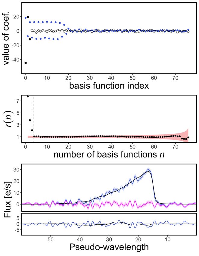
A&A 652, A86 (2021)

                                                                      second one will observe it afterwards (the following FoV). The
                                                                      light from these two different telescopes is projected onto a com-
                                                                      mon focal plane with charge-coupled device (CCD) detectors.
                                                                      For the case of the Gaia spectrophotometers, after being dis-
                                                                      persed by two different slitless prisms, the light is collected by
                                                                      one set of CCDs for each spectrophotometer (with seven CCD
                                                                      rows2 across the focal plane, see Fig. 2). The spectral range cov-
                                                                      ered by the two spectrophotometers is different. The blue pho-
                                                                      tometer (BP) covers the short wavelengths in the 330–680 nm
                                                                      range, while the red photometer (RP) covers longer wavelengths,
                                                                      in the 640–1050 nm range.
                                                                           In order to reduce the telemetry of the satellite, only a small
                                                                      window around the detected position of the source is downloaded.
                                                                      The size of the window (60 pixels × 12 pixels = 3.5 arcsec ×
                                                                      2.1 arcsec) around the spectra was selected to be wide enough to
                                                                      include most of the flux from the source once dispersed by the
Fig. 1. Scheme used to calibrate Gaia spectrophotometry. This paper   spectrophotometric prisms and also contain a range of pixels for
only deals with the internal calibration piece (dashed square).       background flux determination. The longer size of the BP and
                                                                      RP windows (60 pixels, equivalent to 3.5 arcsec) in comparison
                                                                      with the window scheme used for the astrometric field observa-
absolute fluxes and wavelengths. This paper describes the con-
                                                                      tions (only 12 or 18 pixels wide, equivalent to 0.7 and 1.1 arcsec,
cepts of the internal calibration of Gaia spectrophotometric data,
                                                                      respectively) implies a higher chance of overlapping windows
but this is not linked to the particular details used in any of the
                                                                      (triggering truncation) and blends (where more than one source
Gaia data releases. Different papers will be published, together
                                                                      is captured in the same window).
with Gaia DR3 and future releases, with the particular details
                                                                           As previously mentioned, Gaia is spinning on itself in order
of the actual model used to produce that particular dataset (i.e.,
                                                                      to scan all of the sky. This spinning process causes the images of
giving the actual used basis functions for the source represen-
                                                                      the sources in the sky to transit the focal plane during the obser-
tation, the set of calibrators, the instrument model parameters,
                                                                      vation. We refer to the transit direction as ‘along scan’ (AL). The
etc.). Pre-processing and external calibration procedures also fall
                                                                      perpendicular direction to AL is called ‘across scan’ (AC). Each
outside the scope of this paper.
                                                                      CCD is operated in time delay integration (TDI) mode to com-
    The internal calibration (Sect. 3) models the instrument with-
                                                                      pensate for this spinning effect. TDI mode consists of reading the
out the use of external information, working entirely in the
                                                                      image not at the end of a predefined time exposure, but continu-
instrument system. The way to proceed without external infor-
                                                                      ously at a given rate. The charges are clocked through the CCD
mation is to study how a set of (assumed constant) calibration
                                                                      in the AL direction at a constant rate, and the satellite rotation is
sources (Sect. 6) produce different observations when obtained
                                                                      constantly adjusted to make the images move at the same rate as
with different instrumental conditions: how they change with
                                                                      the reading takes place. With this procedure, the light from every
time, the focal plane position, detector used, field of view (FoV),
                                                                      source is integrated during the transit over every CCD.
and so on. Section 2 explains these instrumental effects and
                                                                           The result for Gaia is that the observed source transits each
how the key point when performing the internal calibration is
                                                                      CCD in about 4.4 s (this being the maximum exposure time of
to model the relative differences among observations (in terms
                                                                      each observation). The use of ‘gates’ limits the region of the
of dispersion, line spread function, sensitivity, etc.), not their
                                                                      CCD to be read, effectively limiting the exposure time in case the
absolute values. As neither the instrument nor the sources are
                                                                      source is too bright. Each of the CCDs has 4500 pixels in the AL
known in advance, this process needs to determine both iter-
                                                                      direction and 1966 pixels in the AC direction. The recording pro-
atively (Sect. 4). Sections 3 and 5, respectively, describe the
                                                                      cess of the BP and RP spectrophotometry with the CCD devices
models representing the instrument and the sources, defining
                                                                      produces a pixelisation of the spectra that is highly dependent
some parameters to be determined during the calibration pro-
                                                                      on the geometry of the CCD and its pixels, the allocation of the
cess. Section 7 shows preliminary results of the internal calibra-
                                                                      reading window around the observation, and so on.
tion model explained here. Finally, Sect. 8 includes a summary
                                                                           The 2D image of the spectra in BP and RP is collapsed
and conclusions of this work.
                                                                      into 1D spectra, binning the pixels in the AC direction while
                                                                      being read for observations fainter than G = 11.5 mag. This
                                                                      introduces the concept of a ‘sample’, corresponding to a group
2. The Gaia spectrophotometers                                        of 12 pixels in the AC direction once combined to constitute
In this section, we briefly review the Gaia spectrophotome-           the 1D spectra. In this way, these 1D spectra are composed of
ters and the instrumental effects affecting the observations          60 different samples. Nevertheless, the outermost ten samples
to be calibrated, and we refer the reader to several previ-           (approximately) on either side of the window correspond to a
ous papers where more detailed descriptions of these effects          negligible instrumental response, and the signal there is domi-
can be found (Gaia Collaboration 2016, 2018a; Riello et al.           nated by background flux and the smearing effects of the line
2021; Hambly et al. 2018; Crowley et al. 2016; Fabricius et al.       spread function (LSF).
2016 and Carrasco et al. 2016). Here, we are only interested in            The calibration of the spectrophotometric observations is
describing the concepts needed in our modelling (see Sect. 4).        complicated due to intrinsic variations of the instrumental con-
    The Gaia satellite collects the light from two different tele-    ditions for different observations. The Gaia focal plane is very
scopes (FoVs). As Gaia is spinning while observing the sky,
in one of these revolutions one of these telescopes (the leading      2
                                                                         We use CCDs 1 to 7 to refer to the different CCD rows in the spec-
FoV) is always first to observe a region in the sky, while the        trophotometric instrument.

A86, page 2 of 20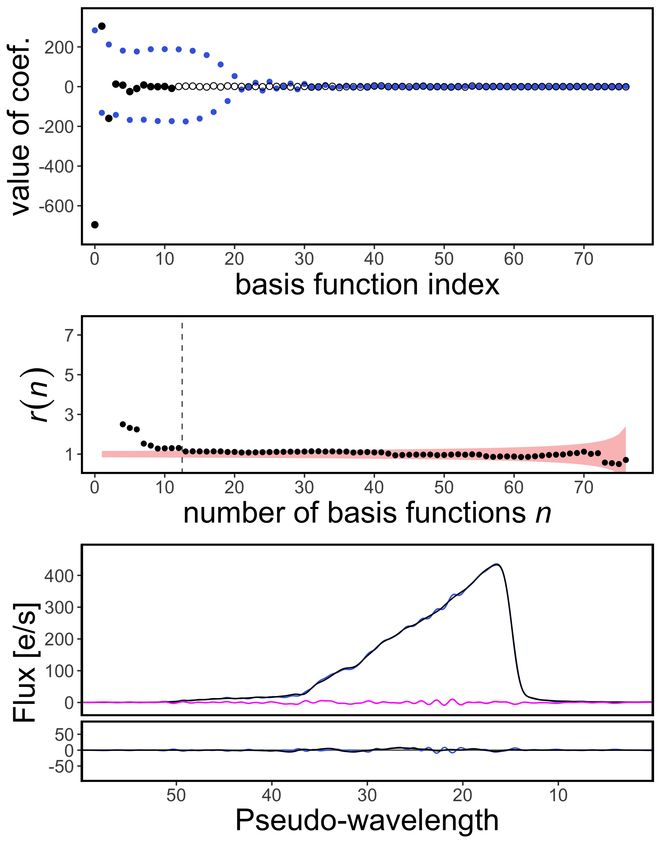
J. M. Carrasco et al.: Internal calibration of Gaia BP/RP low-resolution spectra
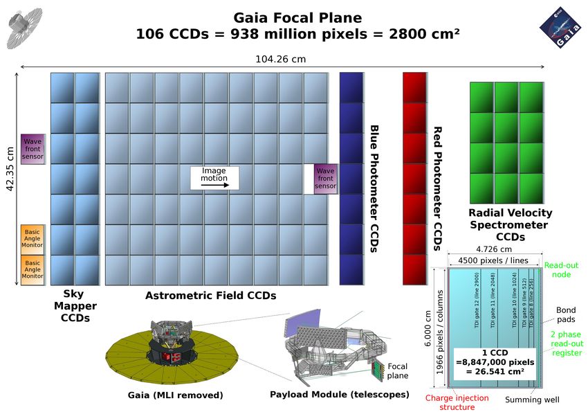
Fig. 2. Gaia focal plane. For the photometric calibration explained here, only CCDs in the blue and red photometers are relevant (picture courtesy
of ESA – A. Short).
large3 , with a large number of CCDs4 , two overlapping FoVs of these two instruments is lower than 100 and depends on the
(with their different optical paths), the occurrence of gates and wavelength range and the position in the focal plane (see Fig. 3,
window strategies, and the instrumental behaviour changing top). Although similar, the dispersion law for the two different
with time. The main instrumental ingredients to be considered FoVs is also different. The variation of the dispersion law with
for the calibration of the Gaia spectrophotometry are geometry, the position in the focal plane also causes the length of the spec-
dispersion, LSF, sensitivity and flux loss. We explain them in tra to be different on different CCDs (see Fig. 3, bottom).
detail in the following paragraphs. The resolution of the instrument was chosen to be able to
The geometric calibration deals with the fact that different reproduce the passbands described in Jordi et al. (2006). In spite
spectra obtained at different positions of the focal plane are not of this low resolution, the amount of science potentially avail-
perfectly aligned. We need to know the differences in the actual able for so many sources in all the sky with homogeneous spec-
projection of the spectra on the detectors. The dispersion direc- trophotometric observations is very promising. This is noted, for
tion may also not be perfectly aligned with the transit direction, example, in Sect. 7, where some calibrated spectra for sources
and thus some tilt could be present. This will produce a discrep- with different colours are shown, making it possible to distin-
ancy between the expected position in the CCD of a given wave- guish their different spectral energy distributions. The astrophys-
length and the actual one. The instrumental model explained in ical parameters derived from the calibrated spectrophotometry
this work can cope with small spectral misalignments in the AL will also be published with the next Gaia DR3 catalogue.
direction (limited by the maximum number of neighbours con- Besides the variation of the dispersion properties at different
sidered in the model, see Sect. 3), but larger misalignments need positions across the focal plane, the wavelength range at differ-
to be corrected by pre-processing before our model is applied. ent positions can be slightly different because of the passband
The spectral dispersion could also be different for different differences, providing different widths for the spectra. Table 1
observations. As the initial purpose of the two spectrophotome- shows the cut-on and cut-off wavelengths (λcuton and λcutoff
ters is mainly to provide the chromatic centroid correction in respectively), which translates to different total bandwidths in
astrometry (Lindegren et al. 2018, 2021) as a function of the wavelengths (∆ = λcutoff − λcuton ). Due to these effects, the corre-
spectral energy distribution of the source, the spectral resolution spondence between samples and wavelengths will vary for dif-
ferent observations of a given source. Furthermore, the spectral
3
The full Gaia focal plane is 104 cm × 42 cm. BP and RP CCDs also
dispersion is also expected to change with time. All these disper-
cover a length of 42 cm, but they are limited to the size of one single sion variations (summed to the more important effect of the AL
CCD strip (of about 4.5 cm wide). centring of the windows previously explained) prevent us from
4
The full Gaia focal plane comprises 106 different CCDs. Among naively summing the different epoch spectra to obtain a mean
them, each BP and RP instrument uses seven different CCDs. spectrum.
A86, page 3 of 20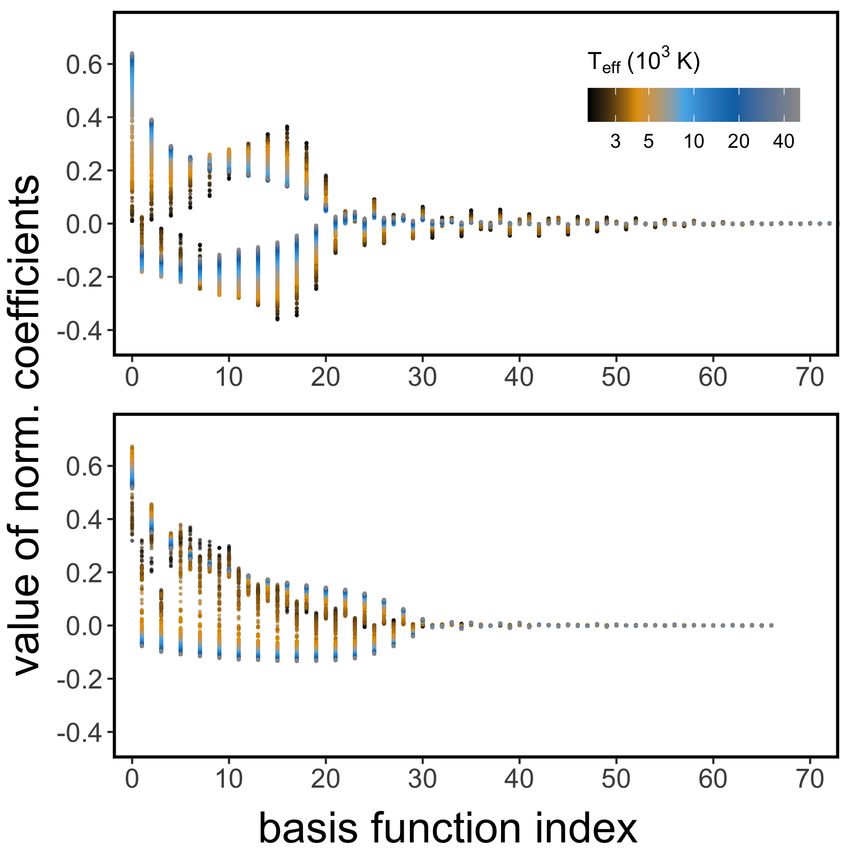
A&A 652, A86 (2021)

                                                                           Fig. 4. Correspondence between the absolute wavelength and pseudo-
                                                                           wavelength scale for simulations in BP (black) and RP (orange) used in
                                                                           this paper for CCD7. These are only intended to be used as indicative
                                                                           values for the reader.

Fig. 3. Top: nominal spectral resolution relationship (https://www.
cosmos.esa.int/web/gaia/resolution) with wavelength (λ). ∆λ
is the width of a spectrophotometric sample for BP (shorter wave-
lengths) and RP (longer wavelengths) spectrophotometers for the pre-
ceding telescope. The colour scale indicates how this resolution changes
with the AC position in the focal plane. Bottom: length of the BP (black
lines) and RP (orange lines) spectra for different CCDs and FoVs com-
pared with the length in CCD1.

Table 1. Bandwidth variations in different Gaia CCDs.

                                   BP           RP                         Fig. 5. LSF at three different wavelengths (525 nm at MgH band in the
                                                                           bottom panel, 750 nm at pseudo-continuum region in the central panel,
                λcuton [nm]     397–399      629–631                       and 775 nm at TiO band in the top panel). In each panel, three different
                λcutoff [nm]    665–668      918–919                       CCDs are plotted, corresponding to the bottom (CCD1 in black), middle
                  ∆ [nm]        266–270      287–290                       (CCD4 in blue), and upper (CCD7 in orange) positions of the focal
                                                                           plane, respectively.

    Once the geometric calibration and a rough dispersion law              image of a point-like source obtained with a telescope is not a
is known, we can define an internal reference scale, referred to           point, but it has some spread on the focal plane. The final image
as ‘pseudo-wavelength’. We call it pseudo-wavelength because               of this point obtained by the detector is known as PSF. The LSF
it does not yet have the usual physical units for wavelengths              can be understood as analogous to the PSF when collapsed into
(nanometres, for instance), but it is measured in units of sample          1D. When this concept is applied to spectroscopic images, the
in an arbitrarily chosen reference location in the focal plane (AL         result is that the light with a given wavelength is not registered
positions in the 1D window for a given CCD and AC coordinate).             only in a single pixel, as desired, but in several, depending on
The external calibration will produce the transformation to the            the width of the LSF (1–2 pixels wide, see Fig. 5). This pro-
physical units. As a reference, pseudo-wavelength values 10 and            duces some contamination of the adjacent pixels by light with
50 approximately correspond to wavelengths 860 and 330 nm in               wavelengths nominally corresponding to the neighbouring pixels
BP and 630 and 1090 nm in RP (see Fig. 4). In the internal cal-            according to the dispersion law. This effect (sometimes referred
ibration process explained in this work, this pseudo-wavelength            to as the alien photon problem) changes with wavelength, the
scale is sufficient in order to align the observed spectra and form        position in the focal plane (see Fig. 5), the FoV, and time.
the mean spectra from various observations of a given source                   Therefore, the smearing of the spectrum will be different
obtained at different locations of the focal plane, FoV and time.          for each observation. Figure 6 illustrates this, showing first the
The external calibration step (see Fig. 1) provides the relation           dispersion and LSF effect alone (left and central panels) and
between pseudo-wavelengths and true wavelengths.                           then combining them in the right panel. The simulations in
    Due to diffraction, aberrations, and further non-optical               Fig. 6 were produced using the Gaia Object Generator (GOG,
effects, such as the CCD pixelisation or spacecraft motion, the            Luri et al. 2014). The evolution of the contamination of the
A86, page 4 of 20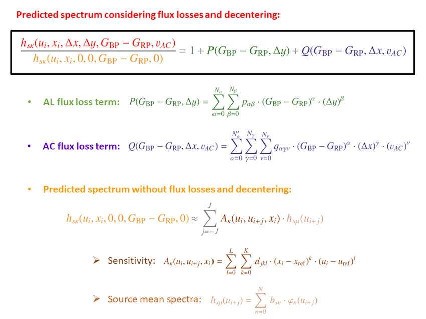
J. M. Carrasco et al.: Internal calibration of Gaia BP/RP low-resolution spectra

Fig. 6. RP simulations, using the synthetic spectral energy distribution library of Lejeune et al. (1997), of the effect of ±10% dispersion variation
(left), LSF conditions in the seven CCDs (centre), and both effects together as expected in each CCD (right), for a star with an effective temper-
ature of T eff = 3350 K. The ±10% dispersion variation considered in the left plot represents the maximum variation expected for the different
observations. The dispersion at a given time of the mission changes across the focal plane with the CCD. The latter effect is included in the plot at
the right.

mirrors, refocussing events and changes due to environmental                change by about 0.8%–1.4% when shifting the window ±2 pix-
conditions (such as the effects of the decontamination events)              els in the AC direction and considering different AC motion due
affect the LSF (see Riello et al. 2021; Rowell et al. 2021 and              to the intrinsic motion of the astrophysical source and the satel-
Mora et al. 2014).                                                          lite attitude. The effect of the AC shift does not depend much
     Flat field images cannot be obtained during the Gaia mis-              on the colour of the source and the variations are smaller than
sion to measure sensitivity variations, as is commonly done with            0.05%, meaning that the variation is almost grey.
on-ground instruments. The only flat field information available                 In the case of the AL flux loss, the variation in flux is limited
was obtained before launch for the sole purpose of obtaining                to 0.5% when a ±3 pixel shift in the AL direction is considered.
an estimation of the instrument’s behaviour. It is not suitable to          This AL flux loss can change with colour (0.2%–0.6% in BP
describe the sensitivity variations during the mission. The dif-            and 0.2% in RP). The maximum variation between CCDs of the
ferent episodes of contamination on the mirrors and the detec-              flux inside the window is about ±0.02–0.03% in the case of an
tors, the decontamination events, and the expected ageing of the            AL shift= +1 (i.e., very little compared with changes due to AC
optics and CCDs (see Riello et al. 2021) make these pre-launch              shifts). These estimations do not account for the extra losses due
estimations insufficient for covering the mission. The response             to bad focus periods during operations.
of the instrument to a given wavelength will be different for dif-               Observations in different FoVs meet partially separate opti-
ferent FoVs, CCDs, gates, and positions on the CCD. As the                  cal surfaces and have different optical paths, which may result
observation is integrated in the AL direction, only the AC posi-            in different dispersed LSFs and response functions. Gated inte-
tion (column) in the CCD is relevant here for the sensitivity               gration over a different section of the CCD for bright sources
analysis. Within each CCD, a column response non-uniformity                 implies different dispersed LSF and response conditions. To take
(CRNU) of a few per cent is present (Crowley et al. 2016).                  this complexity in the Gaia spectrophotometers into account,
     Figure 7 shows some examples of these CRNU images                      we propose the calibration model explained in the following
obtained before launch. The lower pixel responses are found                 sections.
at the corners of the CCD. The sensitivity variation is mostly                   The presence of blended observations, non-perfect bias
smooth with the column, except at the stitch boundaries inside              and background subtraction, charge injection events, dead
the CCD. The stitch boundaries are the result of the fact that a            pixels, and other non-linear effects such as saturation and
given CCD is produced in several photo-lithographic units. The              charge distortion complicates the calibration process even more
separation between these parts produces small jumps in the sen-             (see Riello et al. 2021; Evans et al. 2018; Hambly et al. 2018;
sitivity of the device in neighbouring columns. Moreover, dead              Crowley et al. 2016 and Fabricius et al. 2016 for more details).
pixels or hot ones can also produce variations in the flux obtained         The calibration pipeline must account for as many of these
at discrete positions. A degradation of the sensitivity with time           effects as possible, or at least try to evaluate the extra uncer-
is also to be expected.                                                     tainty in the final result if they are not considered. Another (or
     The flux loss is the combination of the LSF effect with the            complementary) approach is to simply reject some of the obser-
limited extension of the window around the source being trans-              vations affected by these unaccounted effects as outliers, if they
ferred to ground. It results in part of the light of the spectra being      represent a small part of the observations for that source. The
lost in our measurements. The imperfect centring of the window              remaining observations of a given source can be used to build
around the source also increases the amount of flux loss.                   a mean spectrum, which will reduce the uncertainty in principle
     By simulating observations with nominal LSFs we can esti-              by a factor equal to the square root of the number of observations
mate the influence of the flux loss in Gaia spectrophotometry.              considered.
The total amount of flux lost outside the window is about 4–5%                   The number of observations for a given source depends
in the case of BP and 4.5–5.5% in the case of RP. The reason for            on the satellite scanning law, and the probability of detecting
having more flux outside RP windows is that the LSF is wider                a source depends on its magnitude and the crowding in the
for larger wavelengths. Added to this, the centring error in the            observed region of the sky (also considering the second FoV,
RP observations is slightly larger due to the RP zooming effect             which overlaps in the same focal plane). On average, a source in
(see Riello et al. 2021), producing a larger flux loss than in BP.          the Gaia catalogue will have about one hundred observations
     The relevant parameter for the internal calibration is the vari-       in five years. The very large volume of data to be processed
ation of the flux loss in different observations. The flux loss can         adds to the challenge. For reference, by the time of Gaia EDR3

                                                                                                                                  A86, page 5 of 20
A&A 652, A86 (2021)
Fig. 7. Column response non-uniformity (CRNU; Kohley et al. 2009). Dependence of the response of the CCD detector as a function of the AC
position (column) and CCD for BP (left) and RP (right) for three different wavelengths (in different colours). Some abrupt changes in neighbouring
AC positions can be observed in the different CCDs due to stitch block discontinuities.
(December 2020), more than 300 billion spectrophotometric I(u, λ, ω1 , . . . , ωΩ ) = Λ (u(λ, ω1 , . . . , ωΩ ), λ) R(λ, ω1 , . . . , ωΩ ).
observations had been obtained5 , all of them under different (2)
instrumental conditions. Given the size and complexity of the
task, a priority requirement is to keep the load on the computer The goal of the internal calibration is to characterise the dif-
systems at a feasible level using a robust pipeline. ferences among all the observations, removing the dependence
on the Ω parameters ω1 , . . . , ωΩ , such that all epoch spectra are
described by an integral transformation with a kernel Iµ (u, λ),
3. Basic formulations not depending on the parameters ω1 , . . . , ωΩ and identical for all
In this section and the following one we establish the main equa- observations. If this is achieved, we considered all observations
tions of the model, which are summarised in Fig. 8. BP and to be reduced to a common instrument (µ), which we refer to as
RP spectra of the Gaia mission are internally calibrated inde- the mean instrument. This term does not however imply a mean
pendently of each other. The calibration approach is exactly the in any mathematical sense, and it is not uniquely defined. Any
same, however. In order to be concise, we do not refer to BP and kernel independent of the instrumental parameters ω1 , . . . , ωΩ
RP spectra or BP- and RP-specific indices. Instead, we simply can in principle serve as a mean instrument.
speak of ‘spectra’, which can mean either the BP spectra or RP To remove the dependence on the ω1 , . . . , ωΩ , we may first
spectra. separate the continuous parameters into intervals with similar
The different instrumental properties (Sect. 2) drive the conditions. The boundaries of the intervals can be chosen at (or
obtained epoch spectrum of a given source. We define close to) discontinuities. For the time parameter, such bound-
ω1 , . . . , ωΩ as the set of Ω parameters needed to describe the aries may be the times of decontamination or re-focussing of the
instrument influence on the epoch observation. The parameters telescopes (see Fig. 5 in Riello et al. 2021). For the AC posi-
ω1 , . . . , ωΩ required to describe the differences among instru- tion parameter, it may be the boundaries between CCDs or stitch
ments and, consequently, the epoch spectra, can either be contin- blocks of a CCD. Each combination of a particular interval of the
uous (for example, time variations and AC position variations) or continuous parameters and the discrete parameters we refer to as
discontinuous or discrete (FoV, gates, window class, decontami- a calibration unit. Within each calibration unit, the instrument
nation and refocusing events, CCD stitch blocks, etc.). only shows, by construction, a smooth variation.
We may write the epoch spectrum for a source, s, in a For the moment, we assume that the smooth variations inside
given pseudo-wavelength, u, as hs (u, ω1 , . . . , ωΩ ). We further- a given calibration unit are negligible, and we come back to them
more assume that each epoch spectrum is linked to the spectral later. We may index the calibration units with an index κ, with
photon distribution (SPD, S (λ)) as a function of the wavelength, some arbitrary but fixed ordering. To any index κ, there are inter-
λ, of the source via an integral transformation of the form vals in the continuous parameters and particular values of the
discrete parameters assigned to it. Then, we may link any epoch
Z∞ spectrum in κth calibration unit with the SPD via
hs (u, ω1 , . . . , ωΩ ) = I(u, λ, ω1 , . . . , ωΩ ) · S (λ) dλ . (1) Z∞
0 hsκ (u) = Iκ (u, λ) · S (λ) dλ, (3)
The integral kernel I(u, λ, ω1 , . . . , ωΩ ) describes the instru- 0
ment and contains the influence of the Ω instrumental parame-
ters mentioned above. I(u, λ, ω1 , . . . , ωΩ ) may be separated into with Iκ (u, λ) being the instrument kernel for the κth calibra-
the contributions from the response function, R, and the LSF , Λ, tion unit, where, as previously stated, we neglected the inter-
which also includes the dispersion relation (linking u and λ), as calibration unit variations for the time being and did not consider
dependency of the Iκ (u, λ) on the ω1 , . . . , ωΩ parameters.
5
We refer the reader to an updated estimation for the number To be able to internally calibrate the instrument at all, we
of observations in each Gaia instrument at https://www.cosmos. have to assume that for each calibration unit, a linear transfor-
esa.int/web/gaia/mission-numbers. mation exists between the epoch spectra in the κth calibration
A86, page 6 of 20J. M. Carrasco et al.: Internal calibration of Gaia BP/RP low-resolution spectra
Fig. 8. Summary of the equations explained in Sects. 3 and 4. The meaning of the variables is detailed in the text and in Table A.2.
unit, and the mean internal instrument, µ, which can, but does We can thus express the epoch spectrum in κth calibration unit as
not necessarily have to be, one of the calibration units. a linear combination of basis functions with the same coefficients
Since all linear transformations between well-behaved math- used for the mean spectrum, and with the basis functions in κth
ematical functions can be uniquely expressed by an integral calibration unit being the basis functions chosen for the mean
transform, we may choose to express the transformation between instrument transformed by the application of Aκ .
the mean instrument µ and the κth calibration unit as an integral For practical computations, we can approximate the integral
transform, using a transformation kernel Aκ , which thus has the in the equation above using Riemann sums, meaning we use the
following form: following approximation:
N ∞
Z∞ X X
hsκ (ui ) ≈ bsn Aκ (ui , u j ) · ϕn (u j ). (8)
hsκ (u) = Aκ (u, u ) · hsµ (u ) du .
0 0 0
(4) n=0 j=−∞
−∞
We may introduce a second approximation, namely that the ker-
For the mean spectrum hsµ (u), we chose a continuous repre- nel Aκ describing the transformation between the mean instru-
sentation by a linear combination of basis functions, ϕn (u) (see ment and the κth calibration unit is localised. The scale over
Sect. 5). Thus, for a particular source, we assumed which variations in a spectrum are correlated at different u is
determined by the width of the LSF, and the LSF itself is a
N
X localised function. We may therefore achieve a good approxi-
hsµ (u) = bsn · ϕn (u), (5) mation to truncate the infinite summation to finite limits around
n=0 each discrete point i. We obtain
with bsn the coefficients of the spectrum of a source s in the finite N
X J
X
development with N + 1 basis functions. We highlight that there hsκ (ui ) ≈ bsn Aκ (ui , ui+ j ) · ϕn (ui+ j ). (9)
is a single set of bsn coefficients for a given source, independently n=0 j=−J
of the epoch and calibration unit of their observations. Inserting
Eq. (5) into Eq. (4) gives This expression is essentially a discrete convolution of the mean
spectrum to obtain the different epoch spectra (which correspond
Z∞ N to different κth calibration units), with the generalisation that the
discrete convolution kernel Aκ (ui , ui+ j ) is not only a function of
X
hsκ (u) = Aκ (u, u0 ) bsn · ϕn (u0 ) du0 (6)
n=0
ui − ui+ j , but of both ui and ui+ j individually. Aκ (ui , ui+ j ) may
−∞
therefore vary with u during the discrete convolution process.
N
X Z∞ We chose Eq. (9) as the basic formulation of the internal instru-
= bsn Aκ (u, u0 ) · ϕn (u0 ) du0 . (7) mental calibration model for Gaia’s spectra, which consists of
n=0 −∞ determining Aκ once the set of source basis functions is fixed.
A86, page 7 of 20A&A 652, A86 (2021)
Fig. 9. Graphics showing contribution from neighbouring pixels for
J = 2 case in Eq. (9). This influence from neighbouring pixels needs
to be taken into account when predicting the observation hsκ in the κth
calibration unit starting from the reference mean spectrum hsµ . Fig. 10. Change in the value of the coefficients when different AL shifts
(from −3 to +3) are considered for the observations with respect to the
mean spectra. No dispersion and LSF effect variations are considered
The nature of the discrete convolution with a variable ker- between the mean spectra and the observation.
nel is illustrated in Fig. 9. For any given sample ui of the spec-
trum, the calibrated spectrum results from an exchange of flux
between neighbouring samples ui+ j , where the index j runs over
the finite range −J to J. The discrete kernel Aκ (ui , ui+ j ) describes
the amount of exchange of flux between the samples ui and ui+ j
when transforming the mean spectra into the epoch spectra.
Due to the limitation imposed on the jth interval, the maxi-
mum flux influence of the neighbours is limited to ±J. The cho-
sen value for J should be selected based on the expected influ-
ence of the neighbouring fluxes. As we see in Sect. 2, the width
of the LSF and dispersion difference between calibration units
recommend the choice of J to be at least two neighbours or more
(J ≥ 2).
The choice of J will also limit the maximum AL shift allowed
to compare different observations. If some shift is present, the
derived Aκ values will incorporate this effect to account for this
shift. For instance, Fig. 10 shows how the derived values of these
coefficients change when the only difference between the mean
spectra and the observations are due to AL shifts (no dispersion Fig. 11. Change in the value of the coefficients when different Gaia BP
and LSF changes are introduced in this test and thus only j = 0 CCDs (with different dispersion and LSF conditions) are considered
contribute here, Aκ = 1, and the rest of neighbours are zero). for the observations with respect to the mean spectra. The cases of the
mean spectra in the CCD1 reference system and observations in CCDs
Although keeping the shape of the Aκ values was not imposed, the
1 (black), 4 (orange), and 7 (blue) are plotted here.
algorithm detects that only a shift of the values is needed to repro-
duce the shift introduced to the spectra in the AL direction. The
range of AL shifts that the model is able to cope with are limited Since we do not expect abrupt changes of the kernel with ui ,
to the J value (the maximum number of neighbours, J = 3 in this a low-order polynomial may be a suitable choice as a basis. In
case in Fig. 10). As one of the previous steps in the pre-processing this case, we obtain a parametrisation:
is the calibration of the CCD geometry (see Fig. 1), we do not
L
expect to see significant shifts in the internal calibration. This geo- X
metric calibration of the spectra was already done in previous data Aκ (ui , ui+ j ) = c jl · (ui − uref )l . (11)
releases when using the spectrophotometric data to derive the pho- l=0
tometric calibration (Carrasco et al. 2016). If instead of producing The value of uref is a reference pseudo-wavelength that may
a shift we perform the prediction of an observation in a different be chosen in any convenient way (for example, the centre of
calibration unit in Gaia with different dispersion and LSF condi- the window or one of the extremes, once the different spectra
tions among the mean spectra and the observation, this produces have been aligned with the previous geometric calibration pro-
a deformation of the Aκ coefficients (see Fig. 11) with respect to cedure). This approach reduces the number of coefficients to be
the simple shape seen in Fig. 10. fitted and improves the physical interpretation of Aκ , reducing
Aκ (ui , ui+ j ) is assumed to be a smooth function of ui . For a degeneracies.
compact representation of the kernel Aκ (ui , ui+ j ), we may choose Until this point, we neglected the possible smooth variation
to represent its dependence on ui as a linear combination of basis of the instrument in time and AC position within a particular
functions (E). We thus use a development of the following form: kth calibration unit. At this point, we are able to take such vari-
L
X ations into account. This we do by introducing a polynomial
Aκ (ui , ui+ j ) = c jl · El (ui ). (10) dependence of the c jl coefficients on the AC position, xi , for the
l=0
pseudo-wavelength ui with respect to a reference AC position,
A86, page 8 of 20J. M. Carrasco et al.: Internal calibration of Gaia BP/RP low-resolution spectra
xref , as follows: mean spectra of the internal calibrators. The simplest approach is
to assume no differences between the different calibration units,
K
X hence using the identity transform between the mean instrument
c jl = d jkl · (xi − xref )k . (12) and all calibration units:
k=0
d jkl = δ j0 δk0 δl0 (15)
This results in the expression
L X
K
with δαβ being the Kronecker delta. This is the behaviour shown
X in Fig. 10 when no change (in shift, dispersion, LSF, etc.) is con-
Aκ (ui , ui+ j , xi ) = d jkl · (xi − xref ) · (ui − uref ) .
k l
(13)
sidered between the mean spectra and the observation scales.
l=0 k=0
With this initial guess for the instrument parameters, Eq. (14)
Combining this equation with Eq. (9), we obtain the follow- can be solved for the coefficients bsn for all internal calibrators.
ing expression to derive the prediction of the epoch spectra hsκ In a following step, the bsn can be kept fixed, and Eq. (14) can
for κth calibration unit in a pseudo-wavelength ui and located at be solved to obtain the instrumental parameters d jkl . The itera-
the AC position xi , tive process of source update and instrument update can continue
until convergence is reached.
X J X
N X K X
L To ensure convergence, two additional considerations can
hsκ (ui , xi ) ≈ bsn · d jkl · (xi − xref )k · (14) be introduced. First, the epoch spectra predicted by the model
n=0 j=−J k=0 l=0 remain the same if the source coefficients, bsn , are multiplied
× (ui − uref )l · ϕn (ui+ j ). by an arbitrary scaling factor, and the instrumental coefficients,
d jkl , are divided by the same scaling factor. This effect corre-
Time variations of the instrument are dealt with by solving sponds to a degeneracy between the instrumental response and
the instrument model in specific time intervals, meaning we used the flux scale of the mean spectra. If this effect is producing a
observations taken within a given time range. These time ranges divergence of the solution, this can be mitigated through a re-
are treated as another calibration unit with different instrumental normalisation of the instrumental parameters after every instru-
conditions. The lengths of these intervals need to be longer when ment update. This can be introduced by dividing the instrumental
calibrating gated and 2D observations due to the limited number kernel by their sum over all neighbours, AC positions, and cali-
of observations obtained in these configurations. bration units.
We refer to the process of determining the instrumental coef- Secondly, all κ calibration units are required to converge
ficients, d jkl , as an ‘instrument update’, keeping the coefficients to the same mean instrument; that is, systematic differences
of the calibration sources in the representation of the mean spec- between the mean spectra of two sources with identical SPDs
tra, bsn , fixed. On the other side, the mean spectra of the source but a different distribution of their observations in calibration
are known when bsn coefficients are determined. We refer to the units need to be avoided. This can be achieved by employing
derivation of these bsn coefficients for all calibration sources as sources with observations in several different calibration units.
‘source updates’, keeping the instrumental parameters, d jkl , fixed One example of this is the use of sources observed with differ-
(see Fig. 1). Once the instrumental coefficients are known with ent gating conditions. This kind of source will ensure the con-
the calibration sources, the same d jkl values can be applied to the vergence of the solution for the different gates to a common
rest of sources (non-calibrators). reference system without sudden jumps in the behaviour of the
calibrated instrument with magnitude. Further considerations on
the selection of the internal calibrators are included in Sect. 6.
4. Instrument calibration An additional complication of the internal calibration pro-
cess results from the observation of a window of finite size
The determination of the instrument coefficients, d jkl in Eq. (14), around the expected position of a source on the CCD. This
requires the knowledge of the bsn coefficients representing the limited size of the window added to the inaccurate centring of
sources as in the mean instrument. Ideally, these coefficients the source within the window and AC motion (as discussed in
are known for M calibration sources, with M being sufficiently Sect. 2), means that the observed spectrum only includes a frac-
large (of the order of millions for the Gaia case). We refer tion of the flux of a particular source. A correction for the flux
to these sources as the ‘internal calibrators’. However, before loss is included within the internal calibration procedure.
the instrument calibration is performed, the representation of The source can be de-centred within the window by a certain
sources in the mean instrument is unknown. To overcome this amount in AL and AC directions (∆y and ∆x, respectively). We
deadlock, an iterative approach was adopted. We may assume evaluated, using pre-flight simulations, the expected contribution
either the coefficients of the internal calibrators in the mean of the flux loss due to AL and AC shifts, the colour of the source
instrument (bsn ) to be known and derive the parameters describ- (GBP −GRP ), and AC motion (vAC ). Based on these results, we
ing the transformations to the different calibration units (d jkl ), or can apply a model splitting the contributions to the flux loss into
we may assume the opposite scenario, in which the instrumen- different components:
tal kernel to transform between the different calibration units is
known, and derive the source coefficients of the internal cali- hsκ (ui , xi , ∆x, ∆y, GBP − GRP , vAC )
brators in the mean instrument. These steps can be applied iter- = 1 + P + Q, (16)
hsκ (ui , xi , 0, 0, GBP − GRP , 0)
atively, and the convergence can be monitored from the agree-
ment between the epoch spectra of the internal calibrators and with hsκ (ui , xi , ∆x, ∆y, GBP − GRP , vAC ) being the flux once the
their predictions, derived from the mean spectra and using the losses have been accounted for and P and Q the AL and AC flux
transformation obtained between the mean instrument and the loss contribution, respectively: both of them defined as negative
epoch spectra. and represented here by two polynomial functions (Eqs. (17)
Starting this iterative process requires some initial values, and (18)). hsκ (ui , xi , 0, 0, GBP − GRP , 0) is the calibrated flux
either for the parameters describing the transformations, or the obtained from Eq. (14) without considering flux loss.
A86, page 9 of 20A&A 652, A86 (2021)
We used a polynomial representation for both P and Q func- allowing us to compute any higher order Hermite function. Basi-
tions on their dependences. The AL flux loss, P term in Eq. (16), cally, the Hermite functions arise from Hermite polynomials by
does not depend on the AC motion (vAC ): multiplication with a Gaussian function. As a result, they are
Nβ
Nα X
centred at θ = 0, and for sufficiently high θ absolute value,
all Hermite functions are converging to zero. This resembles
X
P(GBP − GRP , ∆y) = pαβ · (GBP − GRP )α · (∆y)β , (17)
the global behaviour of Gaia’s spectrophotometry, which is also
α=0 β=0
converging to zero for focal plane positions sufficiently far from
but the AC flux loss does: the location of the source.
0 Nγ X
Nα X Nν Hermite functions are furthermore orthonormal with respect
to each other, meaning they satisfy the following orthonormality
X
Q(GBP − GRP , ∆x, vAC ) = qαγν (GBP − GRP )α (∆x)γ (vAC )ν .
α=0 γ=0 ν=0
condition:
(18) Z∞
Nβ , Nγ and Nν are, respectively, the degree chosen for the ϕn (θ) · ϕm (θ) dθ = δnm . (22)
dependence on AL and AC centring error and AC motion. Nα −∞
and Nα0 represent the degree for the polynomial dependence on
the colour for the AL and AC flux loss terms, respectively. The As the Hermite functions are centred on θ = 0, the origin of
typical values for the maximum degree of dependence with all the pseudo-wavelength axis, u, should be shifted such that the
these parameters are not expected to be larger than first or second origin becomes close to the centre of the spectra. Furthermore,
order polynomials, according to the evaluations of these effects the pseudo-wavelength axis needs to be re-scaled such that the
explained in Sect. 2. Although we mention in Sect. 2 that the width of the spectra is met to the width of Hermite functions. We
AC flux loss dependence with colour is not very critical (almost therefore consider a linear transformation between the pseudo-
grey compared with the dependence on the AL flux loss) and wavelength axis u and the argument of the Hermite functions θ
that most of the colour dependence is accounted for in the AL of the form
flux loss equation, Eq. (17), we prefer to keep the colour depen-
dence in the AC flux loss model, Eq. (18), to account for its small θ = Θ · u + ∆θ . (23)
dependence if needed, but it could be neglected (setting Nα0 = 0) The scaling parameter Θ, the shift ∆θ, and the number of basis
if this dependence is found to not be important. functions N need to be determined based on actual spectra. The
three parameters may, however, not be chosen independently of
5. Representation of the mean spectra each other. If a spectrum has to be represented over a certain
range of pseudo-wavelengths, then choosing a smaller scaling
To choose the basis functions ϕn (u), n = 0, . . . , N to describe the parameter Θ results in the Hermite functions expanding out-
mean spectra in Eq. (5), two approaches are possible in principle. wards less in pseudo-wavelengths. Accordingly, to cover the
One is the construction of empirical basis functions, the other same pseudo-wavelength interval, the number of Hermite func-
one is the use of a generic set of basis functions. The second tions needs to be increased. Thus, smaller Θ imply larger N, and
option is more suitable for the calibration approach described vice versa. In our case, to optimise the choice of Θ and N, com-
here. First, because the mean instrument is not defined in the ini- binations of both such that the outermost local extreme of the
tial state of instrument calibration. And second, because the basis highest order Hermite function is closest to the boundary of the
functions chosen to describe the spectra in the mean instrument pseudo-wavelength interval of interest have been investigated. In
should not be limited by the choice of a subset of spectra used the Gaia case, a maximum of 30 samples at each side to account
for the construction of an empirical set of bases. Once the set for the total size of the window should be chosen. The combi-
of generic basis functions is defined and used, they can always nation of Θ and N with the lowest level of residuals has to be
be improved to minimise the number of needed functions and chosen and adopted.
increase their suitability to describe any type of spectra. An example for the representation of Gaia spectra with Her-
As generic basis functions, a classical orthonormal set of mite functions is shown in Fig. 12. The BP and RP spectra of
bases provide suitable choices. For a higher level of efficiency, all model SEDs of the BaSeL spectral library (Lejeune et al.
and thus to be able to represent any spectrum with a small num- 1997) with solar metallicity were simulated and developed in
ber of basis functions, N, we may choose a set of bases that Hermite functions. The coefficients for BP and RP are shown,
already resemble the basic features of the spectra to be repre- normalised with respect to the l2 -norm, and the effective tem-
sented. This makes polynomial bases less attractive. perature (T eff ) is indicated. The two branches of the coefficients
One type of basis functions explored in tests with simula- visible in this figure correspond to even (larger coefficients) and
tions in Sect. 7.1 were the S -splines, also used in Gaia for the odd (smaller coefficients) Hermite functions. Stars with different
PSF fitting as explained in Rowell et al. (2021). Other types of effective temperatures show systematic differences in the distri-
functions that can be used are the Hermite functions (see tests bution of the coefficients with the order of the Hermite functions.
with Gaia observations in Sect. 7.2). When considering Hermite A discrimination of different stellar spectra is therefore possible
functions, the two first ones are as follows: using the representation in Hermite functions, without explicitly
θ2
1
ϕ0 (θ) = π− 4 e− 2 , (19) sampling the spectra as a function of pseudo-wavelength, avoid-
√ ing the loss of information in this process, as the set of coeffi-
1 θ2
ϕ1 (θ) = 2 π− 4 θ e− 2 . (20) cients have the most complete information available.
The other following Hermite functions satisfy the recurrence As a generic set of bases for functions on the real axis, S-
relation: splines or Hermite functions allow for a good representation of
r r spectra. They are, however, not efficient in doing so, as they have
2 n−1 no deeper relation to Gaia spectra. Consequently, a large num-
ϕn (θ) = θ ϕn−1 (θ) − ϕn−2 (θ), (21)
n n ber of basis functions may be required to represent spectra. As
A86, page 10 of 20J. M. Carrasco et al.: Internal calibration of Gaia BP/RP low-resolution spectra
cients correspond to even (positive coefficients) and odd (nega-
tive coefficients) Hermite functions. The resulting spectra using
these coefficients are shown as blue lines in the bottom panels of
Fig. 13. Black circles in the top panels show the same representa-
tion in a linear combination of Hermite functions, which results
from an orthogonal transformation derived to optimise the repre-
sentation of BP spectra for all BaSeL SPDs. Both sets of coeffi-
cients, the original one and the transformed one, describe exactly
the same BP spectrum. In the transformed representation, coeffi-
cients with values significantly different from zero (beyond their
uncertainties) only occur for the leading basis functions (filled
black circles in top panels). This opens the possibility of ignor-
ing any basis functions other than the leading ones, thus signifi-
cantly reducing the amount of data required for representing the
BP spectrum and also its noise. The resulting spectra are rep-
resented in the bottom panels of Fig. 13 as a black line. This
process only removes the coefficients that are indistinguishable
from noise, meaning that no relevant information is lost in the
process.
The decision of how many leading coefficients are required
for the representation of the spectrum is based on the ratio of
the value of the coefficient over the square root of its variance.
Fig. 12. Normalised coefficients of simulated spectra for BP (top panel)
and RP (bottom panel), for all BaSeL spectra (Lejeune et al. 1997) with
We considered only the first n coefficients, and computed the
solar metallicity. The colour scale indicates the effective temperature standard deviation of the remaining coefficients (from n + 1 to
(T eff ). N) over the square root of their variances, which we denote r(n),
b0s n+1 b0sN
!
a reference, we now consider the use of Hermite functions. A r(n) B sd ,..., 0 . (24)
more efficient set of bases (in terms of number of functions) can, σ0s n+1 σ sN
however, be constructed from Hermite functions by finding suit-
able linear combinations thereof that more efficiently represent Here, the b0sn , with
the features present in the spectra. To find such linear combina-
b0s = VC b s , (25)
tions of Hermite functions, we may select a set of spectra for BP
and RP, respectively, whose spectra we consider ‘typical’ for the denote the coefficients in the rotated Hermite basis, and the σ0sn
majority of sources in the sky. In general, these will be sources the corresponding square roots of the variances of the coeffi-
of intermediate colours. We may select sources with good signal- cients in this basis. As correlations between coefficients are low
to-noise ratios, that is, medium to bright sources, and normalise in the rotated Hermite basis, we neglected them in the following.
their coefficient vector representing them in Hermite functions The quantity r(n) has a standard error of
with respect to their l2 -norm. We arrange the N normalised coef-
ficients for Nsrc sources in an Nsrc × N matrix C, which we sub- 1
ject to a singular value decomposition (SVD). The orthogonal σr (n) = √ , (26)
2 (N − (n + 1))
matrix VC from this SVD represents a rotation of the Hermite
functions to a new set of basis functions (Fig. 13) concentrating which is larger when n increases, as seen in the red shaded area
the relevant information into the first basis functions in order to of the central panel in Fig. 13, because there are fewer elements
represent typical spectra. This approach corresponds to the one remaining. We chose a threshold a, and take the first n0 coeffi-
used by Weiler et al. (2020) for adjusting basis functions to a cients such that n0 is the largest number with
set of calibration sources. The only difference is that we applied
this approach here to obtain a representation of Gaia BP and RP r(n0 ) > 1 + a · σr (n0 ). (27)
spectra.
As the most important information in the rotated optimised The coefficients corresponding to basis functions with indices
basis functions is included in the first coefficients, this new larger than n0 can be neglected. This procedure is illustrated in
representation can be exploited to allow truncating the num- the central panel of Fig. 13. The black symbols show the r(n)
ber of source coefficients. In order to reduce the number of values, while the shaded region shows the range of 1 ± a · σr (n),
basis functions, we could keep only those coefficients signifi- for the threshold a = 2. The cut in the number of leading coeffi-
cantly larger than their uncertainties. An example of this optimi- cients is indicated by the dashed line.
sation and truncation process is shown in Fig. 13. The derived The chosen criterion depends on the magnitude of the source
coefficients for simulated BP spectra of a Sun-like star using considered. For fainter sources, the noise is larger, and the num-
Hermite functions are represented as blue symbols in the top ber of relevant coefficients decreases. In the example shown in
panels of Fig. 13. The SPD was taken from the BaSeL spectral Fig. 13, we obtain n0 = 12 for G = 16 mag, and n0 = 3 for
library (Lejeune et al. 1997), with the parameters T eff = 5750 K, G = 19 mag, for the otherwise same SPD. The resulting spectra
log g = 4.5 and [M/H] = 0.0, and the simulations were done as a function of pseudo-wavelength are shown as black lines in
assuming a focused Gaia telescope, as described by Weiler et al. the bottom panel of Fig. 13. The magenta lines show the con-
(2020). The left-hand side shows the results for G = 16 mag, the tribution from the rejected coefficients to the representation of
right-hand side for G = 19 mag. The two branches of the coeffi- the spectrum. In the bottom part of that panel, the differences
A86, page 11 of 20You can also read