Swept Volumes via Spacetime Numerical Continuation
←
→
Page content transcription
If your browser does not render page correctly, please read the page content below
Swept Volumes via Spacetime Numerical Continuation
SILVIA SELLÁN, University of Toronto
NOAM AIGERMAN, Adobe Research
ALEC JACOBSON, University of Toronto and Adobe Research

Fig. 1. We compute the surface of the volume (orange) swept by a moving space shuttle (top left). Instead of hunting everywhere in the cold, dark, vastness of
space and time, our continuation algorithm traces along a 2D submanifold of a 3-manifold embedded in 4D, reducing the problem’s dimension.

Given a solid 3D shape and a trajectory of it over time, we compute its                       1   INTRODUCTION
swept volume – the union of all points contained within the shape at some
moment in time. We consider the representation of the input and output                        A moving 3D object sweeps over space as a brush would sweep
as implicit functions, and lift the problem to 4D spacetime, where we show                    over a 2D canvas. The set of points that appear at some moment
the problem gains a continuous structure which avoids expensive global                        inside of the moving object constitute its swept volume. Hence, solid
searches. We exploit this structure via a continuation method which marches                   swept volumes lift the 2D brushstroke metaphor to the 3D-modeling
and reconstructs the zero level set of the swept volume, using the temporal                   setting (see Fig. 1), and we refer to the shape being swept as a brush.
dimension to avoid erroneous solutions. We show that, compared to other                       In 3D sculpting, the complement of the solid swept volume describes
methods, our approach is not restricted to a limited class of shapes or trajec-
                                                                                              the removal of material by a moving chisel (see Fig. 2). Meanwhile,
tories, is extremely robust, and its asymptotic complexity is an order lower
                                                                                              the swept volume of a robot or reconfigurable mechanism can be
than standards used in the industry, enabling its use in applications such as
modeling, constructive solid geometry, and path planning.                                     used to ensure safe clearance free of collisions.
                                                                                                 Extracting a high-quality representation of the two-dimensional
CCS Concepts: • Computing methodologies → Shape modeling; Virtual                             surface of a solid swept volume has proven to be an elusive prob-
reality; • Mathematics of computing → Mathematical optimization.                              lem. Nowadays, there are millions of polygonal meshes online with
Additional Key Words and Phrases: swept volume, continuation algorithm.                       staggering detail, and modern mesh processing is mature for down-
                                                                                              stream tasks. It is particularly vexing to lack an extraction algorithm
ACM Reference Format:
                                                                                              for an accurate mesh approximation of a moving mesh. Exact meth-
Silvia Sellán, Noam Aigerman, and Alec Jacobson. 2021. Swept Volumes
                                                                                              ods devolve into fragile and intractable surface meshing and Boolean
via Spacetime Numerical Continuation. ACM Trans. Graph. 40, 4, Article 55
(August 2021), 11 pages. https://doi.org/10.1145/3450626.3459780                              operations for models found in the wild. The common response in
                                                                                              practice (e.g., Adobe Medium) is to convert an input brush to an
Authors’ addresses: Silvia Sellán, University of Toronto, 40 St. George Street, Toronto,      implicit representation (e.g., signed distance field) and then stamp
M5S2E4, sgsellan@cs.toronto.edu; Noam Aigerman, Adobe Research, 601 Townsend                  the brush at discrete moments in time. The pesky choice of temporal
St., San Francisco, 94103, aigerman@adobe.com; Alec Jacobson, University of Toronto
and Adobe Research, 40 St. George Street, Toronto, M5S2E4, jacobson@cs.toronto.edu.
                                                                                              resolution necessary for a smooth-looking output not only depends
                                                                                              heavily on the complexity of the input brush and the input motion
Permission to make digital or hard copies of all or part of this work for personal or         (see Fig. 3), but also frustratingly on the accuracy of the grid used
classroom use is granted without fee provided that copies are not made or distributed         for surface extraction. While simple to implement and parallelize,
for profit or commercial advantage and that copies bear this notice and the full citation
on the first page. Copyrights for components of this work owned by others than ACM
                                                                                              stamping suffers from performance complexity that scales with
must be honored. Abstracting with credit is permitted. To copy otherwise, or republish,       volume (O(n 3 )) despite outputting a surface (O(n 2 )).
to post on servers or to redistribute to lists, requires prior specific permission and/or a      In this paper, we consider the problem of extracting a high-quality
fee. Request permissions from permissions@acm.org.
© 2021 Association for Computing Machinery.
                                                                                              mesh of the surface of the volume swept by an arbitrary input solid
0730-0301/2021/8-ART55 $15.00                                                                 shape along an arbitrary trajectory. We propose a method which
https://doi.org/10.1145/3450626.3459780

                                                                                                     ACM Trans. Graph., Vol. 40, No. 4, Article 55. Publication date: August 2021.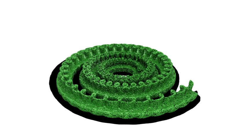
55:2 • Silvia Sellán, Noam Aigerman, and Alec Jacobson
Fig. 2. Subtracting the swept volume of complex brush shapes enables artistic control during 3D carving. 3D model by KellyBC under CC BY-SA 3.0.
Ours Stamping Stamping + grad descent
Input (26M queries) (340M queries) (2137M queries)
0m21s
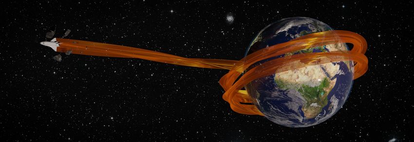
Fig. 3. Our method (green, center left) avoids the stroboscopic artifacts of the stamping at fixed time steps - the only previous work similar in generality
(center right). Stamping and then doing gradient descent in time for each spatial point without our continuation algorithm (right) also presents artifacts
despite incurring a significantly higher computational cost. Scrub to the timestamp listed after any icon in our supplemental video for an animation.
leverages the power of an intermediary implicit representation with- or outside the swept volume. This output sensitivity generalizes to
out inheriting the drawbacks of stamping. Our key insight is that directly contouring interactions with swept volumes such as con-
each point on the surface of the swept volume has an associated structive solid geometry operations (see Fig. 18). With the modern
“timestamp,” corresponding to the moment in which the signed dis- resurgence of implicit modeling (e.g., Adobe Medium, nTopology,
tance to the moving brush is minimized. This timestamp, viewed Dream PS4, Claybook, Neural Implicits [Davies et al. 2021; Park et al.
as a scalar field over R3 , is piecewise continuous. We propose to 2019]), our formulation via implicit functions affords flexibility not
“walk” along the two-dimensional surface of the swept-volume while available with purely explicit methods.
tracking the small changes in timestamp value. By optimizing for We demonstrate the effectiveness and generality of our method
the optimal timestamp (i.e., when the brush was closest) adaptively through a variety of applications spanning 3D modeling, visual
for each point, we ensure an alias-free output. Our approach can be effects, and robotics clearance tasks. We further compare our method
understood as an application of the method of numerical continua- to the state of the art and report superior performance-over-accuracy
tion. Large swathes of 3D space are never even visited, resulting in ratio and surface quality.
an appropriately output-sensitive runtime (scaling with the sweep’s
surface complexity, generally O(n 2 )). 2 WHY YET ANOTHER SWEPT VOLUME METHOD?
Our method is extremely robust, and we have not encountered Computational methods for swept volumes are nearly as old as
any failure case where it has produced an erronous result. Further- computer-aided design itself. Early work focused on accurately
more, our output surfaces consistently match the quality of methods predicting the subtractive modeling processes of CNC milling [Sun-
specialized for specific classes of trajectories (see Figs. 4 & 5). Aside gurtekin and Voelcker 1986; Wang and Wang 1986]. Over the past
from its robustness, the power of our approach is in its generality, decades, a wide variety of techniques for constructing swept vol-
across a few respects: First, the input “3D brush” to our method umes have appeared in the CAD, graphics, and robotics literature,
could be any solid shape representation that admits a continuous with periodic surveys (e.g., [Abdel-Malek et al. 2006]). In this section,
implicit function, such as analytic signed distance functions, approx- we describe how existing methods fall short for critical scenarios.
imate signed distance functions (e.g., arising from constructive solid Since all points on the surface of a solid’s sweep must originate
geometry operations or ShaderToy-esque metric manipulations), from a point on the brush surface, it is natural to consider whether
and robust winding-number [Jacobson et al. 2013] signed distances these points can be explicitly parameterized given a parametric or
from triangle meshes and point clouds. Second, the input trajectory explicit representation of the brush surface. However tempting, ex-
could be any representation of a rigid motion (beyond translations, actly classifying a rigidly moving polyhedron (i.e., piecewise-flat)
screws and splines), but also encompasses articulated rigid bodies involves not just constructing ruled surface patches for each edge
(effectively a union of each body’s sweep) and Minkowski sums and face [Weld and Leu 1990], but also trimming their mutual inter-
(generalizing 1D trajectory curve to a high-dimensional parametric sections to remove components not contributing to the final surface
space). Finally, the output of our basic method is the sweep’s surface, [Blackmore et al. 1999]. Arrangements for planar meshes are already
retrieved via applying dual contouring [Ju et al. 2002] to the sparse daunting, with very recent progress in robust algorithms relying on
set of voxels containing it. This avoids regions of space deep inside exact arithmetic [Zhou et al. 2016] or predicates [Cherchi et al. 2020].
ACM Trans. Graph., Vol. 40, No. 4, Article 55. Publication date: August 2021.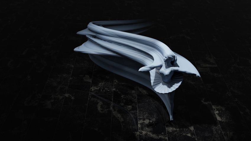
Swept Volumes via Spacetime Numerical Continuation •          55:3

                                                                            [Rossignac et al. 2007] Fig. 1      ours                         ours
                                                                               (screw motions only)        (screw motion)             (non-screw motion)
                                                                            Fig. 5. Our method replicates the main result of Rossignac et al. [2007],
                                                                            while generalizing beyond their restricted class of motions.
 Input       Exact               Ours             Stamping

Fig. 4. Our method indistinguishably reproduces exact translational poly-
hedral sweeps, while stamping exhibits aliasing defects. 3D model by Ceh
Jan under CC BY-SA 3.0.

These are not applicable to the ruled surfaces of a polyhedral sweep.
                                                                                  [Zhang et al. 2009] Fig. 1                         Ours
Pure rational translations can be computed exactly [Zhou et al. 2016]
(see Fig. 4) and screw motions can be well approximated with screw-         Fig. 6. Our results are visually identical to those of Zhang et al. [2009], but
specific analysis [Rossignac et al. 2007] (see Fig. 5), but these do        our method is more general and can work on sweeps theirs cannot.
not generalize to all motions or all classes of brushes. The situation
                                                                            Specifically, if f is a signed distance function then f ⋆ will be an
worsens when compositing sweeping operations with other solid
operations such as Booleans or offsetting [Pavic and Kobbelt 2008].
                                                                            upper bound on the signed distance to the sweep (exact outside,
One option is to approximate surface patches after each operation
                                                                            underestimate inside, cf. [Quílez 2020]).
with point clouds [Peternell et al. 2005], triangle meshes [Abrams
                                                                               Since the input and output are both implicits, swept volumes slide
and Allen 2000], or distance fields [Kim et al. 2004; Zhang et al. 2009],
                                                                            neatly into the larger implicit modeling and rendering frameworks
relying on meshing, ad hoc flood filling or contouring to assemble a
                                                                            [Wyvill et al. 1986]. However, the simplicity of Eq. (1) crumbles
final output surface mesh. These explicit methods accumulate error
                                                                            under scrutiny when turning to implementation. For special combi-
in a hard to control manner.
                                                                            nations of brush functions (e.g., compositions of a small number of
   Campen and Kobbelt [2010] approximate the surface of swept
                                                                            analytic functions) and motion parameterizations (e.g., polynomial
volumes of polyhedra by first discretizing the input motion as
                                                                            splines) root finding can be employed to solve Eq. (1) [Schmidt and
piecewise-linear vertex displacements and then generating a su-
                                                                            Wyvill 2005; Sourin and Pasko 1995]. In contrast, the “R-functions”
perset of candidates from this motion. These must be trimmed and
                                                                            used by Sourin and Pasko [1995] avoid minimization during ag-
                                                                            gregation. While simplifying some derivations, their analogous f ⋆
stitched to form the output. Intersections must be conducted ro-
bustly to ensure a watertight output mesh. Special purpose culling
                                                                            has distorted values away from the zero level-set, precluding direct
rules must be used to avoid the intractable problem of handling all
                                                                            extraction of positive offset surfaces, especially useful in carving
possible intersections. Although code is not available for a direct
                                                                            or robotic clearance problems. Even within their restricted settings,
comparison, we are not confident that this method will be robust
                                                                            numerical root finding is employed at each evaluation point with
in the presence of many intersections, such as in our Fig. 8. Fur-
                                                                            some aspect of global search to avoid local minima. Lacking our
thermore, our algorithm accepts any input rigid motion without
                                                                            continuation-based method, they scale poorly to general inputs and
approximating it, we are not limited to polyhedral inputs and we
                                                                            local minima leave outputs riddled with defects (see Fig. 3).
remove the need for an elaborate post-facto cleanup.
                                                                               One way to sidestep the pitfalls of numerical root-finding is not
   It should be noted that for moving polyhedra, if we insist on a
                                                                            to do it. Instead, one can march at constant time steps, and for each
polygonal mesh as the eventual output, then by design we have to
                                                                            time step fill-in all implicit values at that time step (e.g., on a grid),
accept some approximation error. We should not care whether that
                                                                            a method we refer to as stamping. Stamping lies in direct compar-
error comes from attempting to triangulate exact surface-patches,
                                                                            ison to us, as it is compeletely general (f must only be defined
or contouring an implicit function. We do care that the error is
                                                                            at any point x and moment in time t), and in fact applicable to a
controllable (e.g., by choosing the resolution of the underlying rep-
                                                                            larger set of scenarios (e.g., non-rigid deformations). However, we
resentation), creases are well approximated, and the construction is
                                                                            demonstrate superior surface quality and performance trend. Indeed,
robust and efficient.
                                                                            combined with grids of precomputed f values and adaptive back-
   Compared to explicit representations, a sweeping implicit is sim-
                                                                            ground grids, stamping can be streamlined for memory efficiency
ply stated mathematically. If the input brush solid is the set of points
                                                                            [Von Dziegielewski et al. 2012], but ultimately scales poorly with
x ∈ R3 such that some continuous function f : R3 → R is negative
                                                                            volume, O(n3 ) [Garg et al. 2016; Menon et al. 1994; Schroeder et al.
(f (x) < 0), then the swept volume along some time-parameterized
                                                                            1994]. Furthermore, the choice of the sampling rate is non-trivial:
rigid motion T : [0, 1] → SE(3) is represented as a new implicit func-
                                                                            Sampling too densely in time fills in values deep inside the swept
tion taking the minimum of the brush’s implicit evaluated relative
                                                                            volume as the surface of the brush marches forward. Sampling too
to the motion over time:
                                                                            sparsely leads to temporal aliasing becoming visible (see Fig. 3). This
                     f ⋆ (x) = min f T(t)−1 x .

                                                                      (1)   issue is aggravated by the fact that different points move at different
                              t ∈[0,1]                                      speeds (e.g., through a rotation), hence some spatial regions require

                                                                                   ACM Trans. Graph., Vol. 40, No. 4, Article 55. Publication date: August 2021.
55:4 •   Silvia Sellán, Noam Aigerman, and Alec Jacobson

                                                          time                          If our brush can be represented with an implicit function f , then
              tion         false
            mo         boundary
                                                                       corrections
                                                                                     for any point x in the dark region in Fig. 7 corresponding to the
                                                                                     swept volume there exists some time t such that f (x,t) < 0 (by
                                                                                     slight abuse of notation, we define f (x, t) := f T(t)−1 x ). The true
brush                                                                                and false boundaries are both places where there exists a time t
                          space true boundary                                        such that f (x, t) = 0. Further, at these moments in time necessary
                                                                                     optimality conditions will hold: ∂ f /∂t = 0. However, only for true
Fig. 7. Given an input brush and motion, characteristic points (cf. [Peternell
                                                                                     boundaries will t be the global minimizer (i.e., t = t ⋆ (x), see Eq. (2)).
et al. 2005]) trace true boundaries and false boundaries of the swept volume.           For example, consider a point x
Previous explicit methods pose surface extraction of the swept volume as a           on a red false boundary, correspond-             time
spatial arrangement problem. Instead, we conceptually consider the space-            ing to the time t when f (x, t) = 0.
time hypersurface (codimension one) and trace continuously along the                 Since this point also lies deep in the                  f (x, t) = 0
submanifold (codimension two). Any accidentally explored false boundaries            dark (f < 0) swept volume, there
are corrected when approached from spatially equivalent points.                      must exist some other moment in
                                                                                     time t ⋆ where f reaches its minimal                    f (x, t ) < 0
                                                                                     (negative) value: f (x, t ⋆ ) < 0.                      x
                                                                                        A point x on the true boundary
finer time sampling than others. Frustratingly, the speed of stamp-
                                                                                     curve will reach f = 0 at its globally               time
ing necessary to get an alias-free surface after contouring (e.g., via
                                                                                                     ⋆
                                                                                     optimal time t . There will not ex-
[Lorensen and Cline 1987]) depends on the choice of background
grid resolution. Thus, the number of time samples k in the runtime                   ist any other moment in time where
complexity O(kn 3 ) is effectively dependent on the grid resolution n                f becomes negative. Our method f (x, t ) = 0
(observationally roughly O(n4 )).                                                    seeks to identify all true boundaries
   Contouring static implicit functions invites a similar discussion of              by continuously walking in space-
volumetric (e.g., [Lorensen and Cline 1987]) versus output-sensitive                 time while avoiding overexploring                          x
complexity (e.g., [Bloomenthal 1988; Wyvill et al. 1986]). Bloomen-                  false boundaries. These contours are one dimension less than the
thal casts the tracing of the output surface in the context of the                   full swept volume, so our prospect for performance savings is high.
method of numerical continuation (see, e.g., [Allgower and Georg                        In contrast, naively stamping at dis-
                                                                                                                                     approximate
2003]). The core idea being that once a point x is found such that                   crete moments in time can be understood
f (x) = 0 the necessarily continuous surface must cross grid cells                   as a poor approximation of both the true
neighboring x. Checking only neighbors of previously identified                      and false boundaries. Stamping ignores
surface points avoids visiting the full volume of space. Our method                  the continuity and low dimensionality of
is in essence a continuation method, applied to the minimization                     the spacetime entities and proceeds in
                                                                                     the spatial domain. Even ignoring that                           dense
                                                                                     approximate true boundaries are aliased space
problem (Eq. (1)). However, we apply the continuation not to the
minimum itself, but to its corresponding argmin:
                                                                                     revealing the discretization, stamping litters the interior of the swept
                    t ⋆ (x) = argmin f T(t)−1 x .

                                                                    (2)              volume with candidate false boundaries. Each stamp contributes
                                   t ∈[0,1]                                          new false boundaries that must be trimmed away by subsequent
                                                                                     stamps. As these become dense, performance suffers asymptotically.
  This stems from our core observation: t ⋆ is piecewise-continuous                     Our novel idea is to conduct a self-
over space, enabling our continuation method to propagate argmin                     correcting contouring of the codimen-
values, in turn resulting in a robust and efficient algorithm.                       sion two manifold pre-image of the swept           x
                                                                                     volume boundary in d + 1 spacetime                 t
3    SUBMANIFOLDS IN SPACETIME                                                       rather than directly in d-dimensional
For simplicitiy, let us discuss swept volumes over a 2D example,                     space. Inductively, assuming we have al-
where visualization is simpler. In Fig. 7, we show a prototypical                    ready identified some point (x, t ⋆ ) lying
self-intersecting motion of a solid brush creating a swept 2D “vol-                  on this manifold, we conduct a discrete
ume”. Turning the plane sideways and adding a new dimension                          step-and-project in both space and time to identify a neighboring
for time, we visualize the motion’s spacetime surface. If we imag-                   point also lying on the manifold. Once all points are determined,
ine shining a light from above, then the swept volume is the solid                   we may simply throw away the auxiliary time values. Conducting
shadow captured on the spatial plane. The occluding contours and                     the step-and-project operation requires care, but we will see that
silhouettes represent false and true boundary curves of the swept                    working in spacetime greatly simplifies our algorithm.
volume, respectively. Each curve is composed of continuous parts                        With our crucially different understanding in place, we may now
of the corresponding spacetime curves.                                               describe how we efficiently conduct contouring in spacetime en-
   Our goal will be to walk along just the low-dimensional subman-                   suring a geometrically and topologically valid output. Our two-
ifold of curves on the spacetime surface and output a continuous                     dimensional picture holds analogously when we lift the problem
discretization of the true swept-volume boundaries.

ACM Trans. Graph., Vol. 40, No. 4, Article 55. Publication date: August 2021.
Swept Volumes via Spacetime Numerical Continuation •          55:5

      0m0s

    Input

              Without propagation
                  (fixed seed)           Without propagation (random seed)        With propagation, no backtracking                      Our full algorithm

Fig. 8. An ablation study of our algorithm shows the deterioration in results by omitting the propagation of t ⋆ and using fixed (left) or random (middle) time
seeds, or omitting the correction steps in our algorithm (second to right). Our method (right) recovers the correct surface.

            Ours (100 seeds)      Ours (10 seeds)       Ours (1 seed)
                                                                                     we modify via optimization). On the other hand, the voxels are used
                                                                                     as the “implicit volume element” - we query them and evaluate
                                                                                     each voxel’s 8 vertices’ values to infer whether the zero levelset (the
                                                                                     surface) passes through it or not, and to decide whether to progress
                                                                                     to its neighboring voxels.
      Input     416k voxels visited   422k voxels visited   424k voxels visited         We determine whether the surface passes through a voxel by
                                                                                     checking whether fi⋆ changes sign over the voxel’s 8 vertices –
Fig. 9. Our algorithm is robust to the number of initial seeds in our queue,         since we only sample grid points, vertices rarely if ever land exactly

even in a sweep with self-intersections. 3D model by Jenna Stoeber under             on the surface of the swept volume: i.e., in general f xi , ti⋆ , 0.
CC BY-NC-SA 4.0.
                                                                                     This is not a problem as we merely need to track for which edges
                                                                                     {xi , xj } of the grid does fi⋆ change sign: by continuity, there must
                                                                                     exist some x ∈ {xi , xj } for which f x, t ⋆ (x) = 0 [Lorensen and

to moving solid brushes in 3D, so long as we carefully track co-
dimensionality. Spacetime is now 4D, and our moving brush ex-                        Cline 1987]. We only include voxels that exhibit this sign change in
trudes a hypersurface (3-manifold in 4D spacetime). Its cast shadow                  our output, making it immediately digestible by off-the-shelf sparse
is again 3D (codimension zero) caught in space. Rather than walk                     contouring methods (e.g., [Bloomenthal 1988; Ju et al. 2002]).
along curves in spacetime, we will grow outward along the two-
dimensional (codimension two) submanifold spidering around the                       4.2   Method
spacetime hypersurface.                                                              Our method is in essence a region-growing method reconstructing
                                                                                     the 2D surface in 4D space. Each probe outward from the fron-
4     NUMERICAL CONTINUATION METHOD
                                                                                     tier of the reconstructed surface consists of a discretized spatial
We assume we receive as input an implicit representation f of the                    step (moving on the grid to a neighboring voxel) and a continuous
solid 3D brush (in Section 5, we demonstrate how working with                        optimization for the temporal coordinate, to project it back to t ⋆ .
implicits as input seamlessly enables many other input representa-                   Additional rules stop the region growing at points straying away
tions) and a function T(t) describing the rigid motion of the brush                  from the reconstructed surface, and backtracking to correct wrong-
over a unit duration of some fictitious time. We next describe and                   ful assignments (a minimum is discovered to be local rather than
discuss the continuation method we use to extract the 2-manifold                     global). Fig. 8 shows an ablation study of our algorithm.
embedded in 4D spacetime consisting of the spatial swept volume’s                        For region growing, we keep a (non-priority) queue of voxels to
surface coupled with the extra temporal coordinate t ⋆ .                             visit. Each voxel v on the queue also holds an initial guess of its tem-
                                                                                     poral component tv (to be used as initialization in the optimization
4.1     Voxel grid representation                                                    of the voxel’s vertices’ values). We visit voxels as we pop them from
Our raw output is an implicit representation of the swept volume’s                   the queue. We begin by assuming we have a small number of seed
surface, represented via a sparse voxel grid in 3D. The main param-                  locations (x, t ⋆ ) known to be on the surface of the swept volume
eter of our method is the grid resolution, i.e., the spacing between                 (i.e., f (x, t ⋆ ) = 0).
points on the grid, h ∈ R+ . Internally, we also store a 4th coordinate                  We initialize our queue with the voxels containing the identified
representing t ⋆ , denoted ti⋆ for vertex xi , to distinguish it from the            seed locations lifted to spacetime with corresponding seed’s t ⋆ .
unknown ground truth t ⋆ (xi ). Similarly, we denote the value of the                When popping a voxel v with time value tv from the queue, we
implicit for the vertex as fi⋆ .                                                     visit each of the 8 voxel vertices i to compute its associated ti⋆ , and
   Both the voxels and the vertices of the voxel-grid play a role in                 compare it to any previously-computed value it stores. Consider
our computation. On one hand, the vertices store the computed                        a vertex with spatial position xi . Since we wish to keep it fixed
values (i.e., ti⋆ , fi⋆ ) and can be thought of as semidiscrete objects              to the voxel grid, we move the only degree of freedom available
in 4D. Their location in space is discretized by the step size h (and                — the temporal component — in order to bring the point as close
fixed), while they are endowed with a continuous time value (which                   as possible to the codimension one hypersurface in 4D. We locally

                                                                                            ACM Trans. Graph., Vol. 40, No. 4, Article 55. Publication date: August 2021.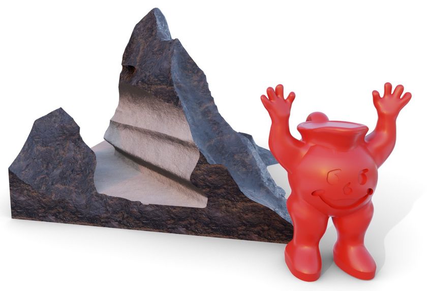
55:6 • Silvia Sellán, Noam Aigerman, and Alec Jacobson
Our algorithm: robust and with better asymptotics Number of queries Runtime (seconds)
10
10 100 1000 100
0 st
100 stamps 1000 stamps Ours 100 am 0s
ps 100 tam
10
9 sta sta ps
mp 100 mp
Ours s 3 s 1
10
8 (1 h( (
3
h(
10 Our
0.6M 6M 2M 2 s
queries 7 (1 h(
10
2
(1 h( 1
6
132q/vert. 10
0.005 0.01 0.05 0.005 0.01 0.05
More hh Less accurate More hh Less accurate
Fig. 11. Our method demonstrates superior performance over stamping,
finer grid
23M 234M 44M typified by results in Fig. 10 using a background grid for implicit querying.
Number of voxels
75q/vert.
Stamping
173M 1730M 190M Ours
100
64q/vert. Exact Solution
10-8 10-6 10-4 10-2
2m07s SDF deviation
Fig. 10. For stamping, the number of fixed-time stamps required for a good Fig. 12. Our algorithm’s produced SDF values are several orders of magni-
result is tied to the spatial resolution: while few stamps may look good for tude more accurate than a similar runtime stamping’s.
coarse spatial resolutions, more and more stamps are required the finer the
resolution gets. Our method doesn’t present this undesirable behaviour. 3D
model by Perry Engel under CC BY-NC 4.0.
Interval basin caching. Voxels and grid vertices may be visited
many times during the queue processing. To avoid re-optimizing
solve this 1D projection problem by conducting gradient descent to the same time values over and over again for the same vertex, we
minimize f (x, t) starting at tv . We simply employ a backtracking take advantage of the 1D nature of the t ⋆ optimziation.
line search [Boyd and Vandenberghe 2004]. Let the time value (the Consider that a vertex has previously started a descent with value
argmin) resulting from gradient descent for this voxel corner be ti . t 0 and converged to the nearest local minimizer t 1 . If we visit this
If this corner has never been visited before, then we set ti⋆ ← ti vertex again and request to start a descent with a value t 2 that lies
in the interval spanned by t 0 and t 1 , then we can skip the numerical
and fi⋆ ← f (xi , ti ). Otherwise, we’ve visited this corner before and
descent and return t 1 immediately as t 2 must lie along the way
need to see whether we have a clash in our hypothesis for t ⋆ , which
down from t 0 to t 1 . In general, a vertex may collect many temporal
we resolve as follows.
intervals. We may merge these using an interval tree as we progress,
If the new implicit value at xi is smaller than the older one,
f (xi , ti ) < fi⋆ , then we’ve identified a correction, meaning the previ-
keeping a map from interval “basins” to associated local minima.
ous value stored was of a strictly-local minimum, and our new value Extracting initial seeds. Our continuation algorithm needs a few
is the new candidate for the global minimum. Hence, we set ti⋆ ← ti initial “seeds”: spacetime points (x, t ⋆ ) such that f (x, t ⋆ ) = 0. Sim-
and fi⋆ ← f (xi , ti ) and add all other voxels incident on this corner ilarly to Peternell et al. [2005], we look for points whose velocity
to the queue endowed with time value ti . Adding the voxels back to and normal vector are orthogonal, a necessary condition for lying
the queue initiates another front propagation that will recursively on the sweep’s surface. We sample time at coarse regular intervals
reevaluate any corner that took part in the front stemming from the (we use 10 intervals for all examples). For each time ti , we draw 100
wrongful local minimum. If the opposite condition holds, i.e., the random points on the brush. For each point, if the orthogonality
old implicit value is smaller than the new one, fi⋆ < f (xi , ti ), then condition is satisfied up to some tolerance (i.e., dot product less than
we are currently tracing a local minimum, so we re-add the current 0.01), we add its corresponding voxel to the queue endowed with
voxel v to the queue with the cached ti⋆ , to have its other corners time ti . Since we are sampling from a superset, we conservatively
recomputed using this time value. compute many of these points (in our examples, 100) and start the
Lastly, if any corner of a voxel was updated, then we consider continuation from all of them. While necessary but not sufficient, we
each edge {i, j} of the voxel for which the signs of fi⋆ and f j⋆ differ. have never encountered an example in which we failed to recover
All other voxels neighboring this edge are added to the queue twice the correct swept volume surface, even when significantly reducing
(once with ti⋆ and once with t j⋆ ). We restate the algorithm above in the number of initial seeds (see Fig. 9). If such example exists, we
pseudocode in the Appendix B. conjecture seeding more aggressively resolves it.
ACM Trans. Graph., Vol. 40, No. 4, Article 55. Publication date: August 2021.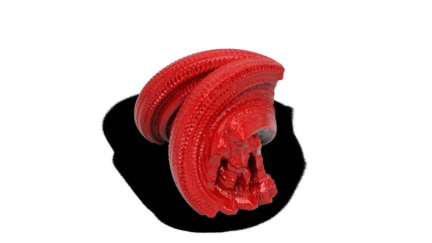
Swept Volumes via Spacetime Numerical Continuation •          55:7

      1m53s
                                                Our output
                                                                                   Square torus

  2D brush

                                                                                   Round torus                                       Our output

Fig. 13. Our method can robustly sweep thin, 2D curves, by sweeping a      Fig. 14. Our method effortlessly sweeps a torus changing shape over time.
small offset from them.

4.3     Discussion
Our method is guaranteed to terminate (queue only grows when
new minima are found and they are finite for a non-fractal f ), and
also guaranteed to output voxel data ensuring a contouring of a
closed surface (no crossing edges may appear on the sparse-voxel
boundary). This is little comfort as the same is true of stamping.
   The major difference for our method is that each update of a grid
vertex is a small finite step from its neighbor’s previously computed
optimal value, leveraging the piecewise continuity of t ⋆ . This is what                                                                            1m57s
enables us to perform significantly fewer queries than stamping. In         Fig. 15. Different geometric brushes produce different artistic profiles.
fact, in Appendix A we show that under sufficient regularity, and
assuming that the implicit function is a signed distance field (as it
                                                                           to stamping (see Fig. 12). In this and all other examples, inputs are
is in most examples in this paper), then given a desired accuracy
                                                                           scaled to fit the unit cube.
tolerance ε of the output, our method requires a number of queries
                                                                              In Fig. 6, we replicate the pièce de résistance from Zhang et al.
which is sublinear, O(log(1/ε)), while stamping requires a number
                                                                           [2009], for which our general method yields the same output. Using
of queries which is linear, O(1/ε).
                                                                           the same brush, we also show a sweep with a more elaborate tra-
   While it is possible to step over a globally optimal value and into
                                                                           jectory. In Fig. 5, we qualitatively match [Rossignac et al. 2007]’s
a nearby local minimum, we do not often observe this. Even if this
                                                                           main result; they are limited to screw trajectories, while we show
does happen once, all other neighbors still have an opportunity to
                                                                           our method’s output on other trajectories not possible with theirs.
send an improvement.
                                                                              In Fig. 3 we show a comparison to the stamping algorithm as well
   Theoretically, a catastrophic sequence of missed global optimums
                                                                           as to an “improved” stamping which, at each grid corner, performs a
could lead to entire patches missing in the output (false positives)
                                                                           fixed number of gradient descent steps on Eq. (1) with equally spaced
or erroneously retained (false negatives). With even mild initial
                                                                           initial guesses. Fast moving or thin components in the input lead to
seeding, we have never witnessed this in all of our experiments.
                                                                           geometric and topological artifacts, while our algorithm recovers
   Compared to stamping, whose worst case behavior spans the
                                                                           those delicate parts perfectly. Furthermore, the number of stamps
entire discretized swept volume, in the worst case, our method traces
                                                                           required to obtain a desirable output is not constant. As we show in
all false boundaries, only to correct them later. We similarly do
                                                                           Fig. 10, an adequate number of stamps at one grid resolution leads
not witness this. In our experiments false boundaries are briefly
                                                                           to staircasing artifacts in the other. Stamping more densely in time
explored but just as quickly corrected. If even a single point on a
                                                                           alleviates that issue at the unacceptable price of a high number of
false boundary component is corrected then the queue acts as a fast
                                                                           queries, significantly increasing the computational cost (see Fig. 11).
breadth first correction for the whole patch.
                                                                           5.2   Geometric modeling via sweeping
5 EXPERIMENTS & RESULTS
                                                                           Our method’s robustness and generality allows exploration of artis-
5.1 Comparisons                                                            tic modeling using sweeps, as shown in Fig. 15. In Fig. 13 we model
We begin with a comparison to various previous techniques for              the horn of a gramophone using a sweep of a 2D curve.
sweeping volume. Fig. 4 shows a comparison of our method to the               Our method is extremely general and opens up the option for
ground truth exact solution, which can be computed in this case            many applications– we can work on any time-evolving signed dis-
of a simple translation along a straight line. Our output is visually      tance field (SDF), as long as it is differentiable with respect to time.
identical, and furthermore has a significantly smaller error compared      Fig. 14 shows an analytic SDF of a torus evolved from the classic

                                                                                  ACM Trans. Graph., Vol. 40, No. 4, Article 55. Publication date: August 2021.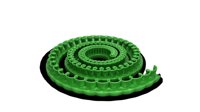
55:8 •    Silvia Sellán, Noam Aigerman, and Alec Jacobson

                                                                                        CSG subtraction

                                                                                                                                s
                                                                                                                        ti   on
                                                                                                                    oca
                                                                                                            er   yl
                                                                                                          Qu                              Our output

                                                                                  Fig. 18. Most of the character’s swept volume does not intersect the moun-
                                                                                  tain. Thanks to our continuation algorithm, we can directly contour the CSG
                                                                                  subtraction without wasting computational time on the irrelevant parts of
Fig. 16. We capture trajectories with a real VR setup and then sweep differ-
                                                                                  the swept volume. Model by Perry Engel under CC BY-NC 4.0.
ent letters’ mesh representations along them.

                                                                                   Input                                            Intersection       2m37s
                                                                          2m45s

                                                                                  Fig. 19. The intersection between the path of a spaceship and a rock for-
                                                                                  mation is computed without necessary computing the swept volume of the
                                                                                  entire path, cutting runtime by a factor of 20. Model by Karl, CC BY-SA 3.0.

                                                                                     In Fig. 19 we show the computed intersection points of a Space
                                                                                  Wizard Vehicle’s path as it is attempting a risky maneuver through a
                                                                                  canyon. Only the red highlighted parts were used in the computation
Fig. 17. We sweep a ballet dancer’s motion, making use of scaling and             of the intersection, speeding up the wall-clock computational time
transparency (the latter, mapped to t ⋆ ) to resemble an artistic motion trail.   by a factor of 15.6×: 344M distance queries (full swept volume)
3D model by Maryam Sadeghi under CC BY-SA 3.0.                                    down to just 24M queries (just intersection). The swept volume on
                                                                                  the left is shown only for trajectory visualization purposes.
                                                                                     In Fig. 20 the sweep of a pendulum is used to design a shape (pink
circular torus at the bottom of the sweep, to a square L 1 -torus at              cylinder) that can rotate while letting the pendulum pass perfectly
the top. The result is a vase with a round bottom and a square top.               pass through it. We perform a change of frame of reference so that
   Similarly, any trajectory can be used as long as it is differentiable          the pink ring is kept fixed and the rest of the world is rotating
with respect to time: In Fig. 16, we interpolated between frames                  around it (on top of the pendulum motion). We then compute the
captured by a virtual reality sculpting application, using Camtull-               subtraction of the pendulum from the pink ring directly.
Rom splines for translation and spherical linear interpolation for                   Of course, CSG operations are useful operations for e.g., modeling,
rotation. Composing the rigid motion with time-varying scaling of                 such as carving a pumpkin using various brushes, as shown in Fig. 2.
the brush is also easy to incorporate, as shown in Fig. 17.
                                                                                  5.4     Path planning
5.3      CSG operations on sweeps                                                 Sweeps can be useful for inferring that total volume that may be
Beyond sweeps, our method can fit within other constructive solid                 potentially occupied by a moving object. In Fig. 21, the joint transfor-
geometry (CSG) operations with sweeps. For example, in Fig. 18 we                 mations of each rigid component are composed to create a complex
subtract a sweep S generated by a moving brush B(t) of the Artifi-                transformation. Our smooth swept volume reveals the space occu-
cially Flavored Drink-Mix Man from an implicitly represented solid                pied by this robotic arm: that is, the areas one should stay clear of
mountain M. Naively, to get a new mountain with a hole punched                    to avoid getting whacked.
through it, N = M \ S, we could run our method to compute S and                      In Fig. 23, we precompute the parking maneuvers of a car, to
then use a standard Boolean operation to perform the subtraction.                 yield a sweep that could guide other vehicles that aim to leave a
However, most of the sweep is far from the mountain and, thus,                    path for the car. In Fig. 24 we compute the Minkowski sum of a 3D
does not affect the resulting N , so there is need to compute it all.             printer’s head with a rectangle, so as to infer the total volume its
Instead, we can turn the order of operations on its head — we define              various motions may take up. To accomplish this, we generalize our
the time-dependent implicit function R(t) = min (−M, B(t)). We                    minimization over 1D time t to the 2D rectangles uv coordinates.
run our continuation method with this implicit function directly.                 While existing methods for exactly computing Minkowski sums of
Fig. 18 shows the total volume actually computed by our in green,                 triangle meshes often lead to expensive pruning and intersection
exhibiting its efficiency. The full red swept volume on the left is               resolving operations (cf. [Campen and Kobbelt 2010; Cherchi et al.
shown only for trajectory visualization purposes.                                 2020]), our algorithm contours the zero level set directly.

ACM Trans. Graph., Vol. 40, No. 4, Article 55. Publication date: August 2021.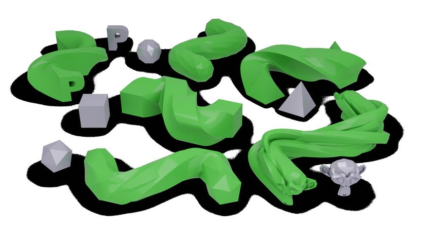
Swept Volumes via Spacetime Numerical Continuation •          55:9

              Input            Swept volume (ours)            CSG result                                             Our output                                 2m50s
       Fig. 20. Changing the frame of reference to that of a fixed wheel allows us to produce this result as a CSG subtraction of a single swept volume.
      2m12s                                                                            2m01s

       Input articulated rigid body        Our output
                                                                                       Input neural implicit                          Our output

Fig. 21. An articulated rigid body can be seen as the union of several solids
                                                                                   Fig. 22. Sweeping a neural network reconstruction of a signed distance field
moving with different trajectories. As such, it fits perfectly into our CSG
                                                                                   obtained via [Davies et al. 2021].
framework and we can compute its swept volume.

5.5     Sweeps on generalized implicit functions                                      Dual contouring the spatial gradient ∂ f ⋆ /∂x (surface normal up
                                                                                   to length) at the identified level-set points xs . In our case,
Our method is readily applicable to other implicit functions. In
                                                                                                          d f⋆     ∂ f ⋆ ∂t ⋆ ∂ f ⋆
Fig. 22, the input is a neural implicit function reconstruction of a                                             =      +                               (3)
chair [Davies et al. 2021]. Likewise, generalized winding number                                           dx       ∂x      ∂x ∂t ⋆
[Barill et al. 2018] enables generating an implicit function from a                Being at a minima ts⋆ , the rightmost term must vanish. Thus it is
point cloud as shown in Fig. 25. As a matter of fact, some of our                  sufficient to compute only the spatial gradient of f evaluated at time
input triangle meshes (like the car in Fig. 23 and the space shuttle               ts⋆ . Occasionally, xs may fall on the medial axis of our brush at ts⋆ ,
in Fig. 1) are non solid models made up of intersecting components,                where f is non-differentiable and does not admit a gradient. In such
but our use of the winding number-signed distance field makes our                  cases, we find finite differencing will be more reliable for computing
algorithm robust to those intersections.                                           these gradients. We observe this rarely for strictly positive level sets,
                                                                                   so our dual contouring uses a numerically tiny offset ε > 0.
5.6     Timing and implementation details
We implemented our method in C++, relying heavily on the library                   6   CONCLUSION
libigl [Jacobson et al. 2018]. We report timings conducted on a 2020               We believe the robust and efficient method for computation of swept
MacBook Pro with a 2.3 GHz Quad-Core Intel Core i7 processor                       volumes introduced in this paper opens up possibilities for future
and 16 GB of memory. The main bottleneck in our algorithm is                       work, such as handling sweeps of non-rigid deformations, or further
the querying of f (x, t) during the gradient descent, consistently                 applications in modeling and path-planning.
taking up over 95% of our runtimes. We share this with the stamping                   We are still unsatisfied with the speed of our method. Even though
algorithm, to which we compare performance-wise in Fig. 10 and                     it surpasses other general techniques in its performance, it is still
Fig. 11. The reduction in asymptotic complexity makes our algorithm                too slow to be used in interactive applications for complex inputs in
faster than stamping at a resolution which produces glaring aliasing               which real time feedback is required. While stamping can work on
artifacts (see Fig. 10, bottom left).                                              a fine grid at real time at the cost of reducing temporal resolution
                                                                                   (thereby creating aliasing), our method is continuous in time. One
5.7     Surface extraction                                                         option to overcome this would be parallelization on the GPU, though
In our results, we use Ju et al.’s dual contouring method for sur-                 less trivial than stamping’s “embarrassingly parallel” nature.
face extraction [2002]. Similar to other surface extraction methods                   Our continuation assumes that the input brush is a solid with
[Bloomenthal 1988; Kobbelt et al. 2001; Lorensen and Cline 1987],                  a well-defined interior and exterior, hence we cannot apply our
it considers each grid edge (x1 , x2 ) crossing the zero level set, with           method directly to infinitely thin sheets, curves or non-orientable
implicit values f 1 < 0 < f 2 and performs a local search to find the              surfaces without introducing a finite offset.
point xs on which the edge crosses the zero level set (f ⋆ (xs ) = 0).                In our experiments, our algorithm never failed to recover the
Dual contouring then uses position and gradient information at                     correct swept volume surface, even when facing pathological trajec-
this point to compute a dual vertex lying in the edge’s neighboring                tories (e.g., Fig. 8), pathologically complex inputs with high genus
(primary) voxel cells. This combines seamlessly with our method:                   (e.g., Fig. 26), very low or high grid size (e.g., Fig. 10) or very low
we keep the argmins t 1⋆ , t 2⋆ and when the binary search asks for the            number of initial queue seeds (e.g., Fig. 9). On the theoretical side,
implicit values f ⋆ of point xs , we perform gradient descent over                 however, we note that we do not have a formal proof of correctness.
f (xs , t), initializing from both t 1⋆ , t 2⋆ and choosing the best result.       We set it as important future work related to formal guarantees on

                                                                                          ACM Trans. Graph., Vol. 40, No. 4, Article 55. Publication date: August 2021.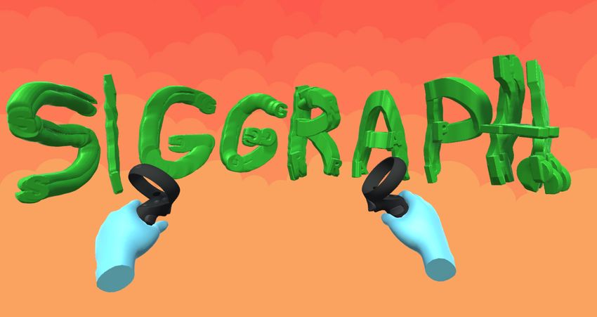
55:10 •   Silvia Sellán, Noam Aigerman, and Alec Jacobson

                                                        2m31s                              2m17s                                    Our output

                                                                                          Input point cloud

Fig. 23. The swept volume by a car performing parking maneuvers could
aid autonomous decision making. Model by W. Mckay, CC BY-NC 4.0.
                                                                                        Fig. 25. Our use of the generalized winding number from [Barill et al. 2018]
                                                                                        to provide a sign to a distance field means we can even compute the “swept
                                                                                        volume” of a point cloud’s isolevel.

                ⊕                                                                          Input

                                                                                                                                   Ours

              Input                Our output
                                                                                        Fig. 26. A stress test of our algorithm containing many intersections. 3D
                                                                                        model by Mariano Mumpower under CC BY-SA 3.0.
Fig. 24. We compute the region of space covered by a 3D printer’s head by
a Minkowski sum with a rectangle to aid design of the printer’s inside.
                                                                                        Gavin Barill, Neil Dickson, Ryan Schmidt, David I.W. Levin, and Alec Jacobson. 2018.
                                                                                            Fast Winding Numbers for Soups and Clouds. ACM Transactions on Graphics (2018).
global root finding methods. A deeper theoretical study of the one-                     Denis Blackmore, Roman Samulyak, and Ming C Leu. 1999. Trimming swept volumes.
dimensional f (x, t) functions and, more critically, a characterization                     Computer-Aided Design 31, 3 (1999), 215–223.
of the discontinuities in the t ⋆ function would not only help in for-                  Jules Bloomenthal. 1988. Polygonization of implicit surfaces. Computer-Aided Geometric
                                                                                            Design (1988).
malizing our method’s robustness, but ideally also in optimizing the                    Stephen Boyd and Lieven Vandenberghe. 2004. Convex Optimization.
choice and number of seeds in our continuation.                                         Marcel Campen and Leif Kobbelt. 2010. Polygonal boundary evaluation of minkowski
                                                                                            sums and swept volumes. In Computer Graphics Forum, Vol. 29. Wiley Online Library.
   Lastly, we believe that many applications concerning time-evolving                   Gianmarco Cherchi, Marco Livesu, Riccardo Scateni, and Marco Attene. 2020. Fast and
implicits and their level sets, such as fluid simulation, can benefit                       Robust Mesh Arrangements Using Floating-Point Arithmetic. ACM Trans. Graph.
from our core observation, of considering the argmin-manifold con-                          (2020).
                                                                                        Thomas Davies, Derek Nowrouzezahrai, and Alec Jacobson. 2021. On the Effectiveness
tinuation - we have just scratched the surface of what is possible                          of Weight-Encoded Neural Implicit 3D Shapes. arXiv:2009.09808 [cs.GR]
with this general technique. To be continued!                                           Akash Garg, Alec Jacobson, and Eitan Grinspun. 2016. Computational Design of
                                                                                            Reconfigurables. ACM Trans. Graph. 35, 4 (2016).
ACKNOWLEDGMENTS
                                                                                        Alec Jacobson, Ladislav Kavan, and Olga Sorkine-Hornung. 2013. Robust Inside-Outside
                                                                                            Segmentation using Generalized Winding Numbers. ACM Transactions on Graphics
This project is funded in part by NSERC Discovery (RGPIN2017–05235,                         (proceedings of ACM SIGGRAPH) 32, 4 (2013), 33:1–33:12.
                                                                                        Alec Jacobson, Daniele Panozzo, et al. 2018. libigl: A simple C++ geometry processing
RGPAS–2017–507938), New Frontiers of Research Fund (NFRFE–201),                             library. http://libigl.github.io/libigl/.
the Ontario Early Research Award program, the Canada Research                           Tao Ju, Frank Losasso, Scott Schaefer, and Joe D. Warren. 2002. Dual contouring of
                                                                                            hermite data. ACM Trans. Graph. 21, 3 (2002), 339–346.
Chairs Program, the Fields Centre for Quantitative Analysis and                         Young J Kim, Gokul Varadhan, Ming C Lin, and Dinesh Manocha. 2004. Fast swept
Modelling and gifts by Adobe Systems, Autodesk and MESH Inc.                                volume approximation of complex polyhedral models. Computer-Aided Design 36,
   We thank Oded Stein, Abhishek Madan and Rahul Arora for their                            11 (2004), 1013–1027.
                                                                                        Leif P Kobbelt, Mario Botsch, Ulrich Schwanecke, and Hans-Peter Seidel. 2001. Feature
help rendering our results; Thomas Davies and David Farrell for                             sensitive surface extraction from volume data. In Proceedings of the 28th annual
providing us the inputs for Fig. 22 and Fig. 16, respectively; Xuan                         conference on Computer graphics and interactive techniques. 57–66.
Dam, John Hancock and all the University of Toronto Department                          William E Lorensen and Harvey E Cline. 1987. Marching cubes: A high resolution 3D
                                                                                            surface construction algorithm. ACM siggraph computer graphics 21, 4 (1987).
of Computer Science research, administrative and maintenance staff                      Jai Menon, Richard J Marisa, and Jovan Zagajac. 1994. More powerful solid modeling
that literally kept our lab running during a very hard year.                                through ray representations. IEEE Computer Graphics and Applications 14, 3 (1994).
                                                                                        Jorge Nocedal and Stephen Wright. 2006. Numerical optimization. Springer.
REFERENCES
                                                                                        Jeong Joon Park, Peter Florence, Julian Straub, Richard A. Newcombe, and Steven
                                                                                            Lovegrove. 2019. DeepSDF: Learning Continuous Signed Distance Functions for
Karim Abdel-Malek, Jingzhou Yang, Denis Blackmore, and Ken Joy. 2006. Swept volumes:        Shape Representation. In Proc. CVPR.
   fundation, perspectives, and applications. International Journal of Shape Modeling   Darko Pavic and Leif Kobbelt. 2008. High-Resolution Volumetric Computation of Offset
   12, 01 (2006), 87–127.                                                                   Surfaces with Feature Preservation. Comput. Graph. Forum (2008).
Steven Abrams and Peter K. Allen. 2000. Computing swept volumes. Comput. Animat.        Martin Peternell, Helmut Pottmann, Tibor Steiner, and Hongkai Zhao. 2005. Swept
   Virtual Worlds (2000).                                                                   volumes. Computer-Aided Design and Applications 2, 5 (2005), 599–608.
Eugene L Allgower and Kurt Georg. 2003. Introduction to numerical continuation          Íñigo Quílez. 2020.        Interior SDFs.     https://www.iquilezles.org/www/articles/
   methods. SIAM.                                                                           interiordistance/interiordistance.htm. Accessed: 2021-05-12.

ACM Trans. Graph., Vol. 40, No. 4, Article 55. Publication date: August 2021.
Swept Volumes via Spacetime Numerical Continuation • 55:11
Jarek Rossignac, Jay J Kim, SC Song, KC Suh, and CB Joung. 2007. Boundary of the least one such i because n > 1/τ ). Now, from the convergence of
volume swept by a free-form solid in screw motion. Computer-Aided Design (2007). a gradient descent with backtracking linesearch (see [Nocedal and
Ryan M. Schmidt and Brian Wyvill. 2005. Generalized sweep templates for implicit
modeling. In Proc. GRAPHITE. 187–196. Wright 2006]) under sufficient regularity conditions,
|t ∗ − i/n| 2
William J Schroeder, William E Lorensen, and Steve Linthicum. 1994. Implicit modeling
1
of swept surfaces and volumes. In Proceedings Visualization’94. IEEE, 40–45. |sd(P, S(t ∗ )) − sd(P, S(t))| ≤ K ≤K m 2 (10)
A. Sourin and A. Pasko. 1995. Function Representation for Sweeping by a Moving Solid. cm c τ
In Proc. Symp. on Solid Modeling and Applications. □
Ugur Sungurtekin and H Voelcker. 1986. Graphical simulation & automatic verification
of NC machining programs. In Proceedings. 1986 IEEE International Conference on
Robotics and Automation, Vol. 3. IEEE, 156–165.
Theorem A.3. Under the regularity conditions described above,
Andreas Von Dziegielewski, Michael Hemmer, and Elmar Schömer. 2012. High quality guaranteeing
conservative surface mesh generation for swept volumes. In 2012 IEEE International sdд t − sdst amp,n ≤ ε (11)
Conference on Robotics and Automation. IEEE, 764–769.
W. P. Wang and K. K. Wang. 1986. Geometric Modeling for Swept Volume of Moving requires O(1/ε) evaluations of sd(P, S(t)), while guaranteeing
Solids. IEEE Computer Graphics and Applications 6, 12 (1986).
John D. Weld and Ming C. Leu. 1990. Geometric Representation of Swept Volumes with sdд t − sdour s,n,m ≤ ε (12)
Application to Polyhedral Objects. Int. J. Robotics Res. (1990).
Geoff Wyvill, Craig McPheeters, and Brian Wyvill. 1986. Soft objects. In Advanced requires O(log(1/ε)) evaluations of sd(P, S(t)).
Computer Graphics. Springer, 113–128.
Xinyu Zhang, Young J Kim, and Dinesh Manocha. 2009. Reliable sweeps. In 2009 Proof. The first statement is a direct consequence of Lemma A.1,
SIAM/ACM joint conference on geometric and physical modeling. 373–378. while the second comes from Lemma A.2, making n = ⌈1/τ ⌉ and
Qingnan Zhou, Eitan Grinspun, Denis Zorin, and Alec Jacobson. 2016. Mesh Arrange-
ments for Solid Geometry. ACM Trans. Graph. (2016).
m = log(K/ετ 2 ), leading to
1 K
logc 2 (13)
A THEORETICAL CONVERGENCE τ ετ
In what follows, assume a shape S is being swept along a trajectory function evaluations. □
S(t) with 0 ≤ t ≤ 1 whose velocity and acceleration are bounded in
B PSEUDOCODE
norm from above by vb , ab . Let sd(P, S(t)) be the SDF of S(t) mea-
sured at point P, and further assume the SDF is twice-differentiable
with respect to t for all P. Let Algorithm 1: argmin Continuation Method
sdдt (P) = min sd(P, S(t)) (4) let fi , ti be the stored implicit and time values at corner i
0≤t ≤1
Insert voxel and time seeds into Q
be the groundtruth swept volume SDF, while Q is not empty do
sdst amp,n (P) = min sd(P, S(i/n)) (5) v, tv ← pop voxel and time from Q
i ∈ {0, ...,n }
for each corner i of the eight corners of v do
be the stamping algorithm SDF with n stamps and fi , ti ← backtracking gradient descent from tv at xi
sdour s,n,m (P) = min дm (sd(P, S(i/n))) (6) if first time seeing i then
i ∈ {0, ...,n } fi⋆ , ti⋆ ← fi , ti
be a conservative version of our algorithm which samples uniformly else if fi < fi⋆ then
in time and then carries out m iterations of backtracking gradient fi⋆ , ti⋆ ← fi , ti
descen (дm ) t for each of the samples. Also, let τ be the length of for each other voxel n incident on i do
the minimum interval in which sd(P, S(t)) is strongly convex and push (n, ti ) onto Q
Lipschitz-smooth as a function of t.
else
Lemma A.1. In the above conditions, push (v, ti⋆ ) onto Q
v
sdдt − sdst amp,n ∞ ≤ b (7) if any corner was updated then
2n
for each edge {i, j} of the twelve corners of v do
Proof. Let P be a point in space and t ∗ = argmin sd(P, S(t)). Let if signs of fi⋆ and f j⋆ differ then
i be the closest uniform timestep such that |i/n − t ∗ | ≤ 1/2n. Then, for each other voxel n incident on {i, j} do
|sd(P, S(i/n)) − sd(P, S(t ∗ ))| ≤ vb
1
. (8) push (n, ti⋆ ) onto Q
2n push (n, t j⋆ ) onto Q
□
Lemma A.2. In the above conditions, if n > 1/τ , there exists a
constant K ∈ R and a c > 1 such that for big enough m,
1
sdдt − sdour s,n,m ∞ ≤ K 2 m (9)
τ c
Proof. Let P be a point in space and t ∗ = argmin sd(P, S(t)).
Let i/n one of the uniform sample which falls on the interval on
which the function is convex and which contains t ∗ (there is at
ACM Trans. Graph., Vol. 40, No. 4, Article 55. Publication date: August 2021.You can also read