Estimation of Stability Parameters for Wide Body Aircraft Using Computational Techniques
←
→
Page content transcription
If your browser does not render page correctly, please read the page content below
applied
              sciences
Article
Estimation of Stability Parameters for Wide Body Aircraft
Using Computational Techniques
Muhammad Ahmad *,† , Zukhruf Liaqat Hussain † , Syed Irtiza Ali Shah and Taimur Ali Shams

                                          Department of Aerospace Engineering, College of Aeronautical Engineering, National University of Sciences
                                          and Technology, Islamabad 44000, Pakistan; zliaquat.ms13ae@student.nust.edu.pk (Z.L.H.);
                                          irtiza_shah@gatech.edu (S.I.A.S.); taimur.shams@cae.nust.edu.pk (T.A.S.)
                                          * Correspondence: mahmad.ms13ae@student.nust.edu.pk
                                          † These authors contributed equally to this work.

                                          Abstract: In this paper, we present the procedure of estimating the aerodynamic coefficients for a
                                          commercial aviation aircraft from geometric parameters at low-cruise-flight conditions using US
                                          DATCOM (United States Data Compendium) and XFLR software. The purpose of this research
                                          was to compare the stability parameters from both pieces of software to determine the efficacy of
                                          software solution for a wide-body aircraft at the stated flight conditions. During the initial phase
                                          of this project, the geometric parameters were acquired from established literature. In the next
                                          phase, stability and control coefficients of the aircraft were estimated using both pieces of software in
                                          parallel. Results obtained from both pieces of software were compared for any differences and the
                                          both pieces of software were validated with analytical correlations as presented in literature. The
                                          plots of various parameters with variations of the angle of attack or control surface deflection have
                                also been obtained and presented. The differences between the software solutions and the analytical

                                          results can be associated with approximations of techniques used in software (the vortex lattice
Citation: Ahmad, M.; Hussain, Z.L.;       method is the background theory used in both DATCOM and XFLR). Additionally, from the results, it
Shah, S.I.A.; Shams, T.A. Estimation      can be concluded that XFLR is more reliable than DATCOM for longitudinal, directional, and lateral
of Stability Parameters for Wide Body     stability/control coefficients. Analyses of a Boeing 747-200 (a wide-body commercial airliner) in
Aircraft Using Computational              DATCOM and XFLR for complete stability/control analysis including all modes in the longitudinal
Techniques. Appl. Sci. 2021, 11, 2087.
                                          and lateral directions have been presented. DATCOM already has a sample analysis of a previous
https://doi.org/10.3390/
                                          version of the Boeing 737; however, the Boeing 747-200 is much larger than the former, and complete
app11052087
                                          analysis was, therefore, felt necessary to study its aerodynamics characteristics. Furthermore, in this
                                          research, it was concluded that XFLR is more reliable for various categories of aircraft alike in terms
Academic Editor: Jens Sørensen
                                          of general stability and control coefficients, and hence many aircraft can be dependably modeled and
Received: 14 December 2020                analyzed in this software.
Accepted: 17 February 2021
Published: 26 February 2021               Keywords: aerodynamic coefficients; Boeing; DATCOM; stability and control; XFLR

Publisher’s Note: MDPI stays neutral
with regard to jurisdictional claims in
published maps and institutional affil-   1. Introduction
iations.                                       The Boeing 747-200 is a long-range, wide-body, large aircraft designed and developed
                                          by Boeing, a commercial airplane company in the USA. It is powered by a high-bypass
                                          turbofan engine developed by Pratt and Whitney. Some different variants also have GE-
                                          CF6 engines, and original variants have Rolls-Royce RB211 engines. It has a pronounced
Copyright: c 2021 by the authors.         wing sweep, allowing a cruise Mach number of 0.90. The 747-200B was the basic passenger
Licensee MDPI, Basel, Switzerland.        version of its series with increased fuel capacity and more powerful engines. General
This article is an open access article    specifications of the Boeing 747-200 are given in Table 1.
distributed under the terms and
conditions of the Creative Commons
Attribution (CC BY) license (https://
creativecommons.org/licenses/by/
4.0/).

Appl. Sci. 2021, 11, 2087. https://doi.org/10.3390/app11052087                                              https://www.mdpi.com/journal/applsci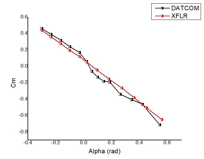
Appl. Sci. 2021, 11, 2087                                                                                         2 of 25

                            Table 1. General specifications of the BOEING 747-200 aircraft [1].

                                    S No.                         Specification                      Value
                                       1                   Maximum takeoff weight                  833,000 lbs
                                       2                         Total length                      231 ft 10 in
                                       3                        Cabin width                          239.5 in
                                       4                     Vertical tail height                   63 ft 5 in
                                       5                        Fuel capacity                     53,985 US gal
                                       6                            Thrust                          54,750 lbf
                                       7                            Range                           6560 nm
                                       8                           Take off                          10,900 ft
                                       9                       Type of engine                         JT9D-7

                                 Flow field characteristics can be obtained by applying various aerodynamic flow
                            models. Navier–Stokes (NS) equations are the most accurate flow models that describe
                            viscous, rotational, and compressible flows. These are based on the Eulerian approach and
                            primarily describe the momentum equation. The mass and energy equations are defined
                            using additional relations to solve NS equations [2].
                                 Based on the accuracy and vast applications, NS equations are used in different forms,
                            such as direct numerical solution (DNS), large eddy simulation (LES), unsteady Reynolds-
                            averaged Navier–Stokes (URANS), Reynolds-averaged Navier–Stokes (RANS), thin-layer
                            Navier–Stokes (TLNS), and turbulence modeling (TM) [3]. Boundary-layer equations are
                            based on the concept that at large Reynolds numbers, the viscous effects are limited to a
                            thin region of flow adjacent to the body surface. BL equations are found by dropping the
                            viscous diffusion terms from Navier–Stokes equations because they have little contribution
                            to the solution. The pressure is assumed to be constant along the length in BL models [4].
                            Euler equations are the conservation laws assuming inviscid flow. The continuity equations
                            do not change; however, energy relations may vary according to the flow characteristics.
                            The assumption of inviscid flow does not limit the applicability of these equations. More-
                            over, outside the boundary layer, this assumption is also feasible for the flow properties.
                            Modeling flow can be further simplified if the flow is assumed to be irrotational (zero
                            vorticity) [5]. The full potential model combines all the conservation laws (continuity,
                            momentum, and energy equations) [6]. Linearized potential equations are developed by
                            decomposing the velocity into an unperturbed component and a perturbed component,
                            which helps one to solve the non-linearity. Prandtl–Gluert’s relation applies to the flows
                            outside the transonic and hypersonic regimes [7]. For an incompressible flow, the Laplace
                            equation in full potential form is reduced to partial differential equations. The Laplace
                            equation has linearized behavior and has an exact solution. The discretization form of this
                            equation is not required, and hence numerical errors do not exist [8]. Empirical methods
                            do not model the flow; however, these can be used for the estimation of aerodynamic
                            performance [9]. Estimations of lift, drag, and aerodynamic efficiency can be performed
                            by using empirical methods. These methods are further used for stability and control
                            derivatives of the complete aircraft, for instance, in US DATCOM (United States Data
                            Compendium). The evolution of various aerodynamic flow models is described in the flow
                            chart shown in Figure 1.
Appl. Sci. 2021, 11, 2087                                                                                            3 of 25

                            Figure 1. The evolution of aerodynamic flow models [3,10,11].

                                  Aerodynamic coefficients can be estimated using experimental and computational
                            techniques. There are various computational techniques available, e.g., DATCOM, XFLR,
                            TORNADO, AVL, PANAIR, and ANSYS. Each technique has its limitations that restrict
                            its areas of application. TORNADO is a program based on potential flow theory that
                            incorporates the vortex lattice method as its background theory. The wake from lifting
                            surfaces creates vortices and TORNADO captures these effects through horse-shoe or
                            horse-sling arrangements. This program determines the first-order derivatives using a
                            central-difference calculation with the help of a pre-selected state and a disturbed state. The
                            results obtained are accurate only for small rotations or small angles of attack. Moreover,
                            compressibility effects are also not catered to in TORNADO; hence, high Mach number
                            situations cannot be handled accurately [12].
                                  Athena Vortex Lattice (AVL) was developed for the MIT Athena TODOR aero software
                            collection. AVL also solves potential flow through the vortex lattice method. It assumes
                            quasi-steady flow and the compressibility effects are provided through the Prandtl–Gluert
                            model. This program was designed for thin airfoils, small angles of attack, and sideslip.
                            Since slender body analysis is not accurate, it is often suggested to leave fuselage out of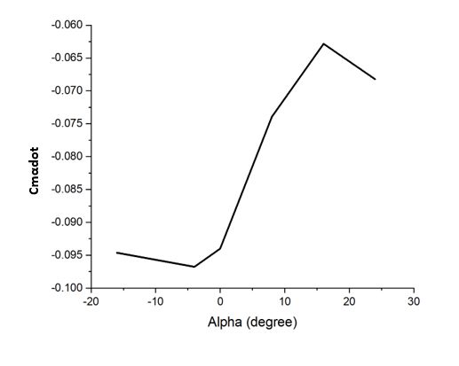
Appl. Sci. 2021, 11, 2087                                                                                           4 of 25

                            the analysis in AVL [13]. Panel Aerodynamics (PANAIR) is a program that uses a higher-
                            order panel method to predict boundary value problems using Prandtl–Gluert relations. It
                            provides a higher-order modeling capability in subsonic and supersonic regions. PANAIR
                            revolutionized the supersonic surface modeling in contrast to average surface meshes. The
                            higher-order panel method yields accurate velocity distributions. PANAIR cannot predict
                            flow dominated by viscous and transonic flow effects. Automatic wake determination
                            through PANAIR is also not accurate. Moreover, for configurations with different total
                            pressures, this program cannot accurately predict the flow characteristics [14]. FLUENT
                            and CFX are two modules of ANSYS. FLUENT employs a cell-centered method and CFX
                            works on a vertex-centered approach. This software can handle different types of meshing
                            operations. such as polyhedral and cut cell meshing (in the case of FLUENT) and tetra and
                            hexa mesh topologies (in the case of CFX). ANSYS is an excellent tool to determine stability
                            and control characteristics, but it takes a long time and has a complex mesh generation
                            process. For industry, it is an ideal tool, since its accuracy and precision is comparable to
                            wind tunnel testing.
                                  Aerodynamic Model Builder (AMB) is a module dedicated to stability and control
                            of the aircraft. It is used to estimate the aerodynamic forces and moments [15,16]. Unlike
                            DATCOM, aerodynamic analysis can be performed in TORNADO software. Moreover,
                            compressible and non-viscous flows can be solved using EDGE (CFD solver) for an irregu-
                            larly structured tetrahedral mesh produced by the mesh generators SUMO and Tetgen [15].
                            The feasibility of hypersonic flight is highly dependent on the controller’s design. Due to
                            extreme flow conditions, it is a challenge to develop a design for a large flight envelope
                            and strong interactions between propulsion and structural systems [17,18]. However, the
                            control-oriented model, truth model, wing-cone model, curve-fitted model, and re-entry
                            motion are few techniques with which to take up this challenge [17]. The aerodynamic
                            stall is an important phenomenon while determining the stability and control character-
                            istics [19,20]. Beyond this point, non-linearities and instabilities appear in the flow, and
                            analysis models must be accurate to comment on the complicated flow field. Bifurcation
                            analysis is a tool that discusses the effect of unknown pitch damping dynamics when the
                            aircraft is under a deep-stall transition [21]. Another approach to study the instability ef-
                            fects in time-domain methods is the recursive least squares. The technique uses a recursive
                            formulation to account for residuals, encountered during estimation of aircraft parame-
                            ters [22,23]. The flow phenomenon over the control surfaces or wing may undergo large
                            variations; therefore, precise simulations are required to obtain accurate results [20,24]. In
                            order to predict the responses for unsteady and nonlinear flight envelopes in high maneu-
                            vering operations, extensions to aerodynamic models need to be incorporated [25]. Due
                            to extreme flight conditions, civil or military aircraft may cross normal operating limits.
                            Therefore, prevention or recovery methods are also required to be incorporated in the
                            aerodynamic model [26]. The development of extensive aerodynamic modeling techniques
                            can fulfill these requirements [19]. Information about identification of model can also be
                            obtained from dynamic test methods [27]. The modeling of rotorcraft aerodynamic inter-
                            ference has proven to be a challenging problem due to the complex flow-field interactions
                            between the rotors and other aircraft subsystems. An effective and efficient aerodynamic
                            simulation tool was proposed by combining a Lagrangian solver [21,28]. Data obtained
                            from a quick accesses recorder (QAR) is another efficient way to determine the effects of
                            extreme weather conditions [22,29].
                                  Bryan introduced the theory of aerodynamic derivatives in 1911, and it has remained
                            unchanged as the standard pattern for the interpretation of the aerodynamic loads in
                            equations of motion (EOMs). Aerodynamic forces and moments are assumed to be the
                            functions of control angles, disturbance velocity, and rates of control angles. At low angles
                            of attack (AoA) and in slow-moving airplanes, aerodynamic loads can be easily modeled
                            by using static derivatives. However, at high AoA, dynamic derivatives can greatly affect
                            the stability characteristics [30]. The variation in the stability derivative can be taken
                            into account by adding the non-linear terms along with extensions in the range of flight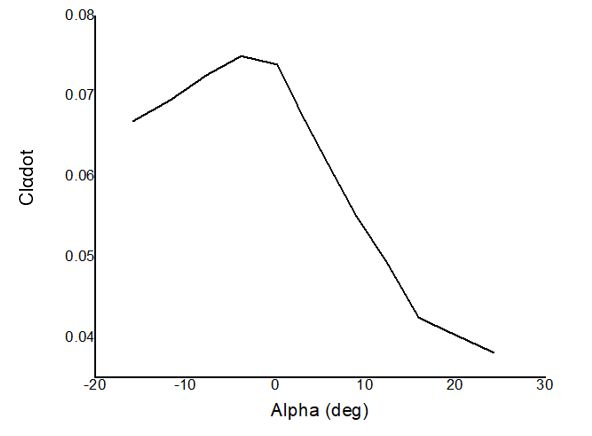
Appl. Sci. 2021, 11, 2087                                                                                            5 of 25

                            conditions [31]. Grauer and Morelli [32] developed a procedure to determine the single
                            generic global aerodynamic model structure that could be applicable to various aircraft.
                            The analysis was carried out by applying multivariate-orthogonal-function modeling on
                            wind-tunnel aerodynamic databases of different aircraft over a wide range of angles, rates,
                            and deflections of control surfaces.Drela et al. [33] investigated the aerodynamic benefit
                            from ingestion of boundary layer of a transport aircraft. The power balance method was
                            developed based upon the mechanical power required and streamwise forces acting on
                            the aircraft. The results showed an increase in efficiency of up to 9% at low cruise power
                            conditions. Grauer and Morelli [34] developed a generic nonlinear aerodynamic model
                            based upon multivariate orthogonal function. The model accurately predicted the global
                            and local dynamic behavior and trim solutions over a range of large amplitude excitations.
                            Triet et al. [35] and Nguyen et al. [36] performed aerodynamic analysis of an aircraft wing
                            using computational fluid dynamics. The variation of velocity and pressure distribution
                            on the wing was captured by using ANSYS Fluent package. The coefficients of lift and
                            drag were estimated based upon data obtained at different boundary conditions. Vecchia
                            and Nicolosi [37] provided the guidelines in the design and optimization of transport
                            aircraft. MATLAB algorithm was developed to determine the aerodynamic coefficients.
                            The panel code solver was used to optimize the geometrical shapes. The procedure helped
                            to import and modify geometries by interpolation of curves and surfaces.Nicolosi et al. [38]
                            presented a method to determine the aerodynamic performance of aircraft fuselage. During
                            the study, the contribution of the fuselage to overall stability and its interactions with the
                            wings and tail were investigated. Numerical simulations were carried out based upon CFD
                            techniques and aerodynamic coefficients were estimated. Ammar et al. [15] performed the
                            stability analysis of a blended-wing-body aircraft. The static and dynamic stability and
                            flying quality analysis was carried out in a flight envelope by applying aircraft synthesis
                            and integrated optimization methods. The flight envelope was created and the TORNADO
                            program was used to estimate the aerodynamic coefficients of aircraft. Rizzi [39] presented
                            an overview of the simulated stability and control system of an aircraft. Flying and handling
                            qualities were determined using integrated optimization techniques. Lu [40] investigated
                            the dynamic stability and control characteristics of a tilt-rotor aircraft using mathematical
                            nonlinear flight dynamics techniques. The damping coefficients in longitudinal and lateral
                            modes were estimated and their effects on overall stability characteristics were analyzed.
                                  The geometric parameters along with flight conditions are the basic and most impor-
                            tant requirements for modeling the aircraft in any software. The data of a Boeing 747-200
                            are readily available in online sources to be used as the foundations of modeling and
                            analysis of the aircraft. The geometric parameters along with control surface clearances
                            were acquired from established literature and reliable online sources [41]. Based upon
                            theoretical knowledge such as the vortex latex method (VLM), source code was generated
                            in both computer programs. For modeling of aircraft to acquire stability and control deriva-
                            tives, design flight conditions were used. Analytical results available in the literature for
                            low-cruise-flight conditions were selected as a benchmark. Figure 2 shows the flow chart of
                            the methodology adopted during the project. The parameters in both software applications
                            were derived from basic equations of motion (Equations (1)–(6)) for an aircraft (six degrees
                            of freedom system) readily available in the literature [1,42].
                                  Force equations:
                                                                         du
                                                                Fx = M (     + qw − rv)                                 (1)
                                                                          dt
                                                                         dv
                                                                Fy = M (     + ru − pw)                                 (2)
                                                                         dt
                                                                         dw
                                                                Fz = M (     + pv − qu)                                 (3)
                                                                          dt
                            Moment equations:
                                                              dp       dr
                                                       l = Ix     − Ixz + qr ( Iz − Iy ) − Ixz pq                       (4)
                                                              dt       dt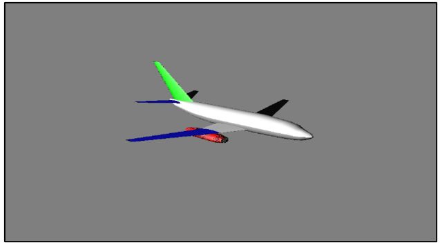
Appl. Sci. 2021, 11, 2087                                                                                            6 of 25

                                                                dq
                                                       m = Iy       + Ixz ( p2 − r2 ) + pr ( Ix − Iz )                   (5)
                                                                dt
                                                               dr       dp
                                                       n = Iz − Ixz          + pq( Iy − Ix ) + Ixz qr                    (6)
                                                               dt       dt
                            where l, m, and n represent the rolling, pitching, and yawing moments. Fx , Fy , and Fz
                            represent the resultant forces in longitudinal, lateral, and vertical axes, respectively. The
                            symbols M and t represent the mass of the body and the time domain, respectively. The
                            symbols u, v, and w represent the axial, side, and normal velocity components, respectively.
                            The symbols p, q, and r represent the roll, pitch, and yaw rates, respectively. Ix , Iy , and Iz
                            represent the moment of inertia components in x, y, and z-axes. Iyz , Izx , and Ixy represent
                            the products of inertia in roll, pitch, and yaw axes.

                            Figure 2. Methodology adopted during the research.
Appl. Sci. 2021, 11, 2087 7 of 25
The equations of motion are derived for a particular axis system specific to the aircraft.
Equations for aerodynamic, gravitational, and propulsive are derived using Newton’s
equations of motion while applying Euler angle corrections to make the equations consis-
tent in one frame of reference. Small-angle approximation and steady flight conditions are
used to linearize the equations with the assumption that small perturbations occur in the
motion of an aircraft during steady flight. This assumption holds good for the theoretical
determination of stability for the small-amplitude motion of aircraft. Once employed,
forces/moments in x, y, and z-directions are computed and observation is the coupling of
lateral and directional motion. The stability and control of an aircraft can be troublesome
if things are discussed in theoretical form but a representation using stability and control
coefficients makes life easier. After the development of complete linearized equations of
motion, Taylor’s series expansion is used to determine the relations of the rates of change
of stability parameters. The expressions of stability/control coefficients and derivatives
are used in software solutions to run the simulations of modeled aircraft. The results are
obtained using visual tools along with insights into the aerodynamic behavior of aircraft
during motion.
In the present research, stability parameters for wide-body aircraft have been estimated
using computational techniques. The comparison of statistical software (DATCOM) with
a computational technique (XFLR) for a wide-body Boeing 747-200 is also presented.
Although these software programs have been tested and evaluated multiple times, a one-
to-one comparison for a Boeing 747-200 is the first of its kind. Results obtained from US
DATCOM and XFLR software were compared for any differences and the they were also
validated with analytical correlations presented in the literature. The material covered in
the different sections is as follows.
In the second section, a brief overview of the US DATCOM algorithm, its applications,
and its working principle to determine the stability and control coefficients have been
discussed. Aerodynamic coefficients of a wide-body airplane have been estimated at given
flight conditions. The variations of lift, drag, and moment coefficients have been obtained
at various angle of attack. Moreover, longitudinal and lateral aerodynamic coefficients
have also be acquired at different angles of attack and control surface deflections. In the
third section, the XFLR algorithm to determine the stability and control analyses of an
aircraft has been elaborated. The various applications and limitations of XFLR in aircraft
design and analysis have also been discussed. In order to estimate the aerodynamic
coefficients of Boeing 747-200 aircraft, the elements of the design process, including direct
foil analysis, and wing and body design and analysis have been elaborated. The results
of lift, drag, and moment coefficients have been acquired at different angles of attack
and they have been plotted. Moreover, to check the stability conditions, eigenvalues
for longitudinal stability (short period and Phugoid) and lateral stability (spiral, roll,
and Dutch roll) modes have also been evaluated. In the fourth section, results obtained
from both the commercial packages are presented in terms of dimensionless aerodynamic
coefficients. Results obtained at low-cruise-flight conditions have been compared with the
analytical results available in the literature. The comparative analysis shows that results
obtained from computational techniques are quite close to each other and to the analytical
results. The comparison of longitudinal and lateral coefficients obtained from both pieces
of software with the results available in the literature is summarized in Appendix A. In the
fifth section, analysis and discussion of the results obtained from both pieces of software
have been given. Aerodynamic coefficients having a great influence on the accuracy
of the results for the validation of the codes are also presented. Moreover, a graphical
representation of aerodynamic coefficients at different angles of attack have also been
added. In the sixth section, the conclusions have been drawn based on a comparison
of results and computational analysis. The analysis provides meaningful results for the
estimation of longitudinal stability and control derivatives from the knowledge of aircraft
geometrical parameters and given flight conditions. In order to improve the source codeAppl. Sci. 2021, 11, 2087 8 of 25
by exploring some advanced features, a few recommendations have also been added in
that section.
2. US DATCOM
DATCOM is a computer algorithm that is used to estimate the aerodynamic prop-
erties, i.e., stability and control coefficients of fixed-wing aircraft either by extrapolation
or interpolation of information available in a database [43]. The computer program was
modified into commercial software that has been extensively used in academia as one of
the reliable tools for the stability and control of an aircraft. The software now is in the
public domain and has been replaced in the aerospace industry by newer computational
analysis options [44,45]. It is a combination of theoretical and experimental procedures
that are required to analyze aerodynamic stability and control parameters. DATCOM
can be used for the autonomous design of the flight control system for a fixed/blended
wing aircraft [46]. Aerodynamic parameters are generally obtained from wind tunnel
testing, computational fluid dynamics, or flight tests; however, dimensionless aerodynamic
stability (static/dynamic) derivatives can be directly estimated using DATCOM [47]. The
inputs required in DATCOM are only physical dimensions and flight conditions, but the
output can be varied according to the requirements. Not only can the coefficients of the
entire aircraft be obtained, but individual surfaces or a combination can also be produced
as an output. Additional output configurations include wing, horizontal tail, wing–tail,
and wing–fuselage–horizontal tail configurations. In DATCOM, forward lift surfaces are
always treated as wing and the aft lift surface is considered as a tail [48]. The analysis gives
meaningful results for the estimation of a complete set of longitudinal stability and control
coefficients for lifting, stability, and control surfaces. Aircraft model simulation can also
be obtained to visually check the various surfaces. Figure 3 shows the Boeing 737 model
obtained from DATCOM based upon geometric parameters. The output can further be
utilized to evaluate the flight dynamics characteristics. Aircraft control surface deflections
and aerodynamic data at various Mach number regimes can also be computed [49].
Figure 3. Boeing 737 model, as prepared using US DATCOM in this research.
The characteristics based on body aerodynamics and subsonic longitudinal data can
be obtained at different Mach numbers for rotational and cambered bodies having arbitrary
cross-sectional areas [50]. Moreover, the trim output can also be computed by the manipu-
lation of stability and control characteristics. The trim mode includes a horizontal tail or
wing coupled with a trim control mechanism and longitudinal aerodynamic characteristics,
and deflection angles required to trim are obtained as outputs. Some special control proce-
dures, i.e., hypersonic flap methods related to controllability and stability for high-speed
operating devices, are also incorporated in DATCOM. The initial sizing procedure of 2D
transverse jet controls for an aft-end located nozzle operating at a high Mach number
can be obtained from this technique. Moreover, the interaction of the local flow field and
transverse jet can also be evaluated. The output from DATCOM can be imported into
MATLAB through the MathWorks Aerospace Toolbox where static and dynamic stabilityAppl. Sci. 2021, 11, 2087 9 of 25
and control derivatives can be stored in arrays that can be further used in the Simulink
block for stability analysis.
2.1. Aerodynamic Coefficients Estimation Using US DATCOM
DATCOM treats various high lift devices, including plain, single/double slotted jet
flaps; leading-edge flaps; and control devices, such as spoilers and typical wing–body–tail
configuration with controlled effectiveness. The software application is well-designed
for the conventional aircraft configurations [51]. The characteristics including lateral,
longitudinal, and directional stability obtained from DATCOM are in the stability axis
system. For specific configurations and Mach number regimes, coefficients, e.g., Clβ, Cmα,
Cnβ, CLα, CL, Cm, and CD, can be obtained from the DATCOM output file. Additionally,
parameters such as lift, roll, moment, normal dynamic derivatives, side-force for the angle
of attack, and angular rates can also be computed [48]. Flight conditions are defined in
DATCOM based on Reynolds number and Mach number data. This condition can be
satisfied by defining velocity, altitude, temperature, and pressure along with the requisite
Reynolds number and Mach number. In the present study, aerodynamic coefficients of the
Boeing 747-200 airplane at low-cruise-flight conditions (M = 0.5, Alt = 20,000 ft, and α = 6.8
deg) were estimated.
2.2. Geometric Parameters
Geometric parameters required for analysis (estimation of aerodynamic coefficients)
were obtained from the established literature and reliable online sources. Some of those
parameters are given in Table 2.
Table 2. Geometric parameters of BOEING 747-200 aircraft [52].
S No. Geometric Parameter Symbol Value
1 Reference area S 5500 ft2
2 MAC C 27.3 ft
3 Wingspan b 196 ft
4 Mach No (cruise) M 0.9
5 True airspeed V 871 ft/s
6 Dynamic pressure P 222.8 Psi
7 CoG location Xcg/C 0.25
8 Angle of attack (cruise) α 2.4 deg
9 Weight W 636,636 lbs
10 Moment of inertia Ixx 1.82 × 10⁷ slug-ft2
11 Moment of inertia Iyy 3.31 × 10⁷ slug-ft2
12 Moment of inertia Izz 4.97 × 10⁷ slug-ft2
13 Inertia moment product Ixz 9.7 × 10⁵ slug-ft2
14 Fuselage length L 225.17 ft
15 Wing sweep angle ∧ 37.5 deg
16 Aspect Ratio AR 7
The scaled-down model drawings of the Boeing 747-200 airplane with dimensional
parameters and horizontal/vertical clearances obtained are shown in Figure 4. Based upon
geometric parameters and horizontal/vertical clearances, source code was generated in
DATCOM by applying VLM theory.
2.3. US DATCOM Results
After the generation of source code, stability/control analysis was carried out, and
results from US DATCOM at low-cruise-flight conditions with variations of the angle of
attack and control deflection were obtained. The variation of different stability/control
coefficients in both longitudinal and lateral modes can be seen with the angle of attack and
control deflection in the plots shown below.Appl. Sci. 2021, 11, 2087 10 of 25
2.3.1. Evaluation of Lift, Drag, and Moment Coefficients
Variation of basic aerodynamic coefficients of lift, drag, and moment with the angle
of attack is shown in Figure 5. The plots show similar trends with stable conventional
aircraft. Figure 5a shows a variation of lift coefficient with an increasing angle of attack.
The values of CL0, CLα, and CLmax came out to be 0.12, 4.76, and 1.78, respectively. For
the range of angle of attack (−0.4 to 0.5 rad), the stall lift coefficient can also be seen
in the plot. A variation of drag coefficient for a range of angles of attack is plotted in
Figure 5b, which gives a similar trend as the original aircraft, thereby verifying the results
of DATCOM in the determination of the stability of the 747-200. The value of CD0 is 0.020;
it is in agreement with the performance data of Boeing aircraft found in the literature. The
zero-drag coefficient is an important parameter in the design phase of the aircraft.
Figure 4. General dimensions of Boeing 747-200 along longitudinal, lateral, and vertical axes [1].
The value of the drag coefficient increases with increases in the angle of attack, leading
to an increase in the lift. For a longitudinally stable aircraft, the value of the y-intercept of
the Cmα curve should be positive and the moment coefficient against a changing angle
of attack must have a negative slope. The plot depicts the expected result, establishing
that the selected aircraft results satisfy this condition of stability. The result shows that
the aircraft has an inherent ability to generate a longitudinal counter moment as soon as
it experiences a disturbance while airborne. The sensitivities of the air vehicle towards
a disturbance and the associated response (as shown in the Figure 5c) are basic stability
measuring criteria.
2.3.2. Longitudinal Aerodynamic Coefficients
Results for longitudinal aerodynamic coefficients, i.e., CLαdot, Cmαdot, CDδe, and
CDδf etc., with the variations in the angle of attack and control surface deflections, were
obtained and plotted in Figures 5 and 6.
Not only are simple stability coefficients plotted in DATCOM, but it also gives plots
for the angle of attack rate. Figure 5d gives an increasing trend of lift coefficient at the start
that subsequently decreases due to the angle of attack rate, which is in concurrence with the
original aircraft behavior in flight. Since the Boeing 747-200 has an aft–tail configuration,Appl. Sci. 2021, 11, 2087 11 of 25
the lift coefficient due to pitch rate is a positive value throughout the flight. The variation
of the moment coefficient with the rate of change of angle of attack as shown in Figure 5e
suggests a nonlinear trend. It is one of the pitch damping derivatives that shows an
unsteady increase in the moment coefficient as soon as the angle of attack rate changes.
The plot shows an initial decrease in moment coefficient at a negative angle of attack rate.
Subsequently, a positive slope is obtained for the range of angle of attack rate, thereby
increasing the pitching vibration in the aircraft structure.
Elevator deflection affects drag, and a plot of drag coefficient is drawn in Figure 6a to
observe the behavior of aircraft when subjected to the deflected elevator over a range of
deflection angles. Another trend for drag coefficient is plotted in Figure 6b to study the
effect of flap deflection on the drag, which can be explained in terms of pressure changes
that ultimately affect the drag force.
(a) CL vs Alpha (b) CD vs Alpha (c) Cm vs Alpha
(d) CLαdot vs Alpha (e) Cmαdot vs Alpha
Figure 5. Analysis of longitudinal aerodynamic coefficients for different angle of attack (a) Variation of lift coefficient (CL)
vs. angle of attack (Alpha) obtained using US DATCOM; the figure shows an increase in the lift with angle of attack until
the stall angle is reached. (b) Variation of drag coefficient (CD) vs. angle of attack (Alpha) obtained using US DATCOM; the
figure shows a decrease in drag at a negative angle of attack regime and then increase. (c) Variation of moment coefficient
(Cm) vs. angle of attack (Alpha); the figure shows a negative slope in the curve with positive y-intercept fulfilling the
longitudinal stability requirements. (d) Variation of CLαdot obtained using US DATCOM; the figure shows an increase
and then decrease in lift coefficient with the rate of change of angle of attack. (e) Variation of Cmαdot obtained using US
DATCOM; the figure shows the variation of the pitching moment coefficient due to the rate of change of angle of attack.
The trends are similar to Boeing 737 commercial aircraft.Appl. Sci. 2021, 11, 2087 12 of 25
(a) CD vs δe (b) CD vs δf
Figure 6. Analysis of longitudinal aerodynamic coefficients with deflection of the control surfaces (a) Variation of drag
coefficient with elevator deflection; the figure shows the variation of the drag coefficient at each deflection angle from the
positive side to the negative side. (b) Variation of drag coefficient with flap deflection; the figure shows the variation of the
drag coefficient due to single slotted flap deflection.
2.3.3. Lateral Aerodynamic Coefficients
Results of lateral aerodynamic coefficients with a variation of the angle of attack and
control surface deflections were obtained and plotted in Figure 7. According to the theory,
the roll moment coefficient for a stable aircraft must have a positive slope. The plot from
DATCOM shows a positively increasing slope, thereby verifying that results obtained from
software agree with conventional aircraft behavior. The rolling moment due to changing
side-slip has a negative slope and the plot satisfies the stability condition for lateral motion.
(a) Roll moment (Cl) vs δa (b) Clβ vs Alpha (c) CYP vs Alpha
Figure 7. Analysis of lateral aerodynamic coefficients for different angle of attack (a) Variation of roll moment coefficient
with aileron deflection; the figure shows an increase in roll moment coefficients with positive aileron deflection and vice
versa for the other side. (b) Variation of roll moment coefficient with angle of attack; the figure shows the negative slope of
Clβ, satisfying the roll stability requirement for the range of the angle of attack. (c) Variation in the side force coefficient due
to roll rate; the figure shows an increase in side force with an increase in roll rate.
The plot of side force with a change in roll rate shows an increase in force as the roll rate
increases. This plot is in concurrence with the theory and proves that lateral and directional
motions of an aircraft are coupled. The longitudinal stability aerodynamic coefficient
results obtained at low-cruise-flight conditions are shown in Table A1 of Appendix A. The
results obtained from US DATCOM are very close to the analytical results; however, the
reason for the large absolute error in some of the parameters, i.e., Clαdot, Cmαdot, and Clq,
is that DATCOM is a traditional aircraft sizing technique, and it employs methods resultingAppl. Sci. 2021, 11, 2087 13 of 25
from an empirical source to approximate the stability parameters. Results obtained at
low values of angle of the attack indicate a close correlation. Similarly, the lateral stability
aerodynamic coefficients’ results obtained at low-cruise-flight conditions are shown in
Table A2 of Appendix A. Results obtained for directional and lateral coefficients are also
quite close to the analytical results. Rudder control derivatives could not be estimated
because there is no option for giving rudder input in DATCOM. The error can be further
reduced by using more accurate geometric measurements of the airplane and by referring
to the available upgraded version of the software.
3. XFLR
The stability and control analysis of an aircraft has been an exclusive subject in the
field of aeronautics. Software solutions such as XFLR have been designed to study stability
and control dynamics. This evolution has not only aided in the dynamic modeling of the
aircraft but also contributed to the study of aerodynamics. XFLR is a piece of stability
analysis software in which there is an easy means of drawing up the aircraft according to
the physical measurements and performing aerodynamic analysis to obtain the necessary
aerodynamic data for the evaluation of stability derivatives. It is a tool used to analyze a
wing, airfoil, or complete airplane with various Reynolds number operations [53]. It is also
compatible with Windows as well as LINUX and is easily downloadable. Originally, XFoil
was written in FORTRAN, but now the code has been translated into C/C++ for XFLR.
The latest version of the software introduces the stability analysis of the planes. It also has
inverse and direct analysis capabilities for XFoil [45]. XFLR uses forward differentiation
for the determination of the stability and control derivatives. Hence, the derivatives are
computed through Taylor’s series approximations in this software solution.
3.1. XFLR Analysis Technique
The preliminary task to perform for analysis in XFLR is the modeling of a wing,
aircraft, or any lifting surface. The 3D panel method, the vortex lattice method (VLM), and
lifting line theory (LLT) are employed to analyze wing/airfoil design and perform various
other analyses. Each method has its own salient features for different applications; i.e., lift
curve slope accounting for the viscous effects can be precisely estimated using the LLT
approach. However, there are some limitations of these methods as well; i.e., the panel
method does not improve the accuracy of the results notably. It has been observed that the
obtained values of aerodynamic forces/moments using this software approach are very
close to the experimental results. XFLR comprises of XFoil program for foil analysis and
three-dimensional analysis methods for the planes that include: (i) stability analysis of
the planes, (ii) a two vortex-lattice method and a 3D panel method for the analysis of the
aerodynamic performance of wings/plane operating at low Reynolds numbers, and (iii) a
non-linear lifting line method for a standalone wing. Radio-controlled (RC) aircraft can
also be designed by using XFLR software [54]. Another application of XFLR software is
to analyze the two-dimensional viscous results obtained from the XFoil subsonic airfoil
development system and the time-independent incompressible flow solution obtained
from the Laplace equation. Even for aircraft design, the foremost step is to analyze the
associated airfoils before exclusively proceeding with the aircraft design [45]. In order to
analyze the wing/tail airfoil, coordinates are imported in XFLR, and geometry is generated.
Figure 8 shows the airfoil geometry developed and analyzed in XFLR.
Figure 8. BAC474 airfoil developed in XFLR; it is used for the Boeing 747-200 wing tip.Appl. Sci. 2021, 11, 2087 14 of 25
The variations of moment, lift, and drag coefficients are obtained during aerodynamic
analysis. Moreover, airfoil analysis, as well as pressure distribution, can also be obtained to
study the performance characteristics. The pressure distribution depicted by the graphical
result also provides an insight into the separation region. In XFLR, the entire aircraft can
be modeled with the liberty of creating different auxiliary lifting surfaces. This software
is widely used in aircraft design and the computed data agrees with the XFoil software.
Experiments have shown that XFLR produces reliable results based on the vortex lattice
method, as these results were verified by wind tunnel tests. The correlation between XFLR
and ANSYS software can be established to obtain more realistic data and to verify the setup
used. Aircraft dynamics can also be simulated using control/stability derivatives with the
help of XFLR modeling; i.e., elevator deflection at specific trim conditions can be simulated
by modeling aircraft with known dimensions. The stability augmentation system of the
flying wing can be used to determine the feedback control obtained from proportional
derivatives to reduce pitch instability [44]. Another application is to simulate the sideslip
and angle of attack with the help of XFLR modules. In XFLR, the order of sideslip and
angle of attack applications has its significance. (i) The model analysis is carried out by
conventional panel or vortex lattice technique, (ii) sideslip is designed by model rotation
about the z-axis, and (iii) this method is preferred, as the implementation of this technique
is comparatively simple. By convention, sideslip rotation is applied after the angle of attack
and the final position may be slightly different as compared to the experimental results at
high sideslip or angle of attack values. The rolling/yawing moments and coefficients of
lateral forces can also be determined from the non-viscous portion of the panel or vortex
lattice method. Theoretically, the results are closed at all speeds; however, a difference may
be observed during experimentation that leads to the effect of viscosity on the distribution
of pressure forces. After the 3D model of the aircraft is obtained, stability derivatives
and aerodynamic coefficients can be estimated with the help of different algorithms using
the XFLR program. XFLR software can also be applied to compare the performance
parameters of various airfoils [55]. It has been observed that the three-dimensional panel
technique can be used to regulate the aerodynamic loads for some airfoils at different
angles of attack. During the analyses of the designed aircraft model with or without the
body, using any of the three methods, i.e., LLT, 3D panels, or VLM methods, it has been
established that all three methods can correctly predict the lift coefficient at zero moment
value and the moment coefficient at zero lift with some exceptions [56,57]. Moreover, a
tolerable trend of Cmα can also be obtained by using LLT or VLM methods. Modeling
can generate numerical noise because of flow-field interference between the body and the
wing [58]. Stability analyses can also be carried out in XFLR software. There are three major
elements of stability analyses—i.e., (i) the open-loop dynamic response contains hands-off
control and can get the perturbation, i.e., the wind gust from the airplane’s response; (ii)
airplane’s response in natural modes is captured at natural frequencies; (iii) the response
obtained from forced dynamic input is directed to control actuation, i.e., elevator or rudder.
One of the requirements of control and stability system analyses is to define the inertial
characteristics. Inertia can be roughly approximated using XFLR with the available data of
geometry and mass distribution, e.g., fuselage structure; wing mass; and locations/masses
of servo-actuator, battery, nose lead, and receiver [59].
3.2. XFLR Methodology
The design process in XFLR starts with airfoil analyses. To design wing and tail
surfaces of Boeing 747-200, two airfoils (BACxxx and NACA 0012) were used. The former
was imported from the airfoil database available online and NACA airfoils are available
in XFLR’s in-built library. When airfoils were successfully imported in direct foil design,
the number of panels was adjusted to 120. The number of panels had to be selected to
get sufficient data points of leading and trailing edges. The flap deflection is generally
set between −10 to 10 degrees. Once settings were done, foil analysis could then be
performed. A multithread analyses option studies multiple foil simultaneously. The rangeAppl. Sci. 2021, 11, 2087 15 of 25
of Reynolds number was adjusted to between 100,000 and 500,000. In order to study the
aerodynamic characteristics, the airfoil analyses are recommended before creating the
aircraft model. Airfoil characteristics are obtained graphically in the form of lift, drag,
longitudinal moment, and pressure distribution over the length of airfoil. Once the stability
parameters are achieved (Cmα < 0, Cm0 > 0), the complete aircraft design process can
then be completed. During the initial design phase, the wing surface is generated and
divided into a number of sections. Each section is assigned a chord length, a twist, and
dihedral angles according to the design requirements. Once wing design is completed,
the remaining surfaces, i.e., fin and elevator (vertical and horizontal tails, respectively),
are created by following the same method. In XFLR, to design the fuselage surface, the
body option is selected because it is not part of primary aircraft components. Once the
surfaces are generated, the masses for each component of the airplane and some additional
masses—passenger, avionics, etc.—are added. The mass distribution must be carried out
carefully because it affects the moments of inertia and center of gravity. Aircraft analyses
are performed in two phases: aerodynamics and stability. XFLR uses VLM, the panel
method, and interactive boundary layer methodology for complete wing analyses. The
results are obtained in the form of stability and control coefficients. The flow chart showing
the detailed methodology of XFLR is shown in Figure 9.
Figure 9. The XFLR methodology—the roadmap to designing and analyzing an aircraft using
XFLR software.Appl. Sci. 2021, 11, 2087 16 of 25
3.3. Direct Foil Design
The airfoil coordinates were imported from the airfoil database. For the Boeing 747
airplane, airfoil BAC463 and BAC474 were used for root and tip, respectively. If one needs
a NACA airfoil, XFLR already has in-built data for this series. For the tail, typically a
symmetrical airfoil is used. Hence, XFLR’s in-built NACA library is sufficient for tail
design. It is recommended to define flap deflection in the initial stages of design so that
flapped airfoils can be analyzed with the rest of the airfoils, although they may be used
in the aircraft building later in the project. The airfoil coordinates were imported, and
geometry was generated. The XFLR view of the airfoil is shown in Figure 10.
Figure 10. Airfoil modeled in XFLR—the three setups for trailing edge flap deflection.
3.4. Direct Foil Analysis
In direct foil analysis, before creating the aircraft body, airfoils are analyzed using
VLM theory for viscous and inviscid regimes. Aero data and Reynolds numbers are defined
by the user [51,60]. The analyses gives lift, drag, and moment coefficients vs. angle of
attack. Pressure distribution over the airfoil can also be obtained. Airfoils are usually put
under viscous analyses if one wishes to determine realistic curves for the aircraft [61]. An
inviscid airfoil cannot be trusted for viscous analyses of the entire aircraft. There are four
methods to analyze the airfoil database; out of those, “Type 1” was selected. Aerodynamic
analyses of the airfoil were also carried, and the results obtained for the 2D airfoil through
multiple parameters are shown in Figure 11.
3.5. Wing and Body Design
After the generation of airfoil geometry and analyzing it, the wing and body design
section creates the aircraft components one by one. Wings, an elevator (H-tail), and a
fin (V-tail) are default components. The fuselage is added as a separate body. For every
component, the required geometric parameters are:
• Length;
• Chord of the airfoil;
• Location;
• Sweep angle;
• Dihedral;
• Airfoil name.
For the fuselage, an additional requirement is to add sections and divisions along the
length and specify their locations along all three axes. The design of the entire aircraft is
based on the panel method in XFLR because dividing the geometry in the panels facilitates
the analyses of the aerodynamic and stability performance of the aircraft. More panels give
an improved analyses, although simulation time may increase or XFLR may crash. Make
sure to save every step in the file option from the hot bar, since XFLR can crash anytime and
will not retain the memory of unsaved projects. After creating the components, set inertia
for each component; XFLR, in turn, calculates the center of gravity (CoG) of the aircraft.Appl. Sci. 2021, 11, 2087 17 of 25
Additional masses can be mentioned separately—typically, engines, avionics, hydraulics,
and landing gear are added as separate masses to get a realistic CoG of the aircraft.
(a) Cl vs Alpha (b) Cd vs Alpha
(c) Cl/Cd vs Alpha (d) Cm vs Alpha
Figure 11. Airfoil analysis; Variations of lift, drag, and moment coefficients with angle of attack
obtained using XFLR.
The software may have sufficient accuracy in its mathematical modeling or framing
assumptions, but more background information and appropriate knowledge for all test
factors need to be applied. A comparison of results obtained from XFLR can be verified
and validated for various Reynolds number designs and computational methods. An
example would be the AVL software package of computational fluid comparing different
parameters calculated by XFLR to flight test data instead of the stability dynamic modes.
For example, performance data can be compared to verify and validate software results [46].
To summarize this, it can be stated that XFLR software is helpful in the aircraft control
system design process and can be applied in various applications in the field of aviation.
3.6. Analysis
XFLR gives the liberty of aerodynamic and stability analysis according to the user’s
choice. It is recommended to run the aerodynamic analysis first to obtain insights into
the performance of the aircraft. The analysis techniques are lifting line theory (LLT), the
Horseshoe method, and VLM. The choice of viscous or inviscid is also present. Once the
aerodynamic analyses are run, a series of graphs are generated to display the aircraft’s
performance through CL, CD, and Cm. After aerodynamic analysis, stability analysis is
defined and run for already defined flight conditions to generate stability derivatives, and
results are obtained in the form of root locus/time response. Both longitudinal and lateral
modes are catered for in XFLR with a detailed review of Phugoid, short period, roll, and
Dutch-roll modes of flying aircraft. Animations of all the modes are also available within
wide ranges of speeds and amplitudes. The derivatives of stability are stored in a text fileAppl. Sci. 2021, 11, 2087 18 of 25
with the name of log file. This file also covers eigenvalues and eigenvectors of the aircraft
at given conditions.
3.7. XFLR Results
In order to obtain the lift, drag, and moment coefficients, aircraft stability analysis was
performed in XFLR software. The variations of lift, drag, and moment coefficients with
angle of attack are shown in Figure 12. For a range of angle of attack from −6 to 17 deg,
a linear relationship between lift coefficient and angle of attack is visible (Figure 12a).
The choice of a range of angles was deliberate because, in this range, the stability of the
aircraft is most prominent. An angle less than −6 degrees would give a useless result
and an angle more than 17 would be beyond the stall region. The variations of lift and
drag coefficient (Figure 12b) obtained from XFLR agree with typical drag polarity drawn
for conventional aircraft. For Boeing 747-200, the results are as per design requirements
ensuring smooth aerodynamic performance. The graph (Figure 12c) shows a proportional
relation between aerodynamic efficiency and angle of attack, indicating the promising
aerodynamic performance of the aircraft in the given regime. The result is in concurrence
with the theory of stable flight. Figure 12d shows the linear relationship between lift
and moment coefficients with negative slope values, such as the variation of moment
coefficient, with angle of attack. For a longitudinally stable aircraft, the value of Cm0
should be positive; i.e., the y-intercept of the Cmα curve should be positive and the
moment coefficient against a changing angle of attack must have a negative slope. The
plot depicts the expected result establishing that the selected aircraft results satisfy this
condition of static stability. The longitudinal stability aerodynamic coefficients results
obtained at low-cruise-flight conditions are shown in Table A1 of Appendix A. CLαdot and
Cmαdot could not be estimated by XFLR due to software limitations. The results from XFLR
are close to the analytical results; however, small errors occurred due to approximations
used in the software. Moreover, due to panel creation, some errors may also occur because
the wing panel’s wake interacts with the fin and elevator to generate unwanted numerical
interactions. Similarly, the lateral stability aerodynamic coefficients results obtained at
low-cruise-flight conditions are shown in Table A2 of Appendix A. The obtained results are
close to the DATCOM results and analytical results, despite small absolute differences in
some of the parameters. The results may vary because XFLR’s wake modeling is insufficient
to cater for flow behavior experienced by aircraft in real flight. Moreover, the effect of the
fuselage is not added in the XFLR analysis of the entire aircraft.
Eigenvalues are a special set of scalars associated with a linear system of equations
also known as characteristic roots, characteristic values, proper values, or latent roots.
These are used to determine the stability and the rate of decay/growth of the system. For
the present case, eigenvalues for longitudinal (short period and Phugoid) and lateral modes
(spiral, roll, and Dutch roll mode) were also estimated, as shown in Table 3. These values
were obtained with a negative real part, which shows that the aircraft is dynamically stable,
and if it is given an initial disturbance, the motion will decay sinusoidally. The frequency
of oscillation would be governed by the imaginary part of the complex eigenvalues.
Table 3. Eigenvalues obtained from XFLR for the Boeing 747’s dynamic stability analysis.
S No. Eigen Value Mode Stability
1 −3.35 ± 6.28i Short Period Longitudinal
2 −0.000133 ± 0.0304i Phugoid -”-
3 −0.00498 + 0i Spiral Lateral
4 −7.21 + 0i Roll -”-
5 −0.589 ± 2.877i Dutch Roll -”-
The root locus is one of the popular graphical representations in control theory to
pictorially read the stability of a system. When an aircraft is successfully designed in XFLR,Appl. Sci. 2021, 11, 2087 19 of 25
the stability analysis includes a root locus of the system locating the poles and zeros that
determine the behavior of the aircraft.
(a) Lift coefficient (CL) vs Alpha (b) Lift coefficient (CL) vs Drag coefficient (CD)
(c) CL/CD vs Alpha (d) Moment coefficient (Cm) vs Lift coefficient (CL)
Figure 12. Aicraft analysis using XFLR software (a) Variation of lift coefficient (CL) with angle of
attack obtained using XFLR. (b) Variation of lift coefficient vs. drag coefficient obtained using XFLR.
(c) Variation of CL/CD with angle of attack. (d) Variation of moment coefficient vs. lift coefficient.
The trends are similar to that of the Boeing 737 commercial aircraft.
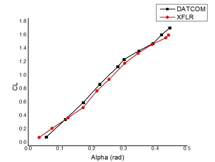
4. Comparison of Results
Results obtained from both pieces of software are presented in terms of dimensionless
aerodynamic coefficients for both longitudinal and lateral stability at low-cruise-flight
conditions. To validate the results expressed in terms of coefficients obtained from both
the commercial packages, these were compared with the analytical results available in the
literature [62]. The comparison of results shows that results obtained from computational
techniques are quite close to each other and the analytical results. However, a small
difference has been found in some of the coefficients. The comparison of results for
both longitudinal and lateral coefficients obtained from both pieces of software with the
results available in the literature is summarized in Tables A1 and A2 of Appendix A. The
comparison of results shows that longitudinal coefficients obtained from DATCOM are
quite close to the analytical results; however, there is some difference in longitudinal and
lateral values. On the other hand, the XFLR results are very close to the analytical results
in both the cases. An old version of US DATCOM is available, and it was used during
the project. It has limitations for some input parameters and Mach number in some of the
analysis.
5. Analysis and Discussion
This paper reports the procedure for estimating the aerodynamic coefficients of a wide-
body aircraft (Boeing 747-200) using computational techniques. The major achievementYou can also read