Fisher Vector Faces in the Wild
←
→
Page content transcription
If your browser does not render page correctly, please read the page content below
SIMONYAN et al.: FISHER VECTOR FACES IN THE WILD                                                     1

Fisher Vector Faces in the Wild
Karen Simonyan                                              Visual Geometry Group
karen@robots.ox.ac.uk                                       Department of Engineering Science
Omkar M. Parkhi                                             University of Oxford
omkar@robots.ox.ac.uk
Andrea Vedaldi
vedaldi@robots.ox.ac.uk
Andrew Zisserman
az@robots.ox.ac.uk

                                                     Abstract
           Several recent papers on automatic face verification have significantly raised the per-
       formance bar by developing novel, specialised representations that outperform standard
       features such as SIFT for this problem.
           This paper makes two contributions: first, and somewhat surprisingly, we show that
       Fisher vectors on densely sampled SIFT features, i.e. an off-the-shelf object recognition
       representation, are capable of achieving state-of-the-art face verification performance on
       the challenging “Labeled Faces in the Wild” benchmark; second, since Fisher vectors
       are very high dimensional, we show that a compact descriptor can be learnt from them
       using discriminative metric learning. This compact descriptor has a better recognition
       accuracy and is very well suited to large scale identification tasks.

1     Introduction
Face identification, i.e. the problem of inferring the identity of people from pictures of their
face, is a key area of research in image understanding. Beyond its scientific interest, this
problem has numerous and important applications in surveillance, access control, and search.
Automatic Face Verification (AFV) is a formulation of the face identification problem where
the task is to determine whether two images depict the same person or not. In the past few
years, the dataset “Labeled Faces in the Wild” (LFW) [13] has become the de-facto eval-
uation benchmark for AFV, promoting the rapid development of new and significantly im-
proved AFV methods. Recent efforts, in particular, have focused on developing new image
representations and combination of features specific to AFV to surpass standard representa-
tions such as SIFT [21]. The question that this paper addresses is what happens if, instead
of developing yet another face-specific image representation, one applies off-the-shelf object
recognition representations to AFV.
    The results are striking. Our first contribution is to show that dense descriptor sampling
combined with the improved Fisher Vector (FV) encoding of [24] (Sect. 2) outperforms or
performs just as well as the best face verification representations, including the ones that use
elaborate face landmark detectors [3, 6] and multiple features [12]. The significance of this
 c 2013. The copyright of this document resides with its authors.
It may be distributed unchanged freely in print or electronic forms.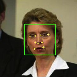
2                                    SIMONYAN et al.: FISHER VECTOR FACES IN THE WILD

result is that FVs are not specific to faces, having been proposed for object recognition in
general. However, FV descriptors are high-dimensional, which may be impractical in com-
bination with huge face databases. Our second contribution is to show that FV face repre-
sentations are amenable to discriminative dimensionality reduction using a linear projection,
which leads simultaneously to a significant dimensionality reduction as well as improved
recognition accuracy (Sect. 3). The processing pipeline (Sect. 4) is illustrated in Fig. 1. Our
end result is a compact discriminative descriptor for face images that achieves state-of-the-
art performance on the challenging LFW dataset in both restricted and unrestricted settings
(Sect. 5).

1.1    Related work
Face identification approaches. Face recognition research has been focusing on five ar-
eas: face detection, facial landmark detection, face registration, face description, and sta-
tistical learning. A typical face recognition system requires all these steps, but many works
focus on a few of these aspects in order to improve the overall system performance. For facial
landmark detection, Everingham et al. [9] proposed pictorial structures, Dantone et al. [8]
conditional random forests, and Zhu et al. [43] deformable parts models. Several papers
investigated face descriptors, including LBP and its variants [5, 6, 12, 20, 22, 25, 33, 38, 39],
SIFT [10, 20], and learnt representations [25, 40]. In [29], the Fisher vector encoding of local
intensity differences was used as a face descriptor. Another interesting approach is to learn
and extract semantic face attributes as facial features for identification and other tasks [3, 17].
Statistical learning is generally used to map face representations to a final recognition re-
sult, with metric or similarity learning being the most popular approach, particularly for
AFV [6, 10, 12, 22, 41]. Another popular approach is based on exemplar SVMs [33, 38, 39].

Dense features and their encodings for generic object recognition. Dense feature ex-
traction is an essential component of many state-of-the-art image classification methods [18,
23, 27]. The idea is to compute features such as SIFT densely on an image, rather than
on a sparse and potentially unreliable set of points obtained from an interest point detector.
Dense features are then encoded into a single feature vector, summarising the image con-
tent in a form suitable for learning and recognition. The best known encoding is probably
the Bag-of-Visual-Words (BoVW) model [7, 31], which builds a histogram of occurrences
of vector-quantised descriptors. More recent encodings include VLAD [15], Fisher Vectors
(FVs) [24], and Super Vector Coding [42]. A common aim of these encodings is to reduce the
loss of information introduced by the vector quantisation step in BoVW. In [4] it was shown
that FVs outperform the other encodings on a number of image recognition benchmarks, so
we adopt them here for face description.

Discriminative dimensionality reduction. The aim of discriminative dimensionality re-
duction is to obtain smaller image descriptors, while preserving or even improving their
ability to discriminate images based on their content. This is often formalised as the prob-
lem of finding a low-rank linear projection W of the descriptors that minimises the dis-
tances between images with the same content (e.g. same face) and maximises it otherwise.
“Fisherfaces” [2] is one of the early examples of discriminative learning for dimensionality
reduction, applied to face recognition. A closely related formulation is that of learning a Ma-
halanobis matrix M = W >W , a problem that has convex formulations [37], even in the case
SIMONYAN et al.: FISHER VECTOR FACES IN THE WILD                                                3

    Facial landmark    Aligned and         Dense SIFT,         Discriminative      Compact face
       detection       cropped face        GMM, and FV         dim. reduction      representation

Figure 1: Method overview: a face is encoded in a discriminative compact representa-
tion

of low-rank constraints [30]. However, learning the matrix M is practical only if the starting
dimensionality of the descriptor is moderate (e.g. less than 1000 dimensions), so different
approaches are required otherwise. One approach is to first reduce the dimensionality gen-
eratively, for example by using PCA, and then perform metric learning in a low-dimensional
space [6, 10], but this is suboptimal as the first step may lose important discriminative infor-
mation. Another approach, which we use here, is to optimise directly the projection matrix
W , as its size depends on the reduced dimensionality, although this results in a non-convex
formulation [11, 34].

2      Fisher vector faces representation
Dense features. The FV construction starts by extracting patch features such as SIFT [21]
from the image. Rather than sampling locations and scales sparsely by running a carefully
tuned face landmark detector, our approach extracts features densely in scale and space.
Specifically, 24 × 24 pixels patches are sampled with a stride of one pixel and for each
patch the root-SIFT representation of [1] (referred simply as “SIFT” in√the following) is
computed. The process is repeated at five scales, with a scaling factors of 2. The procedure
is run (unless otherwise noted) after cropping and rescaling the face to a 160 × 125 image,
resulting in about 26K 128-dimensional descriptors per face. To aggregate these descriptors,
the non-linear FV encoding is used, as described briefly below.

Fisher vectors. The FV encoding aggregates a large set of vectors (e.g. the dense SIFT
features just extracted) into a high-dimensional vector representation. In general, this is
done by fitting a parametric generative model, e.g. the Gaussian Mixture Model (GMM), to
the features, and then encoding the derivatives of the log-likelihood of the model with respect
to its parameters [14]. Following [24], we train a GMM with diagonal covariances, and only
consider the derivatives with respect to the Gaussian mean and variances. This leads to the
representation which captures the average first and second order differences between the
(dense) features and each of the GMM centres:
                   N                                           N
                                                                          (x p − µk )2

     (1)      1               x p − µk        (2)       1
  Φk = √ ∑ α p (k)                       , Φk = √             ∑ p α (k)                − 1  (1)
           N wk p=1               σk                 N 2wk p=1                 σk2

Here, {wk , µk , σk }k are the mixture weights, means, and diagonal covariances of the GMM,
which is computed on the training set and used for the description of all face images; α p (k) is
the soft assignment weight of the p-th feature x p to the k-th Gaussian. An FV φ is obtained
4 SIMONYAN et al.: FISHER VECTOR FACES IN THE WILD
h i
(1) (2) (1) (2)
by stacking the differences: φ = Φ1 , Φ1 , . . . , ΦK , ΦK . The encoding describes how
the distribution of features of a particular image differs from the distribution fitted to the
features of all training images.
To make the dense patch features amenable to the FV description based on the diagonal-
covariance GMM, they are first decorrelated by PCA. In our experiments, we applied PCA to
SIFT, reducing its dimensionality from 128 to 64. The FV dimensionality is 2Kd, where K is
the number of Gaussians in the GMM, and d is the dimensionality of the patch feature vector.
We note that even though FV dimensionality is high (65536 for K = 512 and d = 64), it is
still significantly lower than the dimensionality of the vector obtained by stacking all dense
features (1.7M in our case). Following [24], the performance of an FV is further improved
by passing it through signed square-rooting and L2 normalisation.
Spatial information. The Fisher vector is an effective encoding of the feature space struc-
ture. However, it does not capture the distribution of features in the spatial domain. Several
ways of incorporating the spatial information have been proposed in the literature. In [24],
a spatial pyramid coding [18] was used, which consists in dividing an image into a num-
ber of cells and then stacking the FVs computed for each of these cells. The disadvantage
of such approach is that the dimensionality of the final image descriptor increases linearly
with the number of cells. In [16], a generative model (e.g. GMM) was learnt for the spatial
location of each visual word, and FV was used to encode both feature appearance and loca-
tion. Here we employ a related approach of [28], which consists in augmenting the visual
features with their spatial coordinates, and then using the FV encoding of the augmented
features as the image descriptor. In more detail, our dense features have the following form:
Sxy ; wx − 12 ; hy − 21 , where Sxy is the (PCA-SIFT) descriptor of a patch centred at (x, y), and
w and h are the width and height of the face image. The resulting FV dimensionality is thus
67584. Fig. 2 illustrates how Gaussian mixture components are spatially distributed over a
face when learnt for a face verification task.
3 Large-margin dimensionality reduction
In this section we explain how a high-dimensional FV encoding (Sect. 2) is compressed to
a small discriminative representation. The compression is carried out using a linear projec-
tion, which serves two purposes: (i) it dramatically reduces the dimensionality of the face
descriptors, making them applicable to large-scale datasets; and (ii) it improves the recogni-
tion performance by projection onto a subspace with a discriminative Euclidean distance.
In more detail, the aim is to learn a linear projection W ∈ R p×d , p
d, which projects
high-dimensional Fisher vectors φ ∈ Rd to low-dimensional vectors W φ ∈ R p , such that the
squared Euclidean distance dW 2 (φ , φ ) = kW φ − W φ k2 between images i and j is smaller
i j i j 2
than a learnt threshold b ∈ R if i and j are the same person, and larger otherwise. We
further impose that these conditions are satisfied with a margin of at least one, resulting in
the constraints:
2
yi j b − dW (φi , φ j ) > 1 (2)
where yi j = 1 iff images i and j contain the faces of the same person, and yi j = −1 otherwise.
Note that the Euclidean distance in the p-dimensional projected space can be seen as a
low-rank Mahalanobis metric in the original d-dimensional space:
2
dW (φi , φ j ) = kW φi −W φ j k22 = (φi − φ j )T W T W (φi − φ j ), (3)SIMONYAN et al.: FISHER VECTOR FACES IN THE WILD 5
where W T W ∈ Rd×d is the Mahalanobis matrix defining the metric. Due to the factorisation,
the Mahalanobis matrix W T W has rank equal to p, i.e. much smaller than the full rank d. As
a consequence, learning the projection matrix W is the same as learning a low-rank metric
W T W . Direct optimisation of the Mahalanobis matrix is however quite difficult, as the latter
has over 2 billion parameters for the d = 67K dimensional FVs. On the contrary, W has
pd = 8.5M parameters for p = 128, which can be learnt in the large scale learning scenario.
Learning W optimises the following objective function, incorporating the constraints (2)
in a hinge-loss formulation:
arg min ∑ max 1 − yi j b − (φi − φ j )T W T W (φi − φ j ) , 0
(4)
W,b i, j
The minimiser of (4) is found using a stochastic sub-gradient method. At each iteration t, the
algorithm samples a single pair of face images (i, j) (sampling with equal frequency positive
and negative labels yi j ) and performs the following update of the projection matrix:
(
2 (φ , φ ) > 1
Wt if yi j b − dW i j
Wt+1 = (5)
Wt − γyi jWt ψi j otherwise
where ψi j = (φi − φ j )(φi − φ j )T is the outer product of the difference vectors, and γ is a
constant learning rate, determined on the validation set. Note that the projection matrix Wt
is left unchanged if the constraint (2) is not violated, which speed-ups learning (due to the
large size of W , performing matrix operations at each iteration is costly). We choose not to
regularise W explicitly; rather, the algorithm stops after a fixed number of learning iterations
(1M in our case).
Finally, note that the objective (4) is not convex in W , so initialisation is important. In
practice, we initialise W to extract the p largest PCA dimensions. Furthermore, differently
from standard PCA, we equalise the magnitude of the dominant eigenvalues (whitening)
as the less frequent modes of variation tend to be amongst the most discriminative. It is
important to note that PCA-whitening is only used to initialise the learning process, and the
learnt metric substantially improves over its initialisation (Sect. 5). In particular, this is not
the same as learning a metric on the low-dimensional PCA-whitened data (p2 parameters);
instead, a projection W on the original descriptors is learnt (pd
p2 parameters), which
allows us to fully exploit the available supervision.
4 Implementation details and extensions
Face alignment and extraction. Given an image, we first run the Viola Jones detector [36]
to obtain the face detection. Using this detection, we then detect nine facial landmark po-
sitions using the publicly available code of [9]. Similar to them, we then apply similarity
transformation using all these points to transform a face to a canonical frame. In the aligned
image, we extract a 160 × 125 face region around the landmarks for further processing.
Face descriptor computation. For dense SIFT computation and Fisher vector encoding,
we utilised publicly available packages [4, 35]. Dimensionality reduction learning is im-
plemented in MATLAB and takes a few hours to compute on a single core (for each split).
Given an aligned and cropped face image, our mexified MATLAB implementation takes 0.6s
to compute a descriptor on a single CPU core (in the case of 2 pixel SIFT density).6 SIMONYAN et al.: FISHER VECTOR FACES IN THE WILD
Diagonal “metric” learning. Apart from the low-rank Mahalanobis metric learning (Sect. 3),
we also consider diagonal metric learning on the full-dimensional Fisher vectors. It is carried
out using a conventional linear SVM formulation, where features are the vectors of squared
differences between the corresponding components of the two compared FVs. We did not
observe any improvement by enforcing the positivity of the learnt weights, so it was omitted
in practice (i.e. the learnt function is not strictly a metric).
Joint metric-similarity learning. Recently, a “joint Bayesian” approach to face similarity
learning has been employed in [5, 6]. It effectively corresponds to joint learning of a low-
rank Mahalanobis distance (φi − φ j )T W T W (φi − φ j ) and a low-rank kernel (inner product)
φiT V T V φ j between face descriptors φi , φ j . Then, the difference between the distance and
the inner product can be used as a score function for face verification. We consider it as
another option for comparing face descriptors (apart from the low-rank metric learning and
diagonal metric learning), and incorporate joint metric-similarity learning into our large-
margin learning formulation (4). In that case, we perform stochastic updates (5) on both
low-dimensional projections W and V .
Horizontal flipping. Following [12], we considered the augmentation of the test set by
taking the horizontal reflections of the two compared images, and averaging the distances
between the four possible combinations of the original and reflected images.
5 Experiments
5.1 Dataset and evaluation protocol
Our framework is evaluated on the popular “Labeled Faces in the Wild dataset” (LFW) [13].
The dataset contains 13233 images of 5749 people downloaded from the Web and is con-
sidered the de-facto standard benchmark for automatic face verification. For evaluation, the
data is divided into 10 disjoint splits, which contain different identities and come with a
list of 600 pre-defined image pairs for evaluation (as well as training as explained below).
Of these, 300 are “positive” pairs portraying the same person and the remaining 300 are
“negative” pairs portraying different people.
We follow the recommended evaluation procedure [13] and measure the performance of
our method by performing a 10 fold cross validation, training the model on 9 splits, and
testing it on the remaining split. All aspects of our method that involve learning, including
PCA projections for SIFT, Gaussian mixture models, and the discriminative Fisher vector
projections, were trained independently for each fold.
Two evaluation measures are considered. The first one is the Receiving Operating Char-
acteristic Equal Error Rate (ROC-EER), which is the accuracy at the ROC operating point
where the false positive and false negative rates are equal [10]. This measure reflects the
quality of the ranking obtained by scoring image pairs and, as such, is independent on the
bias learnt in (2). ROC-EER is used to compare the different stages of the proposed frame-
work. In order to allow a direct comparison with published results, however, our final clas-
sification performance is also reported in terms of the classification accuracy (percentage of
image pairs correctly classified) – in this case the bias is important.
LFW specifies a number of evaluation protocols, two of which are considered here. In
the “restricted setting”, only the pre-defined image pairs for each of the splits (fixed by theSIMONYAN et al.: FISHER VECTOR FACES IN THE WILD 7
LFW creators) can be used for training. Instead, in the “unrestricted setting” one is given
the identities of the people within each split and is allowed to form an arbitrary number, in
practice much larger, of positive and negative pairs for training.
5.2 Framework parameters
First, we explore how the different parameters of the method affect its performance. The
experiments were carried out in the unrestricted setting using unaligned LFW images and a
simple alignment procedure described in Sect. 4. We explore the following settings: SIFT
density (the step between the centres of two consecutive descriptors), the number of Gaus-
sians in the GMM, the effect of spatial augmentation, dimensionality reduction, distance
function, and horizontal flipping. The results of the comparison are given in Table 1. As can
be seen, the performance increases with denser sampling and more clusters in the GMM.
Spatial augmentation boosts the performance with only a moderate increase in dimensional-
ity (caused by the addition of the (x, y) coordinates to 64-D PCA-SIFT). Our dimensionality
reduction to 128-D achieves 528-fold compression and further improves the performance.
We found that using projection to higher-dimensional spaces (e.g. 256-D) does not improve
the performance, which can be caused by overfitting.
As far as the choice of the FV distance function is concerned, a low-rank Mahalanobis
metric outperforms both full-rank diagonal metric and unsupervised PCA-whitening, but is
somewhat worse than the function obtained by the joint large-margin learning of the Ma-
halanobis metric and inner product. It should be noted that the latter comes at the cost of
slower learning and the necessity to keep two projection matrices instead of one. Finally,
using horizontal flipping consistently improves the performance. In terms or the ROC-EER
measure, our best result is 93.13%.
SIFT GMM Spatial Desc. Distance Hor. ROC-
density Size Aug. Dim. Function Flip. EER,%
2 pix 256 32768 diag. metric 89.0
2 pix 256 X 33792 diag. metric 89.8
2 pix 512 X 67584 diag. metric 90.6
1 pix 512 X 67584 diag. metric 90.9
1 pix 512 X 128 low-rank PCA-whitening 78.6
1 pix 512 X 128 low-rank Mah. metric 91.4
1 pix 512 X 256 low-rank Mah. metric 91.0
1 pix 512 X 128 low-rank Mah. metric X 92.0
1 pix 512 X 2×128 low-rank joint metric-sim. 92.2
1 pix 512 X 2×128 low-rank joint metric-sim. X 93.1
Table 1: Framework parameters: The effect of different FV computation parameters and
distance functions on ROC-EER. All experiments done in the unrestricted setting.
5.3 Learnt projection model visualisation
Here we demonstrate that the learnt model can indeed capture face-specific features. To
visualise the projection matrix W , we make use of the fact that each GMM component corre-
sponds to a part of the Fisher vector and, in turn, to a group of columns in W . This makes it
possible to evaluate how important certain Gaussians are for comparing human face images8 SIMONYAN et al.: FISHER VECTOR FACES IN THE WILD
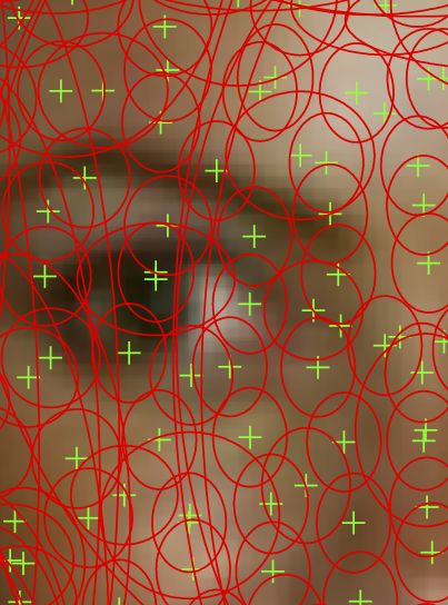
(a) (b) (c) (d) (e)
Figure 2: Coupled with discriminative dimensionality reduction, a Fisher vector can
automatically capture the discriminative parts of the face. (a): an aligned face image;
(b): unsupervised GMM clusters densely span the face; (c): a close-up of a face part covered
by the Gaussians; (d): 50 Gaussians corresponding to the learnt projection matrix columns
with the highest energy; (e): 50 Gaussians corresponding to the learnt projection matrix
columns with the lowest energy.
by computing the energy (Euclidean norm) of the corresponding column group. In Fig. 2
we show the GMM components which correspond to the groups of columns with the highest
and lowest energy. Each Gaussian captures joint appearance-location statistics (Sect. 2), but
here we only visualise the location as an ellipse with the centre and radii set to the mean and
variances of the spatial components. As can be seen from Fig. 2-d, the 50 Gaussians cor-
responding to the columns with the highest energy match the facial features without being
explicitly trained to do so. They have small spatial variances and are finely localised on the
image plane. On the contrary, Fig. 2-e shows how the 50 Gaussians corresponding to the
columns with the lowest energy cover the background areas. These clusters are deemed as
the least meaningful by our projection learning; note that their spatial variances are large.
5.4 Comparison with the state of the art
Unrestricted setting. In this scenario, we compare against the best published results ob-
tained using both single (Table 2, left-bottom) and multi-descriptor representations (Table 2,
left-top). Similarly to the previous section, the experiments were carried out using unaligned
LFW images, processed as described in Sect. 4. This means that the outside training data is
only utilised in the form of a simple landmark detector, trained by [9].
Our method achieves 93.03% face verification accuracy, closely matching the state-of-
the-art method of [6], which achieves 93.18% using LBP features sampled around 27 land-
marks. It should be noted that (i) the best result of [6] using SIFT descriptors is 91.77%;
(ii) we do not rely on multiple landmark detection, but sample the features densely. The
ROC curves of our method as well as the other methods are shown in Fig. 3.
Restricted setting. In this strict setting, no outside training data is used, even for the land-
mark detection. Following [19], we used centred 150 × 150 crops of “LFW-funneled” im-
ages, provided as a part of the LFW dataset. We found that the limited amount of training
data, available in this setting, is insufficient for dimensionality reduction learning. Therefore,
we learnt a diagonal “metric” function using an SVM as described in Sect. 4. Achieving the
verification accuracy of 87.47%, our descriptor sets a new state of the art in the restricted set-
ting (Table 2, right), outperforming the recently published result of [19] by 3.4%. It shouldSIMONYAN et al.: FISHER VECTOR FACES IN THE WILD 9
ROC Curves − Unrestricted Setting ROC Curves − Restricted Setting
1 1
0.95 0.95
0.9 0.9
0.85 0.85
true positive rate
true positive rate
0.8 0.8
0.75 0.75
0.7 0.7
Our Method
0.65 high−dim LBP 0.65
CMD+SLBP
0.6 Face.com 0.6
CMD Our Method
0.55 LBP−PLDA 0.55 APEM−Fusion
LDML−MKNN V1−like(MKL)
0.5 0.5
0 0.2 0.4 0.6 0 0.2 0.4 0.6
false positive rate false positive rate
Figure 3: Comparison with the state of the art: ROC curves of our method and the state-
of-the-art techniques in LFW-unrestricted (left) and LFW-restricted (right) settings.
be noted that while [19] also use GMMs for dense feature clustering, they do not utilise the
compressed Fisher vector encoding, but keep all extracted features for matching, which im-
poses a limitation on the number of features that can be extracted and stored. In our case,
we are free from this limitation, since the dimensionality of an FV does not depend on the
number of features it encodes. The best result of [19] was obtained using two types of fea-
tures and GMM adaptation (“APEM Fusion”). When using non-adapted GMMs (as we do)
and SIFT descriptors (“PEM SIFT”), their result is 6% worse than ours.
Our results in both unrestricted and restricted settings confirm that the proposed face
descriptor can be used in both small-scale and large-scale learning scenarios, and is robust
with respect to the face alignment and cropping technique.
6 Conclusion
In this paper, we have shown that an off-the-shelf image representation based on dense SIFT
features and Fisher vector encoding achieves state-of-the-art performance on the challenging
“Labeled Faces in the Wild” dataset. The use of dense features allowed us to avoid applying
a large number of sophisticated face landmark detectors. Also, we have presented a large-
margin dimensionality reduction framework, well suited for high-dimensional Fisher vector
representations. As a result, we obtain an effective and efficient face descriptor computation
pipeline, which can be readily applied to large-scale face image repositories.
It should be noted that the proposed system is based upon a single feature type. In our
future work, we are planning to investigate multi-feature image representations, which can
be readily incorporated into our framework.
Acknowledgements
This work was supported by ERC grant VisRec no. 228180 and EU Project AXES ICT-
269980.10 SIMONYAN et al.: FISHER VECTOR FACES IN THE WILD
Unrestricted setting Restricted setting
Method Mean Acc. Method Mean Acc.
LDML-MkNN [10] 0.8750 ± 0.0040 V1-like/MKL [26] 0.7935 ± 0.0055
Combined multishot [33] 0.8950 ± 0.0051 PEM SIFT [19] 0.8138 ± 0.0098
Combined PLDA [20] 0.9007 ± 0.0051 APEM Fusion [19] 0.8408 ± 0.0120
face.com [32] 0.9130 ± 0.0030 Our Method 0.8747 ± 0.0149
CMD + SLBP [12] 0.9258 ± 0.0136
LBP multishot [33] 0.8517 ± 0.0061
LBP PLDA [20] 0.8733 ± 0.0055
SLBP [12] 0.9000 ± 0.0133
CMD [12] 0.9170 ± 0.0110
High-dim SIFT [6] 0.9177 ± N/A
High-dim LBP [6] 0.9318 ± 0.0107
Our Method 0.9303 ± 0.0105
Table 2: Left: Face verification accuracy in the unrestricted setting. Using a single
type of local features (dense SIFT), our method outperforms a number of methods, based on
multiple feature types, and closely matches the state-of-the-art results of [6]. Right: Face
verification accuracy in the restricted setting (no outside training data). Our method
achieves the new state of the art in this strict setting.
References
[1] R. Arandjelović and A. Zisserman. Three things everyone should know to improve
object retrieval. In Proc. CVPR, 2012.
[2] P. Belhumeur, J. Hespanha, and D. Kriegman. Eigenfaces vs. Fisherfaces: Recognition
using class specific linear projection. IEEE PAMI, 19(7):711–720, 1997.
[3] T. Berg and P. N. Belhumeur. Tom-vs-Pete classifiers and identity-preserving align-
ment for face verification. In Proc. BMVC., 2012.
[4] K. Chatfield, V. Lempitsky, A. Vedaldi, and A. Zisserman. The devil is in the details:
an evaluation of recent feature encoding methods. In Proc. BMVC., 2011.
[5] D. Chen, X. Cao, L. Wang, F. Wen, and J. Sun. Bayesian face revisited: A joint
formulation. In Proc. ECCV, pages 566–579, 2012.
[6] D. Chen, X. Cao, F. Wen, and J. Sun. Blessing of dimensionality: High dimensional
feature and its efficient compression for face verification. In Proc. CVPR, 2013.
[7] G. Csurka, C. Bray, C. Dance, and L. Fan. Visual categorization with bags of keypoints.
In Workshop on Statistical Learning in Computer Vision, ECCV, pages 1–22, 2004.
[8] M. Dantone, J. Gall, G. Fanelli, and L. van Gool. Real-time facial feature detection
using conditional regression forests. In Proc. CVPR, 2012.
[9] M. Everingham, J. Sivic, and A. Zisserman. Taking the bite out of automatic naming
of characters in TV video. Image and Vision Computing, 27(5), 2009.SIMONYAN et al.: FISHER VECTOR FACES IN THE WILD 11
[10] M. Guillaumin, J. Verbeek, and C. Schmid. Is that you? metric learning approaches for
face identification. In Proc. ICCV, 2009.
[11] M. Guillaumin, J. Verbeek, and C. Schmid. Multiple instance metric learning from
automatically labeled bags of faces. In Proc. ECCV, pages 634–647, 2010.
[12] C. Huang, S. Zhu, and K. Yu. Large scale strongly supervised ensemble metric learning,
with applications to face verification and retrieval. (TR115), 2011.
[13] G. B. Huang, M. Ramesh, T. Berg, and E. Learned-Miller. Labeled faces in the wild:
A database for studying face recognition in unconstrained environments. Technical
Report 07-49, University of Massachusetts, Amherst, 2007.
[14] T. Jaakkola and D. Haussler. Exploiting generative models in discriminative classifiers.
In NIPS, pages 487–493, 1998.
[15] H. Jégou, M. Douze, C. Schmid, and P. Pérez. Aggregating local descriptors into a
compact image representation. In Proc. CVPR, 2010.
[16] J. Krapac, J. Verbeek, and F. Jurie. Modeling spatial layout with fisher vectors for
image categorization. In Proc. ICCV, pages 1487–1494, 2011.
[17] N. Kumar, A. C. Berg, P. Belhumeur, and S. K. Nayar. Attribute and simile classifiers
for face verification. In Proc. ICCV, 2009.
[18] S. Lazebnik, C. Schmid, and J Ponce. Beyond Bags of Features: Spatial Pyramid
Matching for Recognizing Natural Scene Categories. In Proc. CVPR, 2006.
[19] H. Li, G. Hua, J. Brandt, and J. Yang. Probabilistic elastic matching for pose variant
face verification. In Proc. CVPR, 2013.
[20] P. Li, Y. Fu, U. Mohammed, J. H. Elder, and S. J. D. Prince. Probabilistic models for
inference about identity. IEEE PAMI, 34(1):144–157, Nov 2012.
[21] D. Lowe. Distinctive image features from scale-invariant keypoints. IJCV, 60(2):91–
110, 2004.
[22] H. V. Nguyen and L. Bai. Cosine similarity metric learning for face verification. In
Proc. Asian Conf. on Computer Vision, 2010.
[23] E. Nowak, F. Jurie, and B. Triggs. Sampling strategies for bag-of-features image clas-
sification. In Proc. ECCV, 2006.
[24] F. Perronnin, J. Sánchez, and T. Mensink. Improving the Fisher kernel for large-scale
image classification. In Proc. ECCV, 2010.
[25] N. Pinto and D. Cox. Beyond simple features: A large-scale feature search approach
to unconstrained face recognition. In Proc. Int. Conf. Autom. Face and Gesture Recog.,
2011.
[26] N. Pinto, J. J. DiCarlo, and D. D. Cox. How far can you get with a modern face
recognition test set using only simple features? In Proc. CVPR, 2009.12 SIMONYAN et al.: FISHER VECTOR FACES IN THE WILD
[27] J. Sánchez and F. Perronnin. High-dimensional signature compression for large-scale
image classification. In Proc. CVPR, 2011.
[28] J. Sánchez, F. Perronnin, and T. Emídio de Campos. Modeling the spatial layout of im-
ages beyond spatial pyramids. Pattern Recognition Letters, 33(16):2216–2223, 2012.
[29] G. Sharma, S. Hussain, and F. Jurie. Local higher-order statistics (LHS) for texture
categorization and facial analysis. In Proc. ECCV, 2012.
[30] K. Simonyan, A. Vedaldi, and A. Zisserman. Descriptor learning using convex optimi-
sation. In Proc. ECCV, 2012.
[31] J. Sivic and A. Zisserman. Video Google: A text retrieval approach to object matching
in videos. In Proc. ICCV, volume 2, pages 1470–1477, 2003.
[32] Y. Taigman and L. Wolf. Leveraging billions of faces to overcome performance barriers
in unconstrained face recognition. 2011.
[33] Y. Taigman, L. Wolf, and T. Hassner. Multiple one-shots for utilizing class label infor-
mation. In Proc. BMVC., 2009.
[34] L. Torresani and K. Lee. Large margin component analysis. In NIPS, pages 1385–1392.
MIT Press, 2007.
[35] A. Vedaldi and B. Fulkerson. VLFeat - an open and portable library of computer vision
algorithms. In ACM Multimedia, 2010.
[36] P. Viola and M. Jones. Robust real-time object detection. In IJCV, volume 1, 2001.
[37] K.Q. Weinberger, J. Blitzer, and L. Saul. Distance metric learning for large margin
nearest neighbor classification. In NIPS, 2006.
[38] L. Wolf, T. Hassner, and Y. Taigman. Descriptor based methods in the wild. In Faces
in Real-Life Images Workshop in European Conference on Computer Vision, 2008.
[39] L. Wolf, T. Hassner, and Y. Taigman. Similarity scores based on background samples.
In Proc. Asian Conf. on Computer Vision, 2009.
[40] Q. Yin, X. Tang, and Sun J. Face recognition with learning-based descriptor. In Proc.
CVPR, 2011.
[41] Y. Ying and P. Li. Distance metric learning with eigenvalue optimization. J. Machine
Learning Research, 2012.
[42] X. Zhou, K. Yu, T. Zhang, and T. S. Huang. Image classification using super-vector
coding of local image descriptors. In Proc. ECCV, 2010.
[43] X. Zhu and D. Ramanan. Face detection, pose estimation and landmark localization in
the wild. In Proc. CVPR, 2012.You can also read