FOG COMPUTING APPLICATION OF CYBER-PHYSICAL MODELS OF IOT DEVICES WITH SYMBOLIC APPROXIMATION ALGORITHMS
←
→
Page content transcription
If your browser does not render page correctly, please read the page content below
Fog Computing Application of Cyber-Physical Models of IoT Devices with Symbolic Approximation Algorithms Deok-Kee Choi ( dkchoi@dankook.ac.kr ) Dankook University Research Article Keywords: Cyber-Physical Model, Smart Manufacturing, IoT, Fog computing, Machine Learning, Symbolic Approximation Algorithms, Streaming Data Analytics Posted Date: June 4th, 2021 DOI: https://doi.org/10.21203/rs.3.rs-385990/v1 License: This work is licensed under a Creative Commons Attribution 4.0 International License. Read Full License
Choi
 1
 2
 3
 4
 5
      RESEARCH
 6
 7
 8
 9   Fog Computing Application of Cyber-Physical
10
11
12
     Models of IoT Devices with Symbolic
13
14
     Approximation Algorithms
15   Deok-Kee Choi
16
17
18
19      Abstract
20
        Smart manufacturing systems transmit out streaming data from IoT devices to cloud computing; however, this
21
        could bring about several disadvantages such as high latency, immobility, and high bandwidth usage, etc. As
22
23      for streaming data generated in many IoT devices, to avoid a long path from the devices to cloud computing,
24      Fog computing has drawn in manufacturing recently much attention. This may allow IoT devices to utilize the
25      closer resource without heavily depending on cloud computing. In this research, we set up a three-blade fan as
26      IoT device used in manufacturing system with an accelerometer installed and analyzed the sensor data through
27      cyber-physical models based on machine learning and streaming data analytics at Fog computing. Most of the
28      previous studies on the similar subject are of pre-processed data open to public on the Internet, not with
29      real-world data. Thus, studies using real-world sensor data are rarely found. A symbolic approximation
30      algorithm is a combination of the dictionary-based algorithm of symbolic approximation algorithms and
31      term-frequency inverse document frequency algorithm to approximate the time-series signal of sensors. We
32      closely followed the Bayesian approach to clarify the whole procedure in a logical order. In order to monitor a
33      fan’s state in real time, we employed five different cyber-physical models, among which the symbolic
34      approximation algorithm resulted in about 98% accuracy at a 95% confidence level with correctly classifying
35      the current state of the fan. Furthermore, we have run statistical rigor tests on both experimental data and the
36      simulation results through executing the post-hoc analysis. By implementing micro-intelligence with a trained
37      cyber-physical model unto an individual IoT device through Fog computing we may alienate significant amount
38      of load on cloud computing; thus, with saving cost on managing cloud computing facility. We would expect
39
        that this framework to be utilized for various IoT devices of smart manufacturing systems.
40
41      Keywords: Cyber-Physical Model; Smart Manufacturing; IoT; Fog computing; Machine Learning; Symbolic
42      Approximation Algorithms; Streaming Data Analytics
43
44
45
46
     Introduction                                                             [9, 10]. Cloud computing with big data analytics de-
     Smart manufacturing with IoT brings about rapid                          mands much expensive computing resources; therefore,
47
     manufacturing by networking machines, sensors, and                       downsizing the process being sent to cloud computing
48
49   actuators as a whole [1–3]. The economics of Indus-                      may be quite beneficial.
50   trial IoT is expected to grow up to $6.2 trillion by                       What smart manufacturing concerns most is to ac-
51   2025 [4]. IoT structure can be divided into three lev-                   cess the state of installed devices in real-time. Imple-
52   els: IoT device (embedded computing), Fog comput-                        menting any complexity of intelligence that can rec-
53   ing, and Cloud computing. Each level is distinguished                    ognize the state of devices into embedded computing
54   by the use of the three different data analytics shown in                is often not possible due to its lack of built-in com-
55   Fig. 1. Fog computing is facility that uses edge devices
                                                                              puting resources. This calls for a cyber-physical model
56   to carry out fast streaming data analytics [5–8]. The
                                                                              (CPM) [11, 12] that can make an important decision
57   characteristics of Fog computing are a) low latency,
                                                                              on its own at Fog computing. However, no matter how
58   b) low data bandwidth, and c) sensor heterogeneity
                                                                              simple an IoT device operates in a certain way, it is
59   Correspondence: dkchoi@dankook.ac.kr                                     very difficult to create a CPM that can accurately tell
60   Department of Mechanical Engineering, Dankook University, 152,
     Jukjeon-ro, Suji-gu, 16890 Yongin-si, Gyeonggi-do, Republic of Korea     the state on its own subject to unknown external or
61
62   Full list of author information is available at the end of the article   internal elements.
63
64
65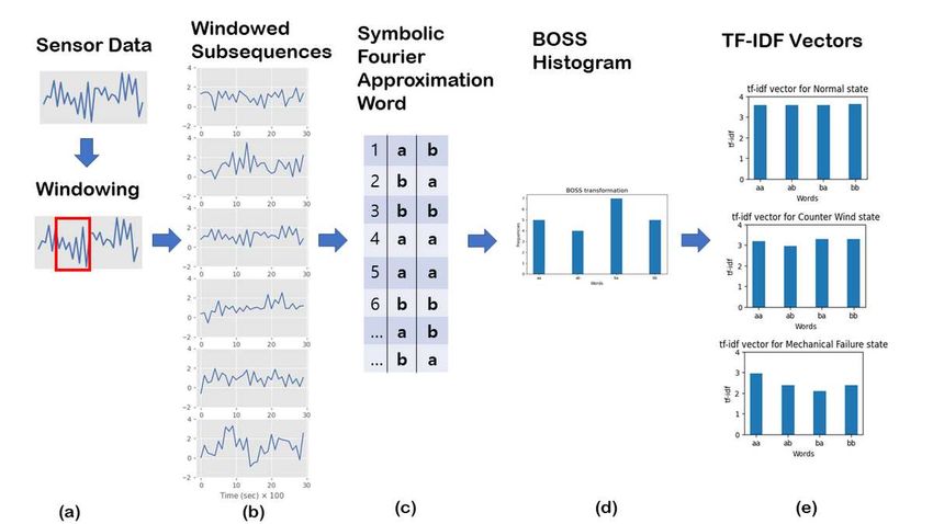
Choi                                                                                                      Page 2 of 11
 1
 2
 3
 4
 5
 6      Yet another difficult issue can be how to process         In this study, we built a three-blade fan with an ac-
 7   enormous streaming data from sensors with great ef-        celerometer installed on it. We defined three states of
 8   ficiency. This type of data is called time series (TS),    the fan for classification: normal state, counter-wind
 9   which is a collection of ordered values over time. Since   state, and mechanical failure state. Fog computing is
10   TS has a temporal structure, it needs to be treated        set up with a system: Intel Core i3-8100 CPU 3.60 GHz
11   differently from other types of data [13]. One big         at 4 GB memory, and the OS being Ubuntu 20.04.1
12   challenge in dealing with TS is its vast size [14]. In     LTS.
13   general, by applying approximation or transformation         In summary, herein we pursued three objectives:
14   to data, some amount of size and noise can be cut          along with real-world experimental data of the fan,
15   down. Being used as a baseline algorithm for TS, K-        we proposed a cyber-physical model that meets the
16   Nearest Neighbors (KNN) with Dynamic Time Warp-            following requirements:
17   ing (DTW) is quite slow and requires much computing           • To be able to efficiently process streaming data,
18   resources [15]. Recently, two Symbolic Approximation
                                                                   • To be able to accurately classify the state of the
19   Algorithms that serve to transform a TS into symbols
                                                                     fan,
20   have drawn good attention: One is Symbolic Aggre-
21                                                                 • To complete classification within the designated
     gate approXimation (SAX) [16]. The other is Symbolic
22                                                                   time at Fog computing.
     Fourier Approximation (SFA) [17], through which we
23   carried out simulations in this study. SFA consists of
24   Discrete Fourier Transform (DFT) for approximation         Cyber-Physical Models for IoT Device
25   and Multiple Coefficient Binning (MCB) for quantiza-       In probabilistic modeling, we pay good attention to
26   tion.                                                      a model for real-world phenomena with uncertainty.
27      Given TS, time series classification (TSC) is of de-    Unlike with well-organized and preprocessed data, the
28   termining to which of a set of designated classes in       complexity of the real-world phenomenon as shown in
29
     this TS belongs to, the classes being defined by mul-      Fig. 3 can easily go out of the bound of our com-
30
     tiple set of training data [18, 19]. As the heart of the   prehension. For example, such are air velocity, rota-
31
     intelligence of IoT, CPM is evolving in such a way         tion, vibration, counter-wind occurrence, and pressure
32
33   that it can manipulate the physical processes based on     changes, etc. This is because there are too many un-
34   the domain-specific knowledge on its own, not blindly      knowns relating physical interactions for even a simple
35   transmitting data to a cloud system for a request for      IoT device like a fan.
36   an important decision. Recently, a couple of interest-       We have sought a cyber-physical model that can
37   ing algorithms for TSC have been rolled out: the BOSS      classify the state (or class) of a fan. The class set
38   model [20] and the WEASEL MUSE model [21] both             C = {C1 , · · · , CK } with K being the number of the
39   apply a supervised symbolic representation to trans-       classes, which the classes are normal, counter-wind,
40   form subsequences to words for classification. Several     and mechanical failure states of the fan in this study.
41   machine learning techniques have been used such as lo-     Fast Streaming data from sensors can be regarded as
42   gistic regression, support vector machine, random for-
                                                                time series. A time series Ti is defined as an ordered
43   est, artificial neural networks (ANN) [22], and LSTM
                                                                sequence Ti = {t1 , . . . , tn }. The multivariate time se-
44   [23]. In this study, we employed the BOSS model as an
                                                                ries have several features, that is ∀j, tj ∈ Rd , where
45   algorithm for the CPM. Furthermore, we adopt an ex-
                                                                d is the number of features. The model is expected
46   tended algorithm: BOSS VS (Bag-Of-Symbolic Fourier
                                                                to provide a relatively simple function f : T → C,
47   Symbols in Vector Space) based on a term-frequency
48   inverse-term-frequency vector for each class [24, 25].     where T = {T1 , . . . , TN }, and is expressed as a joint
49      Figure 2 shows a workflow, on which we divided it       probability distribution p(C, T).
50   into three phases: observation, machine learning, and        A prime purpose of the use of the Bayesian approach
51   status update. In the observation phase, streaming         is to infer probability for what we are interested in. As
52   data is being stored for 3T sec. Once it passes 3T sec,    shown in Fig. 3, because the inference in such a phe-
53   then Machine Learning trains the model for 2T sec. It      nomenon is quite complex, the model demands a huge
54   should be noted that even while learning the model,        amount of training data. For such a practical reason,
55   the new data is still coming in to be stored. As soon      the number of cases within the model of the joint prob-
56   as the training is up, the model conducts classification   ability must be drastically reduced. That is, firstly we
57                                                              worked with the joint probability distribution p(C, T)
     over new data for T sec. It is important to note that
58                                                              of the class C and a time series T. We wanted to cal-
     Machine Learning and Status Update must be com-
59
     pleted within 3T sec, otherwise, this process can be       culate how likely a given data is. Thus, we defined the
60
     out of work. This completes a single process loop in       posterior p(C|T) to infer the hidden structure with
61
62   the repetitive process for classification.                 Bayesian inference:
63
64
65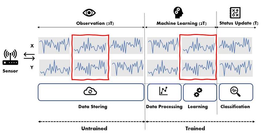
Choi Page 3 of 11
1
2
3
4
5
6 constructed using the Fourier transform of N training
7 time series with the first l of Fourier coefficients being
8 f (T) = argmax p(C|T) equivalent to an SFA word of length l as defined in
C∈C
9 Eq.(4).
10 p(T|C)p(C)
= argmax R (1)
11 C∈C p(T|C)p(C)dC DFT(T1 )
12 ∝ argmax p(T|C)p(C) M=
..
C∈C
.
13
DFT(TN )
14
By marginalizing the joint probability distribution
15 (a1 , b1 )1 ... (al/2 , bl/2 )1
16 over C we are not interested in, then we R can make the .. .. ..
= (4)
resulting marginal distribution p(T) = p(T|C)p(C)dC. . . .
17
18 This calls for the conditioning on the joint probability (a1 , b1 )N ... (al/2 , bl/2 )N
19 and prior: p(T|C)p(C). Once given the training data
20 set, the likelihood p(T|C) in Eq. (1) can be calculated. where Mj being j −th column of M matrix for all of N
21 Thereby, we can then answer: given the data T, what training data. Mi is then divided into intervals of c and
22 are the most likely parameters of the model or class C? is sorted by value and then divided into c bins of equi-
23 With the help of the Bayesian approach, we may come depth policy. That is, the i − th row of M corresponds
24 up with a logical procedure empolyed in the present to the Fourier transform of the ith time series Ti . With
25 study. the columns Mj for j = 1, . . . , l, and an alphabet space
26 Classification refers to labeling a new time series Al of size c, the breakpoints βj (0) < · · · < βj (c) for
27 Q = {q1 , · · · , qm } and ∀i, qi ∈ Rd for i = 1 . . . m with each column Mj are generated. Each bin is labeled by
28 d being the feature shown in Eq.(2). In other words, applying the ath symbol of the alphabet Al to it. For
29
classification indicates the calculation of p(C|Q) sub- all combination of (j, a) with j = 1, . . . , l and a =
30 1, . . . , c, the labeling symbol(a) for Mj can be done by
jected to new streaming data Q = {Q1 , . . . , QN }:
31
32
33 [βj (a − 1), βj (a)] ≈ symbol(a) (5)
34 label(Q) = argmax p(C|Q)
Ck ∈C
35 It is noted that this process in Eq.(5) applies to all
36 = argmax p(Q|C)p(C) (2)
Ck ∈C training data.
37
38
39
Symbolic Fourier Approximation (SFA) SFA Working Example
This section introduces Symbolic Fourier Approxima- SFA word can be obtained from SFA(T) = s1 , . . . , sl
40
tion (SFA) used in the BOSS VS model. SFA consists with DFT where DFT(T) = t′1 , . . . , t′l and t′ s are trans-
41
42 of Discrete Fourier Transformation (DFT), and Mul- formed time series with Fourier transform. That is,
43 tiple Coefficient Binning (MCB). SFA: Rl → Al , where Al is the alphabet set of which
44 size is c. For a working example, in Fig. 5, we set l = 1
45 Discrete Fourier Transformation (DFT) and c = 2. Six samples as shown Fig. 5(a) are ran-
46 Discrete Fourier Transform (DFT) extracts Fourier co- domly selected from the experimental data. The data
47 efficients from each time series T : then is transformed via DFT, resulting in the Fourier
48 coefficients for each sample. A vector of the Fourier co-
49 efficient values of the first sample reads (-1.352, 5.043)
50 DFT(T ) = {a1 , b1 , . . . , am , bm } (3) as shown in Fig. 5(b). Next, MCB is conducted with
51 an alphabet set A1 = {aa, ab, ba, bb} as shown in
52 where ai and bi are the real and the imaginary element Fig. 5(c). Thereby, an SFA word of the first sample
53 of Fourier coefficients. Figure 4 shows that low-pass is mapped into a word ab shown in Fig. 5(d). Like-
54 filtering and smoothing of a sample of acceleration in wise, the other samples can be transformed into their
55 x-axis upon Discrete Fourier Transform (DFT), where respective SFA words.
56 DFT result is obtained by taking first two Fourier co-
57 efficients in Eq.(3). BOSS: Bag-of-SFA-Symbols model
58
The Bag-Of-SFA-Symbols (BOSS) model is of the time
59
Multiple Coefficient Binning (MCB) series representation with the structure-based repre-
60
61 Next, the Multiple Coefficient Binning (MCB) quanti- sentation of the bag-of-words model. The sequence of
62 zation is carried out with training data. M matrix is SFA words for six samples in Fig. 5(d) reads as follows:
63
64
65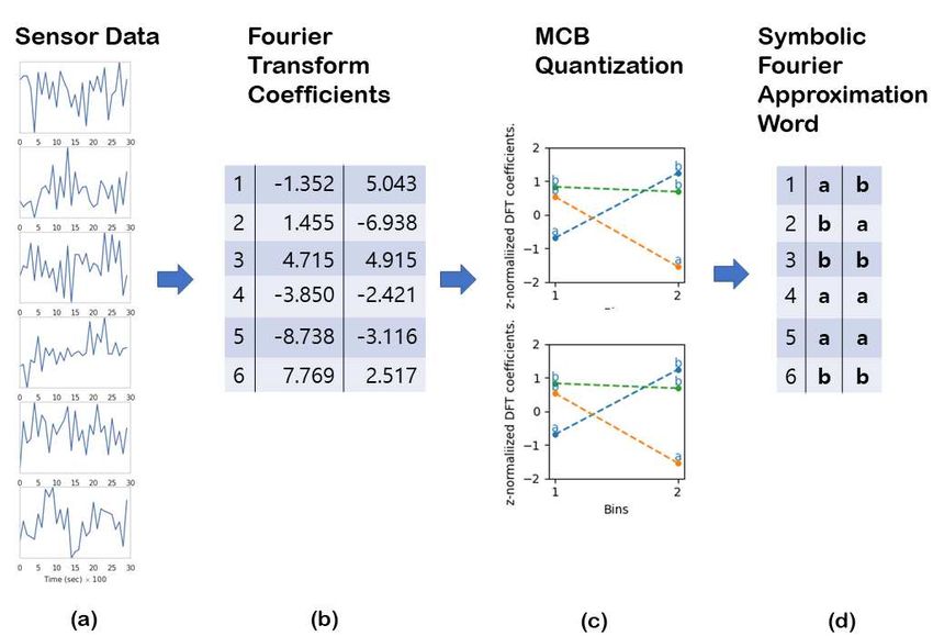
Choi                                                                                                            Page 4 of 11
 1
 2
 3
 4
 5
 6                                                                     where B(S) is the BOSS histogram in Eq.(7). The in-
 7                                                                     verse document frequency idf is given by
            S = {ab, ba, bb, aa, aa, bb}                        (6)
 8
                                                                                                        |C|
 9                                                                         idf(S, C) = log                                   (9)
     The values that count the apperance of SFA words in                                       |{C|T ∈ C ∩ B(S) > 0}|
10
     Eq.(6) are expressed upon numerosity reduction:
11
12                                                                       In this study, for classification purposes, we em-
13                                                                     ployed three different states of a running fan, which
            B : aa = 2, ab = 1, ba = 1, bb = 2                  (7)    is presented as a set of classes (states) C. The ele-
14
15                                                                     ments of the set are C = {C1 , C2 , C3 }. It is noted
     It is noted that SFA words in Eq.(6) now results in               that each element Ck for k = 1, 2, 3 represents a cer-
16
     the BOSS hisgogram shown in Eq.(7). Therefore, the                tain state of the fan. As for the human-readable for-
17
     BOSS model B can be regarded as a random variable,                mat, we have assigned name-tags to each class such
18
     that is, B : S → N . The probability mass function                as C1 = “N ormal”, C2 = “Counter W ind”, and
19
     p(B) can be addressed by p(B = aa) = 1/3, p(B =                   C3 = “M echanical F ailure”, respectively. The in-
20
21   ab) = 1/6, p(B = ba) = 1/6, and p(B = bb) =                       verse document frequency indicates the frequency of
22   1/3. This provides us with quite important information            an SFA word in a class Ck . Therefore, in this study,
23   about the structure of the samples, which structure is            the numerator of Eq.(9) of |C| denotes a numeric value
24   being used as features for machine learning.                      3. Multiplying Eq.(8) by Eq.(9), the tfidf of an SFA
25
     BOSS VS: Bag-of-SFA-Symbols in Vector Space                       word S within class C is defined as
26
     BOSS VS model is an extented BOSS model. A time
27
28   series T = {t1 , . . . , tn } of length n is divided into slid-       tfidf(S, C) = tf(S, C) · idf(S, C)
29   ing windows of length of w is Si,w , where w ∈ N .                                  "                   !#
30   The SFA word is defined as SFA(Si,w ) ∈ Al , with                                              X
                                                                                       = 1 + log        B(S)    ·
31   i = 1, 2, . . . , (n−w+1), where A is the SFA word space                                                               (10)
                                                                                                       T ∈C
32   and l ∈ N is the SFA word length. The BOSS his-
     togram B(S) : Al → N . The number in the histogram                                                 |C|
33                                                                                       log
     is the count of appearance of an SFA word within T                                        |{C|T ∈ C ∩ B(S) > 0}|
34
35   upon numerosity reduction. BOSS VS model allows
     frequent updates, such as fast streaming data analyt-             The result of tfidf(S, C) on three states is displayed
36
     ics. As shown in Fig. 6(a) and Fig. 6(b), the BOSS VS             in Fig. 6(e). It is noted that a high weight in Eq.(10) is
37
     model operates sliding windows unto each time series              obtained by a high term frequency in the given class.
38
39   resulting in multiple windowed subsequences. Next,
     each subsequence is tranformed into the SFA words                 Classification
40
41   shown in Fig. 6(c). All of the subsequences eventu-               Classification of new data Q can be carried out using
42   ally then result in the BOSS histogram shown in Fig.              the cosine similarity metric CosSim:
43   6(d). However, since the BOSS histogram itself is not
                                                                           CosSim(Q, C)
44   suitable for performing multiple of matrix calculations,                      P
45   it is vectorized through Term Frequency Inverse Doc-                              S∈Q tf(S, Q) · tfidf(S, C)      (11)
                                                                           = qP
46   ument Frequency (TF-IDF) algorithm shown in Fig.
                                                                                                 qP
                                                                                         2                      2
47   6(e).                                                                         S∈Q tf (S, Q)      S∈C tfidf (S, C)
48
49   TF-IDF: Term Frequency Inverse Document                           It is noted that in Eq.(11) tf(S, Q) is of the term
50   Frequency                                                         frequency of Q as shown in Fig.7(b), which is the
51   The BOSS VS model employs Term Frequency Inverse                  BOSS histogram of Q. Then, CosSim(Q, C) is calcu-
52   Document Frequency (TF-IDF) algorithm to weight                   lated in Eq.(11). Upon maximizing the cosine similar-
53   each term frequency in the vector. This assigns a                 ity, a query Q is thus classified into the class Ck as
54   higher weight to signify words of a class. The term fre-          shown in Eq.(12):
55   quency tf for SFA words S of a time series T within
56   class C is defined as
57                                                                         label(Q) = arg max (CosSim(Q, Ck ))              (12)
58                                                                                             Ck ∈C

59   tf(S, C)
                                                                         In conclusion, BOSS VS algorithm of which founda-
60      (         P                       P
                                                          (8)
          1 + log   T ∈C B(S) ,         if   T∈C B(S) > 0              tion is composed of two notions: Bag-of-words and TF-
61    =
62        0,                            otherwise                      IDF. What makes BOSS VS be different from other
63
64
65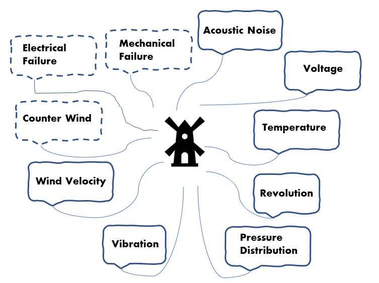
Choi Page 5 of 11
1
2
3
4
5
6 algorithms is a way of taking features of data. This In addition, we need to know how much trends, rep-
7 algorithm does not construct a loss function like other etition over intervals, white noise, and another un-
8 machine learning algorithms but simply use Bag-of- certainty are. These characteristics of data should be
9 Words instead. With time series are transformed into never taken lightly because the authenticity of the ex-
10 sequences of symbols, Bag-of-words approaches are periment can be determined by them. We employed
11 then used to extract features from these sequences. the Augmented Dickey-Fuller (ADF) test with the null
12 Time series are presented as histograms with desig- hypothesis of whether it being stationarity. The test
13 nated symbols. And then each histogram is trans- results of p-value ≤ 0.05 as shown in Table 2 for the
14 formed into TF-IDF vectors for classification. What three states with all six time-series from experimental
15 we have discussed for building a model is quite in- data; therefore, we can reject the null hypothesis at
16 volved, thereby we sorted out the procedure step by a 95% confidence level. Thus, we may affirm that the
17 step with a lookup table. Table 1 displays the lookup experiment data is stationary.
18 table for the probabilistic models and corresponding
19 Comparison of Models
algorithms.
20 We empoyed five diferent models: WEASEL MUSE,
21
Results and Discussion BOSS VS, random forest (RF), logistic regression
22
(LR), and one-nearest neibor DTW (1-NN DTW). Ta-
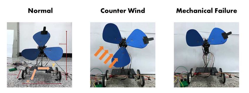
23 Experiments
ble 3 describes characteristics of five models according
24 An experimental apparatus is a three-blade fan on the
25 to temporal structure (Temporal), low-pass filtering
wheels with a low-power digital accelerometer made in
26 (Filter), transformation (Transform), and key features
Analog Device (ADXL345 GY-80) installed as shown
27 (Features). Only 1-NN DTW keeps the temporal struc-
in Fig. 8. The dimension of the apparatus is the width
28 ture of data, and the others do not consider the order
18.5 mm, length of 12.3 mm, and height of 30 mm. For
29 of data points over time. Algorithms for feature extrac-
classification, we considered three of the most probable
30 tion are χ2 test for WEASEL MUSE, Term-Frequency
states of the fan we can think of in a real-world situ-
31 Inverse Document Frequency algorithm for BOSS VS,
ation: The normal state where the fan running with-
32 Entropy for RF, the cost function for LR, and Eu-
out any noticeable event (see left pane in Fig. 8), the
33 clidean distance for 1-NN DTW.
34 counter-wind state in which occurrence of intermit-
35 tency of counter-wind against the fan takes place (see Classification with BOSS VS
36 center pane in Fig. 8), and the mechanical failure state Table 4 shows the numerical expression of the trained
37 where one of the blades is broken off (see right pane model p(C|T) in Table 1, which is the result of vector
38 in Fig. 8). The average rotational speed of the fan was tfidf(S, C) calculated using training data. The sym-
39 114 rpm at normal state, 41 rpm at counter-wind state, bolic algorithm SFA converts the whole training data
40 and 107 rpm at mechanical-failure state, respectively. to S = {aa, ab, ba, bb}. For example, the features of
41 Each sample was collected at a sampling rate of the normal state (C1 ) are aa, ab, ba, and bb with
42 100 Hz for 3 seconds from the accelerometer, so the
43 the numerical values (3.5649, 3.5649, 3.5649, 3.6390)
length of each sample is 300. For example, 900 sam- as displayed in Table 4. For the counter-wind state
44 ples for each state of the fan were collected via x
45 (C2 ), the value reads (3.1972, 2.9459, 3.3025, 3.3025),
and y channels, so the number of data points sums which is clearly distinguished from those of the normal
46
900 samples × 2 channels × 300 × 3 states = 1, 620, 000. state.
47
48 It took 2 hours and 15 minutes for collecting 1,620,000 Table 5 shows the classifier p(C|Q) in Table 1 for
49 of data points at each measurement. The samples of Q. For example, the first sample Q1 is predicted as
50 the experimental data are shown as a set of time series the normal state because of the largest value of 0.9990
51 along with mean and strandard deviation into three throughout the column to which it belongs. In the
52 states in Fig.9. same fashion, the classification is performed for the
53 remaining time series such as the counter-wind state
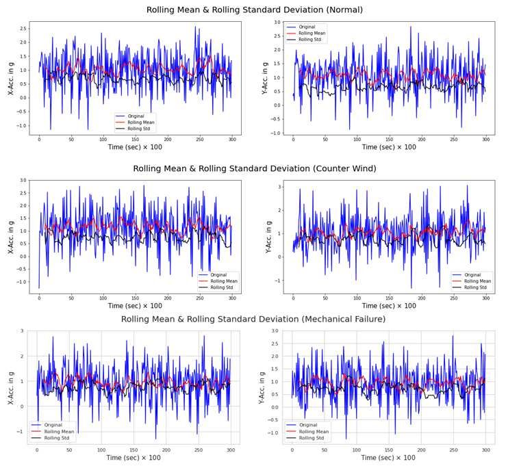
54 Exploratory Data Analysis for Q2 , and the mechanical failure state for Q5 and so
55 Exploratory Data Analysis (EDA) is carried out to on.
56 identify the property of data. In Fig. 9, the raw data,
57 its rolling mean, and the standard deviation are over- Post-Hoc Analysis
58 laid. Since raw data contains much noise, it is neces- Often in many studies, the results tend to be presented
59
sary to filtered out for a better analysis. The rolling without statistical rigor. However, it is important to
60
mean is one such filtering tool. The standard deviation check if it being statistically significant before further
61
62 can be used for estimating variance of data. discussion, which is called Post-Hoc analysis.
63
64
65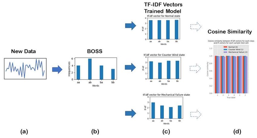
Choi                                                                                                      Page 6 of 11
 1
 2
 3
 4
 5
 6      As shown in Table 6, the BOSS VS model indicates         model are proven statistically significant at a 95% con-
 7   the highest accuracy for all data sizes. In addition,       fidence level. Figure 10 shows yet another aspect of
 8   even though the number of data is increased from 180        the trend of accuracy over run time for all five models,
 9   k to 1.6 million, it shows a little change in accuracy,     where the BOSS VS model outputs a far great perfor-
10   so we may conclude that the BOSS VS model is not            mance in both accuracy and run time.
11   significantly affected by the size of data. The smaller
12   the number of data used, the shorter the run time,          Scalability
13   but on the other hand, the model tends to be over-          In general, a scalable model shows consistently good
14   fitted to the data. For example, in scenario I, 180,000     performance despite an increase in the amount of data.
15   data points was used; for the BOSS VS model, the            Multiple comparisons of run time for five models are
16   accuracy turned out 100%. This can clearly indicates        summarized in Table 9. All pairwise cases for 1-NN
17   overfitting, where too little data was used for training.   DTW model vs the other models turn out to be signif-
18   If the number of data is increased, the time for pre-       icant. Thus, we may conclude that 1-NN DTW model
19   processing and calculation also increases accordingly.      is far less scalable. Figure 11 shows the scalability of
20   Therefore, it is necessary to manipulate the data size      models in which except the 1-NN DTW model the
21                                                               other models keep relatively small changes in the run-
     so that Fog computing may handle a whole process
22
     within a designated time. In this study, we put a time      time subject to increasing data size. Figure 12 shows
23
     limit on the simulation, where the processing time tM L     the comparison of the 95% confidence interval (CI) of
24
25   does not exceed 1/10 of the data collection time tobs .     accuracy of each model using experimental data of dif-
26      Table 6 does not tell whether the difference in the      ferent sizes. The accuracy of the BOSS VS model fell
27   accuracy of each model is statistically meaningful. An-     into CI = 0.9872±0.0073, of which statistical behavior
28   other ambiguity arises in the results of the run time.      is much better compared to CI = 0.8205 ± 0.1319 in
29   Thus, we carried out the ANOVA (Analysis of Vari-           the second-place RF model. Moreover, the deviation
30   ance) test that provides statistical significance among     0.0073 of the BOSS VS model is quite small compared
31   differences. Table 7 shows the ANOVA test result for        to 0.1319 that of the RF model. This explains good
32   accuracy with F = 60.8, and p-value ≤ 0.05 at a 95%         scalability, which indicates that the BOSS VS model
33   confidence level. This indicates that the null hypothe-     is robust to changes in data size.
34   sis is rejected. Therefore, it can be said that the mean
35   values for the accuracy of each model differ signifi-       Conclusion
36   cantly. In addition, the difference in run time for each    Analyzing a huge amount of data transmitted in real
37   model is statistically significant, with F = 4.58, and      time from a networked IoT device, which is a core of
38   p-value = 0.008. In conclusion, the simulation over five    smart manufacturing, to properly classify the state of
39   scenarios for accuracy and run time with five models        the device is interesting and practically important. Re-
40
     can be confirmed to be statistically significant.           cently, there has been a growing tendency to solve this
41
        However, the ANOVA test results shown in Table 7         problem not only in cloud computing but rather at Fog
42
43   alone cannot tell which model is different in accuracy      computing close to IoT devices. To this end, two issues
44   and run time from those of others. Thereby, another         must be resolved: one is is of a cyber-physical model
45   test should be carried out to see which model is signifi-   that can represent the state of an IoT device, and the
46   cantly different from the others. We employed Tukey’s       other is about how to properly process streaming sen-
47   Honest Significant Difference test (Tukey Test) for all     sor data in real-time.
48   pariwise comparisons while controlling multiple com-          A major goal in this study is to build a good cyber-
49   parisons. In this study, the suitability of models was      physical model with significant accuracy in classifica-
50   sought statistically in two aspects: accuracy and scal-     tion. Taking advantage of machine learning and sta-
51   ability.                                                    tistical inference with a vast amount of data, data-
52                                                               driven modeling approach can alienate quite a burden
53   Accuracy                                                    of such complicated theoretical domain-specific knowl-
54   The result of the Tukey Test, which being multiple          edge. While most literature publishes the results of the
55   comparisons of means of accuracy from five models, is       simulation using well-preprocessed public data, in this
56   summarized in Table 8. It is noted that two cases, 1-       study, we implemented noisy real-world data. A three-
57   NN DTW vs WEASEL MUSE and LR vs RF, are not                 blade fan with an accelerometer installed is considered
58
     statistically significant upon a 95% confidance level.      for an IoT device to create a cyber-physical model that
59
     This implies that two cases may have a great simi-          can classify the state of the fan into three states. Using
60
61   larity in the way to make poor predictions. On the          several algorithms including the most recent out ones,
62   contrary, all pairwise comparisons with the BOSS VS         upon the classification performance of five models with
63
64
65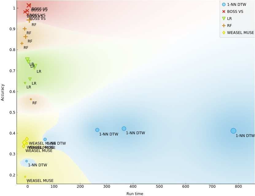
Choi                                                                                                                                             Page 7 of 11
 1
 2
 3
 4
 5
 6   real-world data; we achieved an accuracy of about 98%                              14. Keogh, E., Chakrabarti, K., Pazzani, M., Mehrotra, S.: Dimensionality
     with BOSS VS model.                                                                    reduction for fast similarity search in large time series databases.
 7                                                                                          Knowledge and information Systems 3(3), 263–286 (2001)
 8     For further studies, we need to challenge a cou-                                 15. Salvador, S., Chan, P.: Toward accurate dynamic time warping in linear
 9   ple of tasks for better accuracy and scalability. Thus,                                time and space. Intelligent Data Analysis 11(5), 561–580 (2007)
                                                                                        16. Senin, P., Malinchik, S.: Sax-vsm: Interpretable time series
10   more studies should be conducted for efficient models
                                                                                            classification using sax and vector space model. In: 2013 IEEE 13th
11   and algorithms with machine learning against ever-                                     International Conference on Data Mining, pp. 1175–1180 (2013). IEEE
12   increasing sensors at smart manufacturing, in order
                                                                                        17. Schäfer, P., Högqvist, M.: Sfa: a symbolic fourier approximation and
13   not to wholly depending on cloud computing.
                                                                                            index for similarity search in high dimensional datasets. In: Proceedings
14                                                                                          of the 15th International Conference on Extending Database
15                                                                                          Technology, pp. 516–527 (2012)
     Acknowledgements                                                                   18. Karimi-Bidhendi, S., Munshi, F., Munshi, A.: Scalable classification of
16   The present research was supported by the research fund of Dankook                     univariate and multivariate time series. In: 2018 IEEE International
17   university in 2021.                                                                    Conference on Big Data (Big Data), pp. 1598–1605 (2018). IEEE
18                                                                                      19. Raza, A., Kramer, S.: Accelerating pattern-based time series
     Availability of data and materials
19   Experimental data are included.
                                                                                            classification: a linear time and space string mining approach.
20                                                                                          Knowledge and Information Systems 62(3), 1113–1141 (2020)
     Competing interests                                                                20. Schäfer, P.: The boss is concerned with time series classification in the
21                                                                                          presence of noise. Data Mining and Knowledge Discovery 29(6),
     The authors declare that they have no competing interests.
22                                                                                          1505–1530 (2015)
23   Authors’ information                                                               21. Schäfer, P., Leser, U.: Fast and accurate time series classification with
24   The author is professor of deparment of mechanical engineering at Dankook              weasel. In: Proceedings of the 2017 ACM on Conference on
     University, Korea. His area of research is application of machine learning             Information and Knowledge Management, pp. 637–646 (2017)
25   into smart manufacturing and application on various computing                      22. Wang, Z., Yan, W., Oates, T.: Time series classification from scratch
26   enviroments such as cloud computing, fog computing , and on-device                     with deep neural networks: A strong baseline. In: 2017 International
27   computing.                                                                             Joint Conference on Neural Networks (IJCNN), pp. 1578–1585 (2017).
28                                                                                          IEEE
     References                                                                         23. Karim, F., Majumdar, S., Darabi, H., Chen, S.: Lstm fully
29    1. Kang, H.S., Lee, J.Y., Choi, S., Kim, H., Park, J.H., Son, J.Y., Kim,              convolutional networks for time series classification. IEEE access 6,
30       B.H., Do Noh, S.: Smart manufacturing: Past research, present                      1662–1669 (2017)
31       findings, and future directions. International journal of precision            24. Schäfer, P.: Scalable time series classification. Data Mining and
         engineering and manufacturing-green technology 3(1), 111–128 (2016)                Knowledge Discovery 30(5), 1273–1298 (2016)
32
                                                                                        25. Hatami, N., Gavet, Y., Debayle, J.: Bag of recurrence patterns
33    2. Herrmann, C., Schmidt, C., Kurle, D., Blume, S., Thiede, S.:                       representation for time-series classification. Pattern Analysis and
34       Sustainability in manufacturing and factories of the future.                       Applications 22(3), 877–887 (2019)
35       International Journal of precision engineering and manufacturing-green
         technology 1(4), 283–292 (2014)                                                Figures
36    3. Manyika, J., Chui, M., Bisson, P., Woetzel, J., Dobbs, R., Bughin, J.,
37       Aharon, D.: Unlocking the potential of the internet of things.
38       McKinsey Global Institute (2015)                                                 Figure 1 Three levels of IoT system. As the top-level, IoT
      4. Mohammadi, M., Al-Fuqaha, A., Sorour, S., Guizani, M.: Deep                      employing cloud system associated with big data analytics.
39
         learning for iot big data and streaming analytics: A survey. IEEE                Fog computing resides in the middle equipped with fast
40       Communications Surveys Tutorials 20(4), 2923–2960 (2018)                         streaming data analytics. At the bottom level, IoT devices
41    5. Bonomi, F., Milito, R., Zhu, J., Addepalli, S.: Fog computing and its            such as sensors are located with consecutive temporal data
42       role in the internet of things. In: Proceedings of the First Edition of          requiring real-time data analytics.
         the MCC Workshop on Mobile Cloud Computing, pp. 13–16 (2012)
43    6. Dastjerdi, A.V., Buyya, R.: Fog computing: Helping the internet of
44       things realize its potential. Computer 49(8), 112–116 (2016)
45    7. Stojmenovic, I., Wen, S.: The fog computing paradigm: Scenarios and
46       security issues. In: 2014 Federated Conference on Computer Science
         and Information Systems, pp. 1–8 (2014). IEEE                                    Figure 2 The workflow of Fog computing in the present study.
47    8. Yi, S., Hao, Z., Qin, Z., Li, Q.: Fog computing: Platform and                    Fog computing is composed of three distinctive modes in a
48       applications. In: 2015 Third IEEE Workshop on Hot Topics in Web                  single time sequence: observation, machine learning, and
49       Systems and Technologies (HotWeb), pp. 73–78 (2015). IEEE                        status update. Observation phase executes streaming data
50    9. Gassais, R., Ezzati-Jivan, N., Fernandez, J.M., Aloise, D., Dagenais,            storing. Machine Learning phase does data processing and
         M.R.: Multi-level host-based intrusion detection system for internet of          learning the model. Status update phase carries out a
51       things. Journal of Cloud Computing 9(1), 1–16 (2020)                             classification of a fan status with the trained model. A red box
52   10. Zatwarnicki, K.: Two-level fuzzy-neural load distribution strategy in            refers to a sliding window corresponding to a process of the
53       cloud-based web system. Journal of Cloud Computing 9(1), 1–11                    workflow on the timeline. For example, the box which is on the
54       (2020)                                                                           second from the left indicatese data storing. Likewise, the fifth
     11. Oks, S.J., Jalowski, M., Fritzsche, A., Möslein, K.M.: Cyber-physical           box from the left is of learning the model.
55       modeling and simulation: A reference architecture for designing
56       demonstrators for industrial cyber-physical systems. Procedia CIRP 84,
57       257–264 (2019)
     12. Xu, Z., Zhang, Y., Li, H., Yang, W., Qi, Q.: Dynamic resource
58
         provisioning for cyber-physical systems in cloud-fog-edge computing.
59       Journal of Cloud Computing 9(1), 1–16 (2020)
60   13. Žliobaitė, I., Bifet, A., Read, J., Pfahringer, B., Holmes, G.: Evaluation
61       methods and decision theory for classification of streaming data with
         temporal dependence. Machine Learning 98(3), 455–482 (2015)
62
63
64
65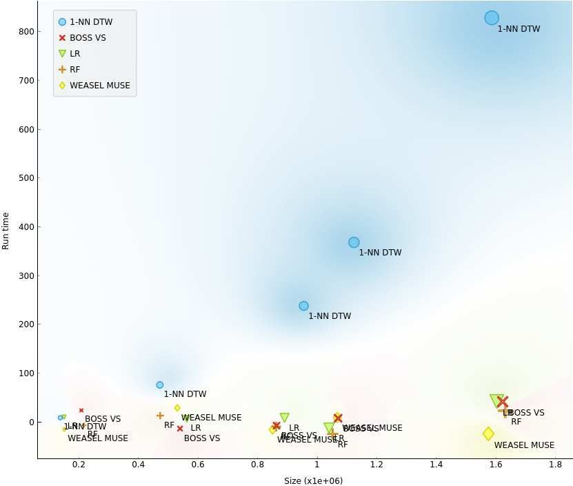
Choi                                                                                                                    Page 8 of 11
 1
 2
 3
 4
 5
 6    Figure 3 A cyber-physical model is expected to well explain
 7    the effect of real-world elements such as acoustic noise,
      mechanical failure, temperatue change, revolution (rpm),
 8    pressure distribution of blades, vibration, counter-wind
 9    occurence, and wind velocity etc.
10
11
12    Figure 4 Low-pass filtering and smoothing of a sample of
13    acceleration in x-axis upon Discrete Fourier Transform (DFT).
14    In this plot, DFT result is obtained by taking only first two
15    Fourier coefficients.
16
17                                                                      Figure 11 Scalability comparison of five models. As the
18    Figure 5 A pictorial diagram of symbolic Fourier                  amount of data is increased, the 1-NN-DTW model shows the
      approximation (SFA) procedure: a) Incoming sensor data of six     worst scalability. On the contrary, the other models show
19    time-series, b) The data is then transformed via Fourier          reasonable scalability. The BOSS VS model performs excellent
20    transform, c) The Fourier coefficients are quantizied via         scalability yet keeping the best accuracy.
21    Multiple Coefficient Binning (MCB), and d) Each time series
22    has been mapped into its respective SFA word.
23
24
25    Figure 6 BOSS model and BOSS VS: a) Samples are being
26    scanned with a sliding window, b) multiple windowed
      subsequences are generated, c) all of the subsequences are
27    transformed into SFA words, d) SFA words are summarized in
28    the form of BOSS histogram (BOSS model), and e) the BOSS
29    histogram is vectorized through Term Frequency Inverse
30    Document Frequency (TF-IDF) model, which finally results in
      TF-IDF vectors for training data.
31
32
33
34    Figure 7 Schematic diagram of classification with the consine
      similarity: a) New data for query is first transformed into SFA
35    words, b) the SFA words of the new data is tranformed into
36    the BOSS histogram, c) the trained model in the form of tf-idf
37    algorithm is given, and d) the classificaiton is carried out
38    through calculating the cosine similarity between the trained
      model and the query.
39
40
41
42    Figure 8 Photos of the three-blade fan in the three states:
      Normal state (left), Counter-wind state (center), and
43    Mechanical failure state (right). The counter-wind state
44    indicates the state where counter-wind being blown by another
45    fan in front of the fan. The mechanical failure refers to the
46    state in which one of the blades having been removed off.         Figure 12 The result of comparing the 95% confidence
                                                                        interval (CI) of the accuracy of five models using five scenarios
47                                                                      of data size. This illustates the scalability of each model’s
48                                                                      performance in classification. The accuracy of the BOSS VS
49    Figure 9 Experimental time series data for three states of the    model fell into CI = 0.9872 ± 0.0073 resulting in the best
50    fan: Normal state (top row), counter-wind state (middle row),     performance.
      and mechanical failure state (bottom row). Raw data from the
51    accelerometer overlaid with the rolling mean and standard
52    deviation. Each row represents both x (left) and y (right)
53    acceleration in g unit.
54
55
56    Figure 10 Accuracy comparison of five models (WEASEL
57    MUSE, BOSS VS, Random Forest, Logistic Regression, and
58    1-Nearest-Neighbor DTW). 1-NN DTW model shows the
      worst performance both in accuracy and run time. On the
59    contrary, the BOSS VS model shows excellent accuracy over
60    the others. Note: the upper left being the overall best
61    performance.
62
63
64
65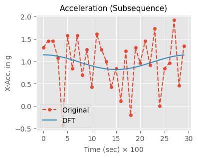
Choi                                                                                                                                  Page 9 of 11
 1
 2
 3
 4
 5
     Tables
 6
 7   Table 1 Lookup table for the probabilistic models and corresponding algorithms.
 8
                              Probability      p(T|C)         p(C)                 p(C|T)                 p(Q|C)              p(C|Q)
 9
10                             Algorithm      tf(S, C)      idf(S, C)         tfidf(S, C)                tf(Q, C)        CosSim(Q, C)
11                               Note           Model          Prior         Trained Model              Transformed           Classifier
12
13
14   Table 2 Augmented Dickey-Fuller (ADF) Test Results: The results show that all of six time-series are found to be stationary of being
15   statistically significant owing to p-value ≤ 0.05 (95% confidence level), which indicates evidence against the null hypothesis H0 .
16
                                            Time Series              ADF statistic                P-value        Critical Value (5%)
17
18                                      x-acc (Normal)                        -4.629        1.1 ×   10−4                       -2.871
                                        y-acc (Normal)                        -6.137        8.1 × 10⁻⁸                         -2.871
19                                  x-acc (Counter Wind)                      -6.486        1.2 × 10⁻⁸                         -2.871
20                                  y-acc (Counter Wind)                      -5.839        3.8 × 10⁻⁷                         -2.871
21                                x-acc (Mechanical Failure)                  -4.577        1.4 × 10⁻⁴                         -2.871
22                                y-acc (Mechanical Failure)                  -4.459        2.3 × 10⁻⁴                         -2.871
23
24
25   Table 3 Comparison of characteristics of five models via conducting normalization (Norm.), keeping temporal structure (Temporal),
26   carrying out low-pass filtering (Filter), executing transformation (Transform), and key features (Features).
27                                                            Temporal        Filter       Transform               Features
28
                                        WEASEL MUSE                 No            Yes            Yes             χ2 test
29                                        BOSS VS                   No            Yes            Yes         Term Frequency
30                                          RF                      No            No             No             Entropy
31                                          LR                      No            No             No               Cost
32                                       1-NN DTW                   Yes           No             No             Distance
33
34
35   Table 4 The trained model p(C|T) with equivalent of TF-IDF vector tfidf(S, C) for the training data. S = {aa, ab, ba, bb} is the
     SFA words and C = {C1 , C2 , C3 } is three states of the fan.
36
37                                              Class        C1               C2                          C3
38                                                         Normal         Counter Wind        Mechanical Failure
39
                                                 aa        3.5649            3.1972                      2.9459
40                                               ab        3.5649            2.9459                      2.3862
41                                               ba        3.5649            3.3025                      2.0986
42                                               bb        3.6390            3.3025                      2.3862
43
44
45   Table 5 The classifier p(C|Q) with equivalent to Cosine similarity between the trained model p(C|T) for each class and new samples
46   Q = {Q1 , . . . , Q6 } as a query. C = {C1 , C2 , C3 } is three states of the fan. The similarity resutls in the prediction for the new samples.
     The maximum value of the cosine similarity for each sample is boldfaced.
47
48                                                            Q1             Q2             Q3             Q4           Q5            Q6
49                                  Normal                0.9990        0.9958           0.9987        0.9963       0.9943       0.9970
50                               Counter Wind              0.9964      0.9977           0.9988          0.9942      0.9909      0.9991
51                              Mechanical Failure         0.9908       0.9791           0.9924         0.9855     0.9985        0.9868
52
53
54
55
56
57
58
59
60
61
62
63
64
65
Choi Page 10 of 11
1
2
3
4
5 Table 6 Comparison of performace of five models according to five scenarios: The number of data points is increased from 180k up to
6 1.6 Million. As for Fog computing: The processor: Intel Core i3-8100 CPU 3.60GHz at 4GB memory, and the OS being Ubuntu 20.04.1
LTS. BOSS VS model shows excellent scalability while keeping the highest accuracy among the other models.
7
8 Scenario Data points (samples) Model tobs (sec) tM L (sec) Accuracy
9 WEASEL MUSE 900 0.398 0.200
10 BOSS VS 900 0.464 1.000
11 I 180,000 (300) RF 900 0.443 0.567
LR 900 0.253 0.633
12 1-NN DTW 900 10.409 0.266
13 WEASEL MUSE 2,700 1.009 0.333
14 BOSS VS 2,700 1.422 0.977
15 II 540,000 (900) RF 2,700 1.163 0.822
LR 2,700 2.540 0.655
16 1-NN DTW 2,700 89.546 0.377
17 WEASEL MUSE 4,500 1.810 0.346
18 BOSS VS 4,500 2.456 0.986
19 III 900,000 (1,500) RF 4,500 1.961 0.906
LR 4,500 7.153 0.740
20 1-NN DTW 4,500 246.794 0.400
21 WEASEL MUSE 5,400 2.193 0.366
22 BOSS VS 5,400 2.966 0.983
23 IV 1,080,000 (1,800) RF 5,400 2.472 0.877
LR 5,400 12.921 0.766
24 1-NN DTW 5,400 352.067 0.411
25 WEASEL MUSE 8,100 3.851 0.370
26 BOSS VS 8,100 4.667 0.988
27 V 1,620,000 (2,700) RF 8,100 3.910 0.929
LR 8,100 32.183 0.711
28 1-NN DTW 8,100 793.221 0.388
29
30 Table 7 ANOVA test result of accuracy and run time among five models.
31 sumsq df F PR(>F)
32
Algorithms (Accuracy) 1.64 4.0 60.80 6.56 × 10⁻¹¹
33 Residual 0.13 20.0 - -
34
Algorithms (Run time) 346268.91 4.0 4.58 0.008631
35 Residual 377628.33 20.0 - -
36
37 Table 8 Multiple Comparison of Means of Accuracy - Tukey HSD test
38
39 Group1 Group2 meandiff p-adj lower upper reject
40 1-NN DTW BOSS VS 0.614 0.001 0.458 0.770 True
41 1-NN DTW LR 0.328 0.001 0.172 0.484 True
1-NN DTW RF 0.447 0.001 0.292 0.603 True
42 1-NN DTW WEASEL MUSE -0.049 0.862 -0.205 0.106 False
43 BOSS VS LR -0.286 0.001 -0.441 -0.130 True
44 BOSS VS RF -0.166 0.032 -0.322 -0.011 True
45 BOSS VS WEASEL MUSE -0.663 0.001 -0.819 -0.508 True
LR RF 0.119 0.187 -0.036 0.274 False
46 LR WEASEL MUSE -0.377 0.001 -0.533 -0.222 True
47 RF WEASEL MUSE -0.497 0.001 -0.652 -0.341 True
48
49 Table 9 Multiple Comparison of Means of run time - Tukey HSD
50 Group1 Group2 meandiff p-adj lower upper reject
51
1-NN DTW BOSS VS -296.01 0.020 -556.08 -35.93 True
52 1-NN DTW LR -287.39 0.025 -547.47 -27.32 True
53 1-NN DTW RF -296.41 0.020 -556.49 -36.34 True
54 1-NN DTW WEASEL MUSE -296.55 0.020 -556.62 -36.48 True
55 BOSS VS LR 8.61 0.900 -251.45 268.68 False
BOSS VS RF -0.405 0.900 -260.47 259.66 False
56 BOSS VS WEASEL MUSE -0.542 0.900 -260.61 259.53 False
57 LR RF -9.02 0.900 -269.09 251.05 False
58 LR WEASEL MUSE -9.15 0.900 -269.23 250.91 False
59 RF WEASEL MUSE -0.137 0.900 -260.21 259.93 False
60
61
62
63
64
65Choi Page 11 of 11
1
2
3
4
5
Additional Files
6 Additional files
7 Experimental Raw Data file (statef an.csv)
8 All figure files
9
10
11
12
13
14
15
16
17
18
19
20
21
22
23
24
25
26
27
28
29
30
31
32
33
34
35
36
37
38
39
40
41
42
43
44
45
46
47
48
49
50
51
52
53
54
55
56
57
58
59
60
61
62
63
64
65Figures Figure 1 Three levels of IoT system. As the top-level, IoT employing cloud system associated with big data analytics. Fog computing resides in the middle equipped with fast streaming data analytics. At the bottom level, IoT devices such as sensors are located with consecutive temporal data requiring real-time data analytics.
Figure 2

The work ow of Fog computing in the present study. Fog computing is composed of three distinctive
modes in a single time sequence: observation, machine learning, and status update. Observation phase
executes streaming data storing. Machine Learning phase does data processing and learning the model.
Status update phase carries out a classi cation of a fan status with the trained model. A red box refers to
a sliding window corresponding to a process of the work ow on the timeline. For example, the box which
is on the second from the left indicatese data storing. Likewise, the fth box from the left is of learning
the model.
Figure 3

A cyber-physical model is expected to well explain the effect of real-world elements such as acoustic
noise, mechanical failure, temperatue change, revolution (rpm), pressure distribution of blades, vibration,
counter-wind occurence, and wind velocity etc.

Figure 4

Low-pass ltering and smoothing of a sample of acceleration in x-axis upon Discrete Fourier Transform
(DFT). In this plot, DFT result is obtained by taking only rst two Fourier coe cients.
Figure 5

A pictorial diagram of symbolic Fourier approximation (SFA) procedure: a) Incoming sensor data of six
time-series, b) The data is then transformed via Fourier transform, c) The Fourier coe cients are
quantizied via Multiple Coe cient Binning (MCB), and d) Each time series has been mapped into its
respective SFA word.
Figure 6

BOSS model and BOSS VS: a) Samples are being scanned with a sliding window, b) multiple windowed
subsequences are generated, c) all of the subsequences are transformed into SFA words, d) SFA words
are summarized in the form of BOSS histogram (BOSS model), and e) the BOSS histogram is vectorized
through Term Frequency Inverse Document Frequency (TF-IDF) model, which nally results in TF-IDF
vectors for training data.
Figure 7

Schematic diagram of classi cation with the consine similarity: a) New data for query is rst transformed
into SFA words, b) the SFA words of the new data is tranformed into the BOSS histogram, c) the trained
model in the form of tf-idf algorithm is given, and d) the classi caiton is carried out through calculating
the cosine similarity between the trained model and the query.

Figure 8

Photos of the three-blade fan in the three states: Normal state (left), Counter-wind state (center), and
Mechanical failure state (right). The counter-wind state indicates the state where counter-wind being
blown by another fan in front of the fan. The mechanical failure refers to the state in which one of the
blades having been removed off.

Figure 9

Experimental time series data for three states of the fan: Normal state (top row), counter-wind state
(middle row), and mechanical failure state (bottom row). Raw data from the accelerometer overlaid with
the rolling mean and standard deviation. Each row represents both x (left) and y (right) acceleration in g
unit.
Figure 10

Accuracy comparison of ve models (WEASEL MUSE, BOSS VS, Random Forest, Logistic Regression, and
1-Nearest-Neighbor DTW). 1-NN DTW model shows the worst performance both in accuracy and run time.
On the contrary, the BOSS VS model shows excellent accuracy over the others. Note: the upper left being
the overall best performance.
Figure 11

Scalability comparison of ve models. As the amount of data is increased, the 1-NN-DTW model shows
the worst scalability. On the contrary, the other models show reasonable scalability. The BOSS VS model
performs excellent scalability yet keeping the best accuracy.
Figure 12

The result of comparing the 95% con dence interval (CI) of the accuracy of ve models using ve
scenarios of data size. This illustates the scalability of each model's performance in classi cation. The
accuracy of the BOSS VS model fell into CI = 0:9872 ± 0:0073 resulting in the best performance.

Supplementary Files
This is a list of supplementary les associated with this preprint. Click to download.

    statefan.csv
You can also read