MARSBAR DOCUMENTATION - RELEASE 0.44 MATTHEW BRETT
←
→
Page content transcription
If your browser does not render page correctly, please read the page content below
MarsBaR Documentation
             Release 0.44

            Matthew Brett

                Sep 25, 2021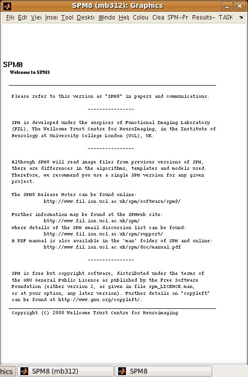
CONTENTS

1   About MarsBaR                                                                                                                                                                                  3
    1.1 Citing MarsBaR . . . . . . . . . . . . . . . . . . . . . . . . . . . . . . . . . . . . . . . . . . . . .                                                                                   3
    1.2 Thanks . . . . . . . . . . . . . . . . . . . . . . . . . . . . . . . . . . . . . . . . . . . . . . . . . .                                                                                 3

2   Download and install                                                                                                                                                                           5
    2.1 Installing MarsBaR . . . . . . . . . . . . . . . . . . . . . . . . . . . . . . . . . . . . . . . . . . . .                                                                                 5
    2.2 Other MarsBaR downloads . . . . . . . . . . . . . . . . . . . . . . . . . . . . . . . . . . . . . . .                                                                                      6

3   MarsBaR tutorial                                                                                                                                                                               7
    3.1 Getting started . . . . . . . .   .   .   .   .   .   .   .   .   .   .   .   .   .   .   .   .   .   .   .   .   .   .   .   .   .   .   .   .   .   .   .   .   .   .   .   .   .   .    7
    3.2 The MarsBaR / SPM interface       .   .   .   .   .   .   .   .   .   .   .   .   .   .   .   .   .   .   .   .   .   .   .   .   .   .   .   .   .   .   .   .   .   .   .   .   .   .    9
    3.3 Defining ROIs . . . . . . . .     .   .   .   .   .   .   .   .   .   .   .   .   .   .   .   .   .   .   .   .   .   .   .   .   .   .   .   .   .   .   .   .   .   .   .   .   .   .   13
    3.4 Running the ROI analysis . .      .   .   .   .   .   .   .   .   .   .   .   .   .   .   .   .   .   .   .   .   .   .   .   .   .   .   .   .   .   .   .   .   .   .   .   .   .   .   19
    3.5 Basic results . . . . . . . . .   .   .   .   .   .   .   .   .   .   .   .   .   .   .   .   .   .   .   .   .   .   .   .   .   .   .   .   .   .   .   .   .   .   .   .   .   .   .   23
    3.6 Using a structural ROI . . . .    .   .   .   .   .   .   .   .   .   .   .   .   .   .   .   .   .   .   .   .   .   .   .   .   .   .   .   .   .   .   .   .   .   .   .   .   .   .   28
    3.7 Batch mode . . . . . . . . . .    .   .   .   .   .   .   .   .   .   .   .   .   .   .   .   .   .   .   .   .   .   .   .   .   .   .   .   .   .   .   .   .   .   .   .   .   .   .   29
    3.8 The end . . . . . . . . . . . .   .   .   .   .   .   .   .   .   .   .   .   .   .   .   .   .   .   .   .   .   .   .   .   .   .   .   .   .   .   .   .   .   .   .   .   .   .   .   29

4   MarsBaR FAQ                                                                                                                                                                                   31
    4.1 What’s with the fish? . . . . . . . . . . . . . . . . . . . . . . . . . . . . . . . . . . . . .                                                                   .   .   .   .   .   .   31
    4.2 Why do I get an error “Cant open image file” when estimating a design? . . . . . . . . .                                                                          .   .   .   .   .   .   31
    4.3 How is the percent signal change calculated? . . . . . . . . . . . . . . . . . . . . . . . .                                                                      .   .   .   .   .   .   32
    4.4 How do I run a MarsBaR analysis in batch mode? . . . . . . . . . . . . . . . . . . . . .                                                                          .   .   .   .   .   .   33
    4.5 How can I extract the percent of activated voxels from an ROI? . . . . . . . . . . . . . .                                                                        .   .   .   .   .   .   34
    4.6 How do I get timecourses from images in an SPM design? . . . . . . . . . . . . . . . . .                                                                          .   .   .   .   .   .   34
    4.7 I just want to get raw timecourses from some images; how do I do that? . . . . . . . . . .                                                                        .   .   .   .   .   .   34
    4.8 I get errors using the SPM ReML estimation for FMRI designs. Can I try something else?                                                                            .   .   .   .   .   .   35
    4.9 How is the FIR (or PSTH) calculated? . . . . . . . . . . . . . . . . . . . . . . . . . . . .                                                                      .   .   .   .   .   .   35
    4.10 How do I extract all the FIR timecourses from my design? . . . . . . . . . . . . . . . . .                                                                       .   .   .   .   .   .   35
    4.11 How do I extract percent signal change from my design using batch? . . . . . . . . . . .                                                                         .   .   .   .   .   .   36
    4.12 How do I do a random effect analysis in MarsBaR? . . . . . . . . . . . . . . . . . . . . .                                                                       .   .   .   .   .   .   36
    4.13 Should I use MarsBaR ROI analysis, or small volume correction (SVC) in SPM? . . . . .                                                                            .   .   .   .   .   .   37
    4.14 Should I use smoothed or unsmoothed images for my MarsBaR analysis? . . . . . . . . .                                                                            .   .   .   .   .   .   37
    4.15 Why can’t I select files like SPM designs in the matlab GUI? . . . . . . . . . . . . . . . .                                                                     .   .   .   .   .   .   38
    4.16 Why do I get a “No valid data for roi” warning when extracting data? . . . . . . . . . . .                                                                       .   .   .   .   .   .   38

5   Support                                                                                                                                                                                       39

6   Reading and writing MarsBaR code                                                                                                                                                              41
    6.1 Getting the latest development code . . . . . . . . . . . . . . . . . . . . . . . . . . . . . . . . . . .                                                                                 41
    6.2 API documentation . . . . . . . . . . . . . . . . . . . . . . . . . . . . . . . . . . . . . . . . . . . .                                                                                 41

                                                                                                                                                                                                   i
7 Indices and tables 43 ii
MarsBaR Documentation, Release 0.44

MarsBaR (MARSeille Boîte À Région d’Intérêt) is a toolbox for SPM which provides routines for region of interest
analysis. Features include region of interest definition, combination of regions of interest with simple algebra, extrac-
tion of data for regions with and without SPM preprocessing (scaling, filtering), and statistical analyses of ROI data
using the SPM statistics machinery.

CONTENTS                                                                                                               1
MarsBaR Documentation, Release 0.44

2                                     CONTENTS
CHAPTER

                                                                                                          ONE

                                                                                       ABOUT MARSBAR

1.1 Citing MarsBaR

We presented an abstract to the Human Brain Mapping conference for 2002; this may be useful as a reference: Mars-
BaR HBM abstract. It should apparently be cited as:
      Matthew Brett, Jean-Luc Anton, Romain Valabregue, Jean-Baptiste Poline. Region of interest analysis
      using an SPM toolbox [abstract] Presented at the 8th International Conference on Functional Mapping of
      the Human Brain, June 2-6, 2002, Sendai, Japan. Available on CD-ROM in NeuroImage, Vol 16, No 2.

1.2 Thanks

For writing credits and some little jokes, see the marsbar.m file file in the MarsBaR release.

                                                                                                               3
MarsBaR Documentation, Release 0.44 4 Chapter 1. About MarsBaR
CHAPTER

                                                                                                              TWO

                                                                        DOWNLOAD AND INSTALL

All MarsBaR file releases are available via the MarsBaR project download page.

2.1 Installing MarsBaR

MarsBaR needs a version of SPM, so if you don’t have SPM, please download and install that first. MarsBaR works
with SPM versions 99, 2, 5, and 8.
For the current stable release of MarsBaR, look for the marsbar package; marsbar-devel is the development release.
Releases consist of an archive which will unpack in a directory named after the MarsBaR version - for example
marsbar-0.42. You then have two options for using MarsBaR within SPM.
   1. You can add the new MarsBaR directory to your matlab path. To use MarsBaR, start it from the matlab prompt
      with the command “marsbar”, or. . .
   2. You could set up MarsBaR to run as an SPM toolbox. To do this, the contents of the new MarsBaR directory
      needs to be in a subdirectory “marsbar” of the SPM toolbox directory. Here is a worked example for Unix.
      Imagine SPM8 was in /usr/local/spm/spm8, and you had just unpacked the MarsBaR distribution, giving
      you a directory /home/myhome/marsbar-0.42. You could then create the marsbar SPM toolbox directory
      with:

      mkdir /usr/local/spm/spm8/toolbox/marsbar

      and copy the MarsBaR distribution into this directory with:

      cp -r /home/myhome/marsbar-0.42/* /usr/local/spm/spm8/toolbox/marsbar

      Alternatively, you could do the same job by making a symbolic link between the directories with something
      like:

      ln -s /home/myhome/marsbar-0.42 /usr/local/spm/spm8/toolbox/marsbar

Either way, the next time you start spm you should be able to start the toolbox by selecting ‘marsbar’ from the toolbox
button on the SPM interface.

                                                                                                                     5
MarsBaR Documentation, Release 0.44
2.2 Other MarsBaR downloads
2.2.1 Example dataset
You may want the example dataset to try out MarsBaR, or to run the MarsBaR tutorial.
Download the dataset from the MarsBaR project download page.
To install, unpack the archive in a directory you can write to. This will give you a subdirectory like
marsbar_example_data-0.3, where 0.3 is the version number of the example data.
The example data are taken from an experiment described in an HBM2003 conference abstract:
Matthew Brett, Ian Nimmo-Smith, Katja Osswald, Ed Bullmore (2003) Model fitting and power in fast
event related designs. NeuroImage, 19(2) Supplement 1, abstract 791
The data consist of three EPI runs, all from one subject. In each run the subject watched a computer screen, and
pressed a button when they saw a flashing checker board. An “event” in this design is one presentation of the flashing
checker board.
We did this experiment because we were interested to see if events at fast presentation rates give different activation
levels from events that are more widely spaced. Each run has a different presentation rate. We randomized the times
between events in each run to give an average rate of 1 event every second in run 1, 1 event every 3 seconds for run 2,
and 1 event every 10 seconds for run 3.
There are some automated pre-processing scripts for this dataset in the MarsBaR distribution, see Starting the tutorial
for more details.
2.2.2 AAL structural ROIs
These ROIs can be useful as a standard set of anatomical definitions.
To install, download the AAL ROI archive file from the MarsBaR project download page. Unpack the archive some-
where; it will create a new directory, called something like marsbar-aal-0.2.
The AAL ROI library contains ROIs in MarsBaR format that were anatomically defined by hand on a single brain
matched to the MNI / ICBM templates. The ROI definitions are described in:
Tzourio-Mazoyer N, Landeau B, Papathanassiou D, Crivello F, Etard O, Delcroix N, et al. (2002). Au-
tomated anatomical labelling of activations in SPM using a macroscopic anatomical parcellation of the
MNI MRI single subject brain. NeuroImage 15: 273-289.
6 Chapter 2. Download and installCHAPTER
THREE
MARSBAR TUTORIAL
This is a short introduction to MarsBaR, a region of interest toolbox for SPM. It takes the form of a guided tour,
showing the usage of MarsBaR with a standard dataset.
The tutorial assumes you have some experience using SPM
3.1 Getting started
3.1.1 How to read the tutorial
There are three threads in this tutorial. The first and most obvious is a step by step guide to running several standard
ROI analyses. On the way, there are two sets of diversions. These are interface summaries, and technical notes.
Interface summaries look like this:
An interface summary
with some interface description
and technical notes look like this:
A technical note
with some technical notes
If you just want to do the step-by-step tutorial, you can skip these diversions, and come back to them later. The
interface summaries give you information on the range of things that MarsBaR can do; the technical notes are detailed
explanations of the workings of MarsBaR, which can be useful in understanding the obscure parts of the interface.
3.1.2 Gearing up
To run all the examples in this tutorial you will need to download and install two packages:
1. MarsBaR: this tutorial assumes marsbar version 0.44;
2. the example dataset (version 0.3).
To install these packages, see Download and install
This tutorial assumes you are using SPM8, but you can run the tutorial with SPM versions 12, 8, 5, 2 or 99; the results
will be very similar.
7MarsBaR Documentation, Release 0.44 3.1.3 Plan of campaign The Example dataset is from an experiment with three EPI runs of flashing checkerboard events. The first run was at a high presentation rate (average 1 per second), run 2 was at a medium rate (average 1 every 3 seconds) and run 3 was slow (1 every 10 seconds on average). We are going to analyse the data to see if there is different activation for fast and slow presentation rates. ROI analysis is an obvious choice here, because we know where the activation is likely to be – in the primary visual cortex – but we are more interested in how much activation there will be. So, we will first need to define an ROI for the visual cortex, and then analyze the data within the ROI. In this tutorial we will cover two methods of defining an ROI: first, a functional definition and second, an anatomical definition. 3.1.4 Defining a functional ROI A key problem in an ROI analysis is finding the right ROI. This is easier for the visual cortex than for almost any other functional area, because the location of the visual cortex is fairly well predicted by the calcarine sulcus, in the occipital lobe, which is easy enough to define on a structural scan. However, there is a moderate degree of individual variation in the size and border of the primary visual cortex. One approach to this problem is to use the subject’s own activation pattern to define the ROI. We might ask the subject to do another visual task in the scanner, and use SPM to detect the activated areas. We find the subject’s primary visual cortex from the activation map, and use this functional ROI to analyze other data from the same subject. This approach has been very fruitful for areas such as the fusiform face area, which vary a great deal in position between subjects. For this dataset, we are most interested in the difference between the fast presentation rates of run 1, and the slow presentation rates of run 3. So, we can use an SPM analysis of run 2 to define the visual cortex, and use this as an ROI for our analysis of run 1 and run 3. 3.1.5 Functional ROIs usually need independent data Using the recipe above, we are not using run 2 for the ROI analysis. Because we will use run 2 to define the ROI, if we extract data from this ROI for run 2, it will be biased to be more activated than the data from run 1 and run 3. Imagine that our experiment had not worked, and there was no real activation in any of the runs. We do an SPM analysis on run 2, and drop the threshold to find some voxels with higher signal than others due to noise. We define the ROI using this noise cluster, and extract data from the ROI for this session, and the other two sessions. The activation signal from the ROI in run 2 will probably appear to be higher than for the other sessions, because we selected these voxels beforehand to have high signal for run 2. The same argument applies if we select the ROI from a truly activated area; the exact choice of voxels will depend to some extent on the noise in this session, and so data extracted from this ROI, for this session, will be biased to have high signal. 3.1.6 Starting the tutorial First you will need to run some processing on the example dataset. After you unpack the dataset archive, you should have four subdirectories in the main marsbar_example_data directory. Directories sess1, sess2 and sess3 contain the slice-time corrected and realigned, undistorted, spatially normalized data for the three sessions (runs) of the experiment. The rois directory contains pre-defined regions of interest. To run the tutorial, find where your marsbar directory is. You can do this from the matlab prompt with >> which marsbar . If is the marsbar directory, then you should be able to see a directory called / examples/batch. This batch subdirectory contains Matlab program files to run the preprocessing. Change directory to batch, and start Matlab. From the Matlab prompt, run the command run_preprocess. This little script will smooth the images by 8mm FWHM, and run SPM models for each run. 8 Chapter 3. MarsBaR tutorial
MarsBaR Documentation, Release 0.44

Now start MarsBaR. First, make sure the MarsBaR directory is on the Matlab path. If you are using the GUI to add
marsbar to the path, add only the path containing marsbar.m, but not the subdirectories in this directory. Next, run
the command marsbar from the Matlab >> prompt.

3.2 The MarsBaR / SPM interface

Let’s begin by naming the windows used by SPM and MarsBaR. After you have started SPM and MarsBaR, you
should have the following set of windows:
The MarsBaR window:

Then, at the top left of the screen, the SPM buttons window

3.2. The MarsBaR / SPM interface                                                                                  9
MarsBaR Documentation, Release 0.44

Underneath the SPM buttons window, at the bottom left of the screen, is the SPM input window:

SPM and MarsBaR use this window to get input from you, gentle user, such as text, numbers, or menu choices. Usually
on the right hand side of the screen, there is the SPM graphics window:

10                                                                               Chapter 3. MarsBaR tutorial
MarsBaR Documentation, Release 0.44

which is used to display results and other graphics.
When SPM and MarsBaR want file or directory names from you, they may use the file selection window:

3.2. The MarsBaR / SPM interface                                                                      11
MarsBaR Documentation, Release 0.44

Sometimes MarsBaR does not use the SPM selection dialog above, but the standard Matlab dialog, that will differ for
each platform (linux, windows, mac). Here’s a linux version:

12                                                                               Chapter 3. MarsBaR tutorial
MarsBaR Documentation, Release 0.44

3.3 Defining ROIs

The preprocessing script has already run an SPM model for run 2 (and run 1 and run 3). Now we need to find an
activation cluster in the visual cortex.
Go to the MarsBaR window, and click on ROI definition. You should get a menu like this:

Interface summary - the ROI definition menu
View displays one or ROIs on a structural image.
Get SPM cluster(s) uses the SPM results interface to select and save activation clusters as ROIs.
Build gives an interface to various methods for defining ROIs, using shapes (boxes, spheres), activation clusters, and
     binary images.
Transform offers a GUI for combining ROIs, and for flipping the orientation of an ROI to the right or left side of the
     brain.
Import allows you to import all SPM activations as ROIs, or to import ROIs from cluster images, such as those
     written by the SPM results interface, or from images where ROIs are defined by number labels (ROI 1 has value
     1, ROI 2 has value 2, etc.). Similarly
Export writes ROIs as images for use in other packages, such as MRIcro.

3.3.1 Defining a functional ROI

We are going to define the functional ROI using the SPM analysis for run 2. Select Get SPM cluster(s). . . : from the
menu. This runs the standard SPM results interface. Use the file selection window that SPM offers to navigate to the
sess2/SPM8_ana directory. Select the SPM.mat file and click Done. Choose the stim_hrf t contrast from the
SPM contrast manager, click Done. Then accept all the default answers from the interface, like this:

3.3. Defining ROIs                                                                                                 13
MarsBaR Documentation, Release 0.44
Prompt Response
apply masking none
title for comparison stim_hrf
p value adjustment to control none
threshold {T or p value} 0.05
& extent threshold {voxels} 0
Technical note - MarsBaR and SPM designs
For the large majority of tasks, MarsBaR can use SPM designs interchangeably. For example, when running with
SPM5, you can load SPM99 designs and estimate them in MarsBaR; you can also estimate SPM5 designs from
MarsBaR, even if you are using - say - SPM99. However, MarsBaR uses the standard SPM routines for the ‘Get SPM
cluster(s)’ routines. This means that if, for example, you are running SPM5 you can only get clusters from an SPM5
design and you can only get clusters from an SPM99 design if you are running SPM99.
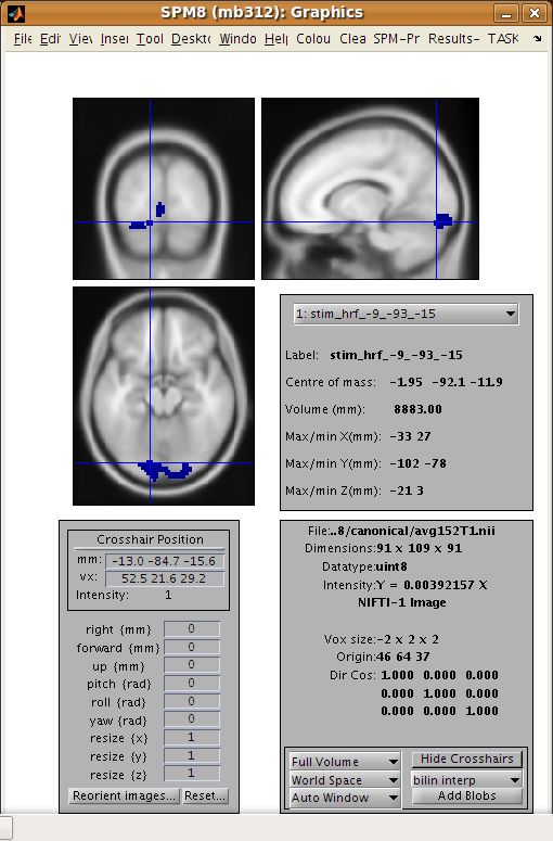
Now you have run the Get SPM cluster(s) interface, you should have an SPM activation map in the graphics window:
Meanwhile, you may have noticed there is a new menu in the SPM input window:
14 Chapter 3. MarsBaR tutorialMarsBaR Documentation, Release 0.44
Another thing you may not have noticed is that the matlab working directory has now changed to the sess2/
SPM8_ana. SPM does this to be able to keep track of where its results files are.
Move the red arrow in the SPM graphics window to the activation cluster in the visual cortex. You can do this by
dragging the arrow, or right-clicking to the right of the axial view and choosing goto global maxima.
When the red arrow is in the main cluster, click on the Write ROI(s) menu in the SPM input window and select Write
one cluster.
Interface summary - Write ROI(s)
Write one cluster writes out a single cluster at the selected location.
Write all clusters writes all clusters from the SPM map; MarsBaR will ask for a directory to save the files, and a root
name for the ROI files before saving each ROI as a separate file.
Rerun results UI restarts the SPM results interface as if you had clicked on the SPM results button; Clear clears the
SPM graphics window.
After you have selected Write one cluster, MarsBaR asks for details to save with the ROI, which are a description, and
a label. Both provide information about the ROI for statistical output and display. The label should be 20 characters or
so, the description can be longer. For the moment, accept the defaults, which derive from the coordinates of the voxel
under the red arrow and the title of the contrast:
Prompt Response
Description of ROI stim_hrf cluster at [-9.0 -93.0 -15.0]
Label for ROI stim_hrf_-9_-93_-15
After this, MarsBaR offers a dialog box to give a filename for the ROI. By default the offered filename will be
stim_hrf_-9_-93_-15_roi.mat in the sess2/SPM8_ana directory. For simplicity, why not accept the
default name and click Save to save the ROI.
Technical note - ROIs and filenames
MarsBaR stores each ROI in a separate file. In fact, the files are in the Matlab .mat format. MarsBaR will accept any
filename for the ROI, and can load ROIs from any file that you have saved them to, but it will suggest that you save the
ROI with a filename that ends in _roi.mat. This is just for convenience, so that when you are asked to select ROIs,
the MarsBaR GUI can assume that ROI files end with this suffix. It will probably make your life easier if you keep to
this convention.
3.3.2 Review the ROI
We can now review this ROI to check if it is a good definition of the visual cortex. Click on the ROI definition menu
in the MarsBaR window, and select View. . . . Choose the ROI and click Done. Your ROI should be displayed in blue
on an average structural image:
3.3. Defining ROIs 15MarsBaR Documentation, Release 0.44 Interface summary - the view utility The view utility allows you to click around the image to review the ROI in the standard orthogonal views. You can select multiple ROIs to view on the same structural. The list box to the left of the axial view allows you to move to 16 Chapter 3. MarsBaR tutorial
MarsBaR Documentation, Release 0.44

a particular ROI (if you have more than one). When the cross-hairs are in the ROI, the information panel will show
details for that ROI, such as centre of mass, and volume in mm. The default structural image is the MNI 152 T1
average brain; you can choose any image to display ROIs on by clicking on the Options. . . menu in the MarsBaR
window, then choosing Edit Options. . . , followed by Default structural.

3.3.3 Refining the ROI

Now we have reviewed the ROI, we see that the cluster does include visual cortex, but there also seems to be some
connected activation lateral and inferior to the primary visual cortex. The cross-hairs in the figure are at something
like the border between primary visual cortex and more lateral voxels. Ideally we would like to restrict the ROI to
voxels in the primary visual cortex.
We can do this by defining a box ROI that covers the area we are interested in, and combining this with the activation
cluster.

Defining a box ROI

To decide on the box dimensions, click around the ROI in the view interface and note the coordinates of the cross-hairs
that are shown at the top of the bottom left panel. This may suggest to you, as it did to us, that it would be good to
restrict the ROI to between -20 and +20mm in X, -66 to -106mm in Y, and -20 to +7mm in Z.
To define this box ROI, click on ROI definition, and choose Build. . . , . You will see a new menu in the SPM input
window:

From the menu, select Box (ranges XYZ). Answer the prompts like this:

3.3. Defining ROIs                                                                                                  17
MarsBaR Documentation, Release 0.44

                  Prompt                   Response
                  [2] Range in X (mm)      -20 20
                  [2] Range in Y (mm)      -66 -106
                  [2] Range in Z (mm)      -20 7
                  Description of ROI       box at -20.0>XYZ
MarsBaR Documentation, Release 0.44 with specified sizes. For example, when MarsBaR combines ROIs, it needs some default space (dimensions, voxel sizes) in which to define the new point list ROI. By default, this is the space of the MNI template; so the Base space for ROIs in the menu above will be MNI space. This is a good space to use if you are working with spatially normalized data, but ROIs are often defined on a subject’s data before spatial normalization. In this case, it may be more useful to set the ROI base space to match the subject’s own activation images, using Options, Edit options from the MarsBaR window. The issue of the ROI space comes up here, because we need to define what dimensions and voxels we should use when writing the image. We can either write the image using the Base space, or we can use some arbitrary space defined by an image, or we can get the space directly from the ROI. Here, the ROI is an activation cluster, and the native ROI space for an activation cluster uses the minimum dimensions necessary to hold all the voxels in the ROI. An ROI image for this cluster using native space uses minimum disk storage, but does not give a good impression of the ROI location when displayed in, for example, MRIcro. In our case, the data are spatially normalized, and so are in the space of the MNI template. The MNI template space is the default base space for ROIs, so select Base space for ROIs, choose a directory to save the image, and accept the default filename for the image, which should be trim_stim. You can check this has worked, by finding the SPM buttons window, selecting Display, and choosing the new trim_stim.img. 3.4 Running the ROI analysis First, let us estimate the activation within the ROI for the first run. There are three stages to the analysis: 1. Choosing the design 2. Extracting the data 3. Estimating the design model with the data The preprocessing for the example data created an SPM model for all three EPI runs, so we already have a design made for the first run. We are going to use this design and the trim_stim ROI to extract ROI data from the functional scans. Then we will use the design and the extracted data to estimate the model. 3.4.1 Stage 1: choosing the design Click on the Design button in the MarsBaR window. You should get a menu like this: 3.4. Running the ROI analysis 19
MarsBaR Documentation, Release 0.44

Interface summary - design menu
The design menu offers options for creating, reviewing, estimating and processing SPM / MarsBaR designs.
Oddly, let us start at the end:
Show default design summary Displays a summary of the currently loaded design in the SPM graphics window
Set design from file will ask for a design file, and load the specified design into MarsBaR. The loaded design then
      becomes the default design. MarsBaR will from now on assume that you want to work with this design, unless
      you tell it otherwise by loading a different design.
Save design to file will save the current default design to a file.
Set design from estimated as we will see later, when MarsBaR estimates a design, it stores the estimated design in
      memory. Sometimes it is useful to take this estimated design and set it to be the default design, in order to be
      able to use the various of these menu options to review the design.
Now, from the top of the menu:
PET models, FMRI models, and Basic models will use the SPM design routines to make a design, and store it in
    memory as the default design.
Explore runs the SPM interface for reviewing and exploring designs.
Frequencies (event+data) can be useful for FMRI designs. The option gives a plot of the frequencies present in ROI
     data and the design regressors for a particular FMRI event. This allows you to choose a high-pass filter that
     will not remove much of the frequencies in the design, but will remove low frequencies in the data, which are
     usually dominated by noise.
Add images to FMRI design allows you to specify images for an FMRI design that does not yet contain images.
     SPM and MarsBaR can create FMRI designs without images. If you want to extract data using the design (see
     below), you may want to add images to the design using this menu item.

20                                                                                  Chapter 3. MarsBaR tutorial
MarsBaR Documentation, Release 0.44
Add/edit filter for FMRI design gives menu options for specifying high pass and possibly (SPM99) low-pass filters,
as well as autocorrelation options (SPM2 and later).
Check images in the design looks for the images names in a design, and simply checks if they exist on the disk,
printing out a message on the matlab console window. A common problem in using saved SPM designs is that
the images specified in the design have since moved or deleted; this option is a useful check to see it that has
occurred.
Change path to images allows you to change the path of the image filenames saved in the SPM design, to deal with
the situation when images have moved since the design was saved.
Convert to unsmoothed takes the image names in a design, and changes them so that they refer to the unsmoothed
version of the same images – in fact it just removes the “s” prefix from the filenames. This can be useful when
you want to use an SPM design that was originally run on smoothed images, but your ROI is very precise, so
you want to avoid running the ROI analysis on smoothed data, which will blur unwanted signal into your ROI.
If you have been reading the interface summary, welcome back. Isn’t it strange how time just seems to stop when you
are reading about graphical user interfaces?
Our plan was to choose our design. Select the Set design from file option in the design menu and choose the SPM.mat
file in the sess1/SPM8_ana directory. MarsBaR loads the design into memory and displays the design matrix in
the SPM graphics window.
3.4.2 Stage 2: extracting the data
Before we can run the model, we need to extract the ROI data from the functional scans. This brings us to the data
menu:
We are going to choose Extract ROI data(default), and for simple analyses this may be all you will ever need. For
those with a thirst for knowledge, here is the:
3.4. Running the ROI analysis 21MarsBaR Documentation, Release 0.44
Interface summary - data menu
Extract ROI data (default) takes one or more ROI files and a design, and extracts the data within the ROI(s) for all
the images in the design. As for the default design, MarsBaR stores the data in memory for further use.
Extract ROI data (full options) allows you to specify any set of images to extract data from, and will give you a full
range of image scaling options for extracting the data.
Default region. . . is useful when you have extracted data for more than one ROI. In this case you may want to restrict
the plotting functions (below) to look only at one of these regions; you can set which region to use with this
option. If you do not specify, MarsBaR will assume you want to look at all regions.
Plot data (simple) draws time course plots of the ROI data to the SPM graphics window. Plot data (full) has options
for filtering the data with the SPM design filter before plotting, and for other types of plots, such as Frequency
plots or plots of autocorrelation coefficients.
Import data allows you to import data for analysis from matlab, text files or spreadsheets. With Export data you can
export data to matlab variables, text files or spreadsheets.
Split regions into files is useful in the situation where you have extracted data from more than one ROI, but you want
to estimate with the data from only one of these ROIs. This can be a good idea for SPM2 (and later) designs,
because, like SPM2 (and later), MarsBaR will pool the data from all ROIs when calculating autocorrelation.
This may not be valid, as different brain regions can have different levels of autocorrelation. Split regions into
files takes the current set of data and saves the data for each ROI as a separate MarsBaR data file.
Merge data files reverses the process of Split files above, by taking a series of ROI data files and making them into
one set of data with many ROIs.
Set data from file will ask for a MarsBaR data file (default suffix _mdata.mat) and load it into memory as the
current set of data.
Save data to file will save the current set of data to a MarsBaR data file.
Show data summary outputs some summary text to the SPM graphics window
Again, welcome back to our linear readers. For the tutorial, we want to extract the data for our ROI, from the images
in our design. Choose Extract ROI data(default); the GUI will ask you to select one or more ROIs files; select the
trim_stim_roi.mat file. MarsBaR starts to whirr. As it whirrs, it will:
1. Take each image in the design (you had already set the default design from the design menu);
2. Extract all the data within the ROI for each image, to give voxel time courses for each voxel in the ROI.
When it has finished, MarsBaR will calculate a new summary time course for each ROI. The summary time course
has one value per scan, per ROI; by default, this new time course is made up of the means of all the voxel values in
the ROI. For example, if there are only 5 voxels in the ROI, the first value in the summary time series will be the mean
of the 5 voxel values for scan 1, the second value will be the mean of the 5 voxel values for scan 2, and so on. You
can change the method of summarizing voxel data using the Statistics, Data summary function item in the MarsBaR
options interface.
Technical note - the summary function
There are many ways to use ROI data, but the simplest approach, used by MarsBaR, is to treat the voxel values within
the region of an image as many samples of the same signal. So, for each image, we find the voxels that are within
the ROI, and calculate a single summary value to represent all the voxels in the ROI. This gives us one ROI summary
value per image, and we can run the statistical model on this time-course of summary values.
The most obvious way of summarizing the values within the ROI is to take the mean. This is the default in MarsBaR.
The mean can be greatly affected by outliers. If we suspect there may be outlier voxels in the ROI, the median may be
22 Chapter 3. MarsBaR tutorialMarsBaR Documentation, Release 0.44 more robust as a summary function. The other option offered as a summary function is the weighted mean. Usually ROIs are binary – meaning that they contain ones within the ROI and zeros elsewhere. In this case the weighted mean will be identical to the mean. However, it is possible to define ROIs which contain weighting values, where high values represent high confidence that this voxel is within the region of interest, and values near zero represent low confidence. In this situation, it can be useful to use the ROI values to weight the mean value. Earlier versions of MarsBaR also offered the option of taking the first eigenvector of the signal. We removed it for version 0.42 because it seemed as if it was replicating the behavior of the SPM VOI routines - but it was not. As MarsBaR extracts the data you will see its progress printed to the matlab console. When the extraction is done, the data is kept in memory. You can save the data to disk if you want using the Save data to file option on the data menu. Now we have the design and the data we can estimate the model. 3.4.3 Stage 3: estimating the model As the sweat pours from your brow, you click on the Results menu in the MarsBaR window. Scarcely believing it could be this easy, you choose the first item on the menu, Estimate results. It was that easy! MarsBaR takes the default design and the extracted data, and runs the model. There are more progress reports to the matlab console; finally you see the suggestion that you use the results section for assessment. 3.5 Basic results Let us start the assessment by getting some t and F values for the effects in the design. Click on the Results button in the MarsBaR window: 3.5. Basic results 23
MarsBaR Documentation, Release 0.44

24                                    Chapter 3. MarsBaR tutorial
MarsBaR Documentation, Release 0.44

Interface summary - the results menu
Estimate results as we know, takes the default design, and the ROI data, and estimates the model. MarsBaR stores
     the estimated results in memory as the estimated design.
Import contrasts gives an interface for you to select contrasts from other analyses, and import them into the list of
     contrasts for the current analysis.
Refresh F contrasts In earlier versions of marsbar (
MarsBaR Documentation, Release 0.44
(continued from previous page)
stim_hrf
--------------------------
trimmed stim run 2: 2.21: 4.44: 0.000011: 0.
˓→ 000011
At the left you see the contrast name. Under this, and to the right, MarsBaR has printed the ROI label that you entered
a while ago. The t statistic is self explanatory, and the uncorrected p value is just the one-tailed p value for this t
statistic given the degrees of freedom for the analysis. The corrected p is the uncorrected p value, with a Bonferroni
correction for the number of regions in the analysis. In this case, we only analyzed one region, so the corrected p value
is the same as the uncorrected p value. MarsBaR (like SPM), will not attempt to correct the p value for the number of
contrasts, because the contrasts may not be orthogonal, and this will make a Bonferroni correction too conservative.
There is also a column called Contrast value. For a t statistic, as here, this value is an effect size. Remember that a
t statistic consists of an effect size, divided by the standard deviation of this effect. Here our contrast is very simple,
containing only a single 1, so the contrast value is the same as the value of the first parameter in the model. The value
of this parameter will be the best-fitting slope of the line relating the height of the HRF regressor to the FMRI signal.
This effect size measure is the number that SPM stores for each voxel in the con_0001.img, con_0002.img . . .
series, and these are the values that are used for standard second level / random effect analyses.
Just for practice, let us also run an F contrast. Click Statistic table again, choose the effects of interest contrast, click
Done:
Contrast name ROI name: Extra SS: F statistic: Uncorrected P:
˓→Corrected P
--------------------------------------------------------------------------------------
˓→--
effects of interest
--------------------------
trimmed stim run 2: 40.48: 25.01: 0.000000: 0.
˓→ 000000
Now the Contrast value has become the Extra SS. This is a measure of the variance that would be added to a model
that does not contain the effects in the contrast. The F statistic is this measure, adjusted for the number of effects, and
divided by the residual variance for the whole model. There is no simple way of using this Extra SS value in second
level analyses.
3.5.1 Comparing fast and slow events
Our results so far show that there is indeed a highly significant effect of visual stimulation on the visual cortex, even
for very frequent events. This is not a Nature paper so far. To make things a bit more interesting, we can compare this
effect, from run 1, with the effect in run 3, for which the events were much less frequent.
Click on Design in the MarsBaR window, then Set design from file. Choose SPM.mat from sess3/SPM8_ana.
Now we need to extract the data; select Extract ROI data (default) from the data menu. MarsBaR will ask you if
you want to save the previous data. Why not say ‘no’ for the moment. Next choose trim_stim_roi.mat again.
When that is done, run Estimate results from the Results menu. Again choose ‘no’ when asked if you want to save the
previous estimated design.
Technical note - directories and saving results
26 Chapter 3. MarsBaR tutorialMarsBaR Documentation, Release 0.44
MarsBaR, unlike SPM, does not need a new directory for each new set of results. Designs, results and data are kept in
memory until you save them, and you can save them with any filename. This means you can keep many sets of results
in the same directory.
When the estimation has finished, click on Results, Statistic table. Next you need to enter the HRF contrast. Earlier,
we imported the HRF column contrast from an SPM model. To save time, why not enter this contrast directly using
the contrast manager; it is just a t statistic with a single 1 in the first column:
In the end, you get a new statistic table:
Contrast name ROI name: Contrast value: t statistic: Uncorrected P:
˓→Corrected P
--------------------------------------------------------------------------------------
˓→--
stim_hrf
--------------------------
trimmed stim run 2: 2.96: 3.98: 0.000061: 0.
˓→ 000061
You can see that the contrast value – which is proportional to the change in signal for a single event – is greater for run
3 than for run 1. Despite this, the t statistic for run 3 is lower than for run 1. One explanation for this is that there are
many more events in run 1, so the estimate of signal change per event is more reliable (has less variance).
3.5. Basic results 27MarsBaR Documentation, Release 0.44
3.6 Using a structural ROI
So far we have used a functional ROI. This has the advantage that it is usually well tuned to the subject we are
analysing. The disadvantages are that we have had to use a whole run of data to define the ROI, which we would have
preferred to be able to analyze, and that functional ROIs can be noisy, when the activation signal is not strong. An
alternative is to use the anatomy of the brain to estimate the location of functional areas.
Using anatomical ROIs can work well for areas that are naturally defined by brain structure, such as the subcortical
nuclei, or the primary sensory and motor cortices, where the functional areas are closely linked to the position of large
and relatively invariant sulci. Outside these areas, it can be difficult to define functional areas using anatomy alone.
The problems are compounded when anatomical ROIs are defined on one subject, and applied to another, because
there is great variability between subject in sulcal anatomy.
In the example experiment, subjects responded with a key-press each time they saw the flashing checker board. We
might therefore be interested to know the level of activation in the putamen. This would be a good candidate for an
anatomical ROI, because the putamen can be accurately defined on a structural scan, and does not vary much between
subjects after spatial normalization. The AAL ROI library contains a definition of the left and right putamen for a
single subject after spatial normalization. The images from our subject have been spatially normalized, so the AAL
structural ROIs definition of the putamen will probably give a reasonable approximation to the putamen in our data.
3.6.1 Running an analysis using structural ROIs
is exactly the same as running the analysis with the functional ROI. Select Design from the MarsBaR menu, and Set
design from file. Choose sess1/SPM8_ana/SPM.mat. Click on Data, Extract ROI data (default). When you
are asked for ROI file, navigate to the MarsBaR Example dataset directory, then to the rois subdirectory, select
MNI_Putamen_L_roi.mat and click Done. This is a copy of one of the AAL structural ROIs. When the data
extraction is done, choose Results, Estimate results and wait till MarsBaR has done its thing. Select Results, Statistic
table, enter the stim_hrf contrast, as shown in the figure above. Repeat the same procedure, using the copy of the
AAL MNI_Putamen_R_roi.mat ROI. You will now have two tables.
One table for the left putamen:
Contrast name ROI name: Contrast value: t statistic: Uncorrected P:
˓→Corrected P
--------------------------------------------------------------------------------------
˓→---
stim_hrf
---------------------------
Putamen_L: 0.08: 0.77: 0.222894: 0.
˓→ 222894
and one for the right putamen:
Contrast name ROI name: Contrast value: t statistic: Uncorrected P:
˓→Corrected P
--------------------------------------------------------------------------------------
˓→---
stim_hrf
---------------------------
Putamen_R: 0.05: 0.50: 0.307312: 0.
˓→ 307312
28 Chapter 3. MarsBaR tutorialMarsBaR Documentation, Release 0.44 The subject responded with their right hand, so we expected that the right putamen would have less signal than the left. 3.7 Batch mode You can also run MarsBaR in batch mode. There is an example batch script in the example/batch directory, called run_tutorial.m. You won’t be suprised to hear that this is a batch script that runs most of the steps in this tutorial, as well as extracting and plotting reconstructed event time courses. 3.8 The end That is the end of this short guided tour. We haven’t described the options interface, but then again, it isn’t very interesting. As always, we would be very grateful to hear about any mistakes in this document or bugs in MarsBaR. You can find us on the MarsBaR mailing list - see Support. May your regions always be as interesting as you hoped. The MarsBaRistas 3.7. Batch mode 29
MarsBaR Documentation, Release 0.44

30                                    Chapter 3. MarsBaR tutorial
CHAPTER

                                                                                                                   FOUR

                                                                                                 MARSBAR FAQ

4.1 What’s with the fish?

When MarsBaR first starts, it flashes up a picture of a sardine. The sardine is a symbol of Marseille, the spiritual home
of MarsBaR. To explain further, here’s an excerpt from France Monthly online magazine, entitled The Sardine That
Blocked the Port Entrance.
       “We” say, in France (understanding that the “we” excludes the people of Marseilles), that the people of
       Marseilles have a tendency to exaggerate their stories. And it is stated, by these local people, that one day
       a sardine (the little fish!) blocked the entrance to the port. But this is not said in jest, a slight distortion
       maybe! In 1778, the Viscount of Barras, officer of the marine infantry regiment from Pondichery in India
       was captured by the British. Benefiting from special accords for prisoner of war exchanges, he embarked
       the following year on a boat, named the “Sartine”, which was not armed. To prevent potential attacks upon
       it, the captain would raise certain cartel flags that the enemy would recognize. However, the rule was not
       respected, because on May 1st, 10 months after being at sea without incident, a British war boat attacked
       the “Sartine” with two fatal canon volleys. The ship finished its trip and ran aground at the entrance to the
       old port. It is therefore not a “sardine” that blocked the port of Marseilles but a ship named “La Sartine”,
       on a beautiful spring day in 1780!

4.2 Why do I get an error “Cant open image file” when estimating a
    design?

This occurs when the filenames in your SPM or MarsBaR design no longer point to valid files. For example, when you
first estimated the design, the time series images might have been in a directory called /now/dead/directory -
like this:

/now/dead/directory/subject1/sess1/image_01.img
/now/dead/directory/subject1/sess1/image_02.img
...
/now/dead/directory/subject1/sess2/image_01.img
...
/now/dead/directory/subject2/sess1/image_01.img

etc.
Time passed, you reorganized your files, and these images have now moved to another directory, like this:

/currently/extant/path/subject1/sess1/image_01.img
/currently/extant/path/subject1/sess1/image_02.img
...
                                                                                                        (continues on next page)

                                                                                                                            31
MarsBaR Documentation, Release 0.44
(continued from previous page)
/currently/extant/path/subject1/sess2/image_01.img
...
/currently/extant/path/subject2/sess1/image_01.img
etc.
When you ask MarsBaR to estimate the original design, it looks for /now/dead/directory/subject1/
sess1/image_01.img, but the file does not exist. To fix this, you will need to change the filenames in the design
to match the new image locations.
You can first check if this is the problem. Click on Design and choose Check image names in design. You should see
an error message in the matlab console window if the images are not where the design says they are.
Next, you need to find the correct root path to the images. The root path is the shared common path for all the image
names. In the above example, the shared common path for the correct image filenames is /currently/extant/
path.
To do the fix, you click on Design and choose Change design path to images. In the SPM input window you will see
the current root directory printed in bold text. In the example above, this would be: /now/dead/directory.
You select /currently/extant/path using the SPM file selection window that has just appeared. If all went
well, you can check it has worked; click Design, choose Check image names in design and hope that you get the
message All images in design appear to exist in the matlab window.
The same thing from the command line would be:
D = mardo('/path/to/spm/mat/SPM.mat');
D = cd_images(D, '/currently/extant/path');
save_spm(D);
4.3 How is the percent signal change calculated?
Good question. Let us imagine that you had an FMRI design with one event type, which is a flashing checkerboard.
There is only one session of data. The events are all modeled with a haemodynamic response function (HRF) and the
temporal derivative (TD). You run the MarsBaR model on these data, for an ROI in the visual cortex. Now you want
the percent signal change.
Here’s how it goes. You select the event using the MarsBaR percent signal change interface. MarsBaR does the
following:
1. Finds the betas for this event. In this case the relevant betas are the first two betas, the beta for the HRF, and the
beta for the TD.
2. Makes a new regressor for a single event. Remember that the best estimate of the signal due to the event is the
beta values for this event multiplied by the regressors in the design matrix. So, to reconstruct the height of a
single event of this type, we need to multiply the betas that we have calculated in the model by a regressor which
is like the SPM design matrix regressor in scaling, but which is just for a single event. To do this we specify the
duration of the event we want to estimate the height for, and run a single event of this duration back through the
SPM design matrix machinery, to make the regressor(s) SPM would have used for just this single event. In this
case we will get an HRF regressor and a TD regressor.
3. Next we multiply the betas that we have by the regressors (HRF beta * HRF regressor, TD beta * TD regressor),
and sum up the two resulting time courses, to get the estimated event response for a single event of this event
type. To get the size of the response, for now, we just take the maximum height of the reconstructed event. Let’s
say this is about 0.2 units.
32 Chapter 4. MarsBaR FAQMarsBaR Documentation, Release 0.44
4. We’ve said 0.2 units, but units of what? SPM scales the mean of all the in-brain voxels in the session to be 100
(see this SPM statistics tutorial for more detail on the scaling procedure). So, 0.2 units means 0.2 percent of
the whole brain mean signal (in the rather strange SPM sense). The problem with this is, that gray matter has
a higher signal than the brain average. In fact, if the whole brain mean is 100, the gray matter signal tends to
be about 180-200. We want to calculate signal change relative to the baseline in this ROI, so we do not want
to use the value 100 as the baseline, we want to use the actual mean signal in this ROI, which will likely be in
the range of 180-200. The next step is therefore to get the mean signal in the ROI. For this, we simply get the
beta for the mean column for this session. You remember that SPM removes the mean signal within a session
by using a session regressor which is just 1s in the scans for this session and zeros elsewhere. These columns
are the last columns in the design matrix. In our case the mean column is the third (and last) column, so, to get
the session mean, we just take the third (and last) beta. By doing this, we’ve ignored some complexities, to do
with the mean-centering of the regressors in the design matrix, but let’s just quietly sweep that under the carpet.
There, all gone.
5. Let’s say our session mean was 192. Now, to get percent signal change, we just divide 0.2 by 192. We get
roughly 0.001. The last step is to multiply by 100 to get percent signal change - which gives (roughly) 0.1.
The values you get may be rather small compared to reported values for - say - signal change for a block of visual
stimuation. In fact you may well get signal change values that are less than 0.1 percent. Your event may not be
comparable to these reports. First, your events may be short, which will of course give less maximum signal change
than a long block. Second, cognitive events usually give lower signal change than events affecting primary motor or
sensory cortex.
4.4 How do I run a MarsBaR analysis in batch mode?
Here is a tiny example of a batch mode script. It assumes you have a design which has been estimated in SPM, and
has a set of contrasts specified.
This example script assumes your design is stored in /my/path/SPM.mat and you have an ROI stored in /my/
path/my_roi.mat:
spm_name = '/my/path/SPM.mat';
roi_file = '/my/path/my_roi.mat';
% Make marsbar design object
D = mardo(spm_name);
% Make marsbar ROI object
R = maroi(roi_file);
% Fetch data into marsbar data object
Y = get_marsy(R, D, 'mean');
% Get contrasts from original design
xCon = get_contrasts(D);
% Estimate design on ROI data
E = estimate(D, Y);
% Put contrasts from original design back into design object
E = set_contrasts(E, xCon);
% get design betas
b = betas(E);
% get stats and stuff for all contrasts into statistics structure
marsS = compute_contrasts(E, 1:length(xCon));
See the help for the compute_contrasts function for details on the contents of the marsS structure.
4.4. How do I run a MarsBaR analysis in batch mode? 33MarsBaR Documentation, Release 0.44
4.5 How can I extract the percent of activated voxels from an ROI?
There is no easy way of doing this using the MarsBaR GUI, but you can do it using scipts like this one:
roi_file = 'my_roi.mat';
t_imgs = strvcat('spmT_0002.img', 'spmT_0003.img');
thresholds = [3.4 4.6];
roi_obj = maroi(roi_file);
y = getdata(roi_obj, t_imgs);
n_voxels = size(y, 2);
for i = 1:size(t_imgs, 1)
pc_above_thresh(i) = sum(y(i,:) > thresholds(i)) / n_voxels * 100;
end
4.6 How do I get timecourses from images in an SPM design?
In the GUI, choose Data - Extract ROI data (default). Select your ROIs and your design (if you had not set it previ-
ously). MarsBaR extracts the data; you can then plot it or save it in various formats using Data - Export. In script
form, this would be something like:
roi_files = spm_get(Inf,'*roi.mat', 'Select ROI files');
des_path = spm_get(1, 'SPM.mat', 'Select SPM.mat');
rois = maroi('load_cell', roi_files); % make maroi ROI objects
des = mardo(des_path); % make mardo design object
mY = get_marsy(rois{:}, des, 'mean'); % extract data into marsy data object
y = summary_data(mY); % get summary time course(s)
4.7 I just want to get raw timecourses from some images; how do I
do that?
This can be done from the GUI. Select Data - Extract ROI data (full options). Select the ROIs, say No to use SPM
design, Other for type of images, 1 for number of subjects. Select the images you want to extract data from, Raw data
for scaling, and 0 for grand mean. Now you can plot the data from the GUI, or save in various formats using Data -
Export data. The script to do this might be:
roi_files = spm_get(Inf,'*roi.mat', 'Select ROI files');
P = spm_get(Inf,'*.img','Select images');
rois = maroi('load_cell', roi_files); % make maroi ROI objects
mY = get_marsy(rois{:}, P, 'mean'); % extract data into marsy data object
y = summary_data(mY); % get summary time course(s)
34 Chapter 4. MarsBaR FAQMarsBaR Documentation, Release 0.44
4.8 I get errors using the SPM ReML estimation for FMRI designs.
Can I try something else?
Why yes, in fact you can. MarsBaR includes the AR modelling from Keith Worsley’s fmristat program, which is a
good alternative to the standard SPM ReML for FMRI. To use this, load your design in the GUI, then choose Design
- Add/Edit filter for SPM design. Set the high-pass filter as you wish, and then choose “fmristat AR(n)” for serial
autocorrelations. Set the order of the model (AR(1), AR(2) etc) - 2 is a good choice. Estimate the model in the usual
way.
In batch mode this would look like:
% Make marsbar design object
D = mardo(spm_name);
% Set fmristat AR modelling
D = autocorr(D, 'fmristat', 2);
4.9 How is the FIR (or PSTH) calculated?
MarsBaR and SPM use FIR models to calculate the PSTH (peri-stimulus time histogram). By default, the FIR models
have a time bin of one TR. Let us imagine your TR is one second, as is your FIR time-bin. You can then think of the
FIR as calculating the best estimate of the signal 0 seconds, 1 seconds, 2 seconds after the event has occurred, and
after adjusting for other effects in the model.
As this is just a very similar approach to averaging, there is no constraint that the signal should be at zero at 0 seconds.
Just for example, random noise will mean than the average signal at 0 seconds will not be exactly zero.
For more information on the FIR method used for the PSTH, you might want to have a look at these papers:
Ollinger JM, Shulman GL, Corbetta M. Separating processes within a trial in event-related functional
MRI. Neuroimage. 2001 Jan;13(1):210-7.
Dale AM. Optimal experimental design for event-related fMRI. Hum Brain Mapp. 1999;8(2-3):109-14.
Russ Poldrack also has a useful page on FIR modelling.
4.10 How do I extract all the FIR timecourses from my design?
You can of course do this via the GUI. The most efficient is to do it with a batch script. You have already run the batch
script above up to E = estimate(D, Y);. Then:
% Get definitions of all events in model
[e_specs, e_names] = event_specs(E);
n_events = size(e_specs, 2);
% Bin size in seconds for FIR
bin_size = tr(E);
% Length of FIR in seconds
fir_length = 24;
% Number of FIR time bins to cover length of FIR
bin_no = fir_length / bin_size;
% Options - here 'single' FIR model, return estimated
opts = struct('single', 1, 'percent', 1);
% Return time courses for all events in fir_tc matrix
for e_s = 1:n_events
(continues on next page)
4.8. I get errors using the SPM ReML estimation for FMRI designs. Can I try something else? 35MarsBaR Documentation, Release 0.44
(continued from previous page)
fir_tc(:, e_s) = event_fitted_fir(E, e_specs(:,e_s), bin_size, ...
bin_no, opts);
end
If your events have the same name across sessions, and you want to average across the events with the same name:
% Get compound event types structure
ets = event_types_named(E);
n_event_types = length(ets);
% Bin size in seconds for FIR
bin_size = tr(E);
% Length of FIR in seconds
fir_length = 24;
% Number of FIR time bins to cover length of FIR
bin_no = fir_length / bin_size;
% Options - here 'single' FIR model, return estimated % signal change
opts = struct('single', 1, 'percent', 1);
for e_t = 1:n_event_types
fir_tc(:, e_t) = event_fitted_fir(E, ets(e_t).e_spec, bin_size, ...
bin_no, opts);
end
4.11 How do I extract percent signal change from my design using
batch?
Maybe something like this:
% Get definitions of all events in model
[e_specs, e_names] = event_specs(E);
n_events = size(e_specs, 2);
dur = 0;
% Return percent signal esimate for all events in design
for e_s = 1:n_events
pct_ev(e_s) = event_signal(E, e_specs(:,e_s), dur);
end
See also the documentation for event_signal.m.
4.12 How do I do a random effect analysis in MarsBaR?
There are two ways to do this.
1. Do your ROI analysis for each subject. From the GUI, or via batch mode, extract the “contrast value” for your
t contrast of interest. Put these values into a matlab matrix, with one value per subject (to take the simplest
case). You have two ways to go from there. Either export this matrix to a spreadsheet or text file, and run the
statistics using another statistics program, or load the SPM random effects design into MarsBaR, import your
matlab matrix as the data, and run the random effects analysis in MarsBaR.
2. Run the full SPM analysis for each subject. Write out the contrast image for the contrast of interest. Run the
random effects design in SPM. Then, import the random effects design into MarsBaR, and run it using your
ROI. Here you are extracting the (e.g.) mean contrast value within the ROI for each subject, and using that as
your estimate of the effect for that subject.
36 Chapter 4. MarsBaR FAQYou can also read