Forecasting in the Absence of Precedent - WP 21-10 Paul Ho Federal Reserve Bank of Richmond - Federal Reserve ...
←
→
Page content transcription
If your browser does not render page correctly, please read the page content below

Forecasting in the Absence of Precedent

   WP 21-10           Paul Ho
                      Federal Reserve Bank of Richmond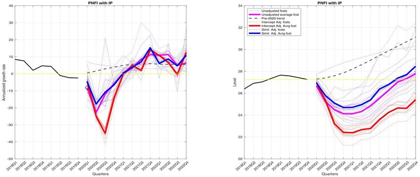
Forecasting in the Absence of Precedent
                                                     Paul Ho∗
                                      Federal Reserve Bank of Richmond†
                                               paul.ho@rich.frb.org

                                                 June 16, 2021

                                                    Abstract

          We survey approaches to macroeconomic forecasting during the COVID-19 pandemic. Due to
          the unprecedented nature of the episode, there was greater dependence on information outside
          the econometric model, captured through either adjustments to the model or additional data.
          The transparency and flexibility of assumptions were especially important for interpreting real-
          time forecasts and updating forecasts as new data were observed. With data available at the
          time of writing, we show how various assumptions were violated and how these systematically
          biased forecasts.

          Key Words: Macroeconomic Forecasting, COVID-19

1        Introduction
The COVID-19 pandemic and the ensuing recession has posed challenges for forecasters. The size
of the fluctuations has been unprecedented, with GDP declining by 9% in 2020Q2, compared to a
maximum quarterly decline of 2% in the Great Recession. In addition, the nature of the shock is
different than past recessions. Economic activity declined due to social distancing measures rather
than, for instance, financial shocks.
        In the presence of large and atypical fluctuations in the economy, the challenge for the econo-
metrician is to construct informative forecasts in the absence of data on the new circumstances of
the pandemic. There is thus a particularly important role for sources of information outside what
one might typically use. The first source is subjective judgement or prior knowledge, typically from
economic theory. Alternatively, one can consider external sources of data. For instance, epidemio-
logical data was of special interest during the pandemic. However, the value of the additional data
depends on knowledge of its joint distribution with the variables of interest, which was not always
easy to determine initially.
    ∗
    I am grateful to Huberto Ennis, Thomas Lubik, and Alex Wolman for comments and suggestions.
    †
    The views expressed herein are those of the author and do not necessarily represent the views of the Federal
Reserve Bank of Richmond or the Federal Reserve System.

                                                         1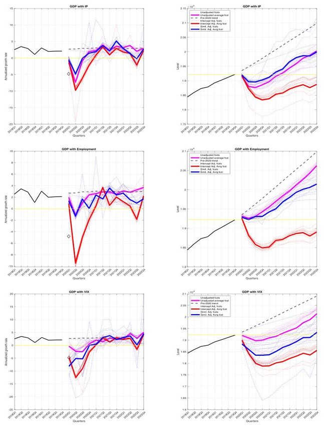
This essay discusses the literature dealing with these challenges during the COVID-19 pandemic.
We highlight assumptions underlying each approach and argue that knowledge of the pandemic
could have been used to interpret and improve these forecasts. We then discuss what the data
through December 2020 tell us about the validity of various assumptions.

2     The Forecasting Problem
2.1   Adapting Economic Models to Unprecedented Times
In adapting our models to allow for the changes in the economy, one needs to acknowledge the
difference in circumstances without going to the extreme of completely ignoring what has been
learnt from past experience. In addition, the particular circumstances can make new data either
unusually informative or misleading, depending on whether one is able to appropriately discern
how the different variables evolve jointly.

Economic Knowledge. The econometrician needs to translate her interpretation of the data’s
large fluctuations into model assumptions. This requires subjective judgement informed by eco-
nomic theory or knowledge outside the model. Is the variation in data explained by large shocks,
new shocks, or a different propagation of shocks? These questions have also been asked in attempts
to account for previous changes in the behavior of macroeconomic data (e.g., Cogley and Sargent
(2005); Sims and Zha (2006); Stock and Watson (2012)).
    Assumptions in the model should be easily communicated. Transparent assumptions allow
the audience to understand forecasts within the context of the model. For example, if the model
assumes an unchanged persistence but it is understood that the current recession is likely to be less
persistent than past experience, then one can take the model forecast as providing an overestimate
of the depth of the recession in the medium run.
    In addition, where possible, assumptions should be imposed probabilistically. For example, even
if one believed that past experience was a good benchmark for how the COVID-19 recession may
play out, one can impose that the model parameters are “probably close”—rather than identical—
to what they were before the pandemic. This allows us to update our parameter estimates as we
observe new data. At the time of writing, we are still in the middle of the pandemic, but have
over a year of data on the evolution of both economic and epidemiological variables. Even with
decades of data, artificially tight prior assumptions can bias model predictions in ways that are
often hard to detect (e.g., Canova and Sala (2009); Giannone et al. (2015); Ho (2020)), a problem
that is exacerbated when data are relatively scarce. Moreover, these assumptions can give a false
sense of precision in forecasts.
    The above features are especially important in the context of the COVID-19 pandemic. Given
disagreement among economists and policymakers, clear communication is crucial for making quan-
titative model forecasts useful beyond the narrow audience that fully agrees with the model as-
sumptions. Since individual econometricians were themselves probably less certain about the new

                                                 2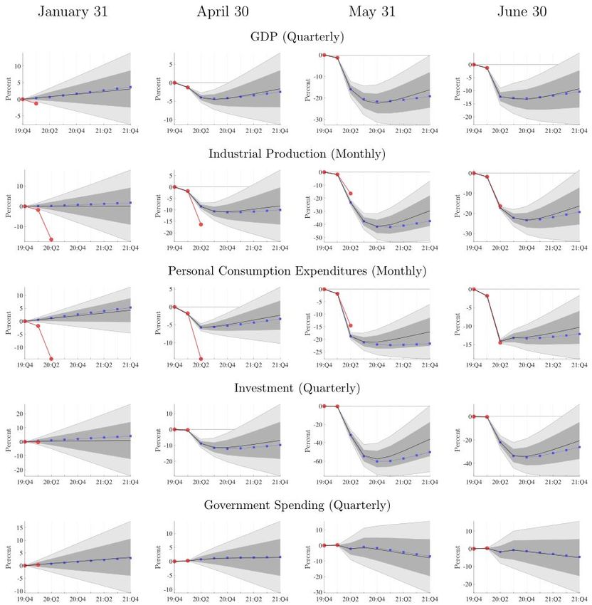
structure of the economy, the probabilistic presentation of assumptions results in forecast error
bands that more accurately reflect the econometrician’s own degree of confidence.

Additional Data. The COVID-19 pandemic was a striking example of when new data sources
became especially useful. The public health dimension of the economic fallout made data on
COVID-19 cases, hospitalizations, and deaths important. In addition, the fast-moving nature of
the crisis brought a new demand for high frequency data to inform economists and policymakers of
the state of the economy before the usual quarterly or even monthly data were published. Beyond
raw data, forecasts of the pandemic were and continue to be of interest (e.g., Ho et al. (2020);
Atkeson et al. (2021); Li and Linton (2021); Liu et al. (2021)).
    The question of how to integrate these data into model forecasts of the economy returns us to
the question of model specification. Assumptions need to be made about the relationship between
the additional data series and the variables one was looking at previously. If these assumptions
are misguided, incorporating the additional data can lead one to misleading conclusions about the
current and future state of the economy.

2.2    Formal Framework
Model. To formally organize our discussion, we consider the vector autoregression (VAR):

                                              Xt = BXt−1 + Cεt ,                                                 (1)

where Xt is a vector of current and lagged macroeconomic variables, and εt ∼ N (0, I) is a vector
of orthogonal shocks normalized to each have variance one. The parameter C determines how a
shock affects the economy on impact, and the parameter B captures how the shock then propagates
through the economy.
    Many forecasting models can be cast as special cases or extensions of this. For example, dynamic
stochastic general equilibrium (DSGE) models and factor models take the form (1) with restrictions
on B and C that arise from either economic or statistical restrictions derived from the respective
models. The time-varying parameter (TVP) VAR (e.g., Primiceri (2005); Lubik and Matthes
(2015)) takes the form (1) but allows B and C to vary over time. More involved methods, especially
from the field of machine learning, have been used for macroeconomic forecasting before and during
the COVID-19 recession (e.g., Coulombe et al. (2021); Huber et al. (2020)). While we do not provide
a detailed description of these methods here, we note that these methods introduce a high degree
of flexibility for the variables Xt to evolve differently during contrasting episodes, which can be
thought of as less parametric approaches to the ideas in Section 3.1.1

    1
      While Coulombe et al. (2021) find that machine learning methods improved forecasting performance over certain
benchmark linear models similar to (1) during the pandemic, it is not clear how these methods compare to parametric
extensions to (1), such as those discussed in Section 3.1. In addition, machine learning methods and nonlinear models
more generally have not been found to have systematic benefits over linear models before the pandemic (see Ferrara
et al. (2015) and Coulombe et al. (2021) for details).

                                                         3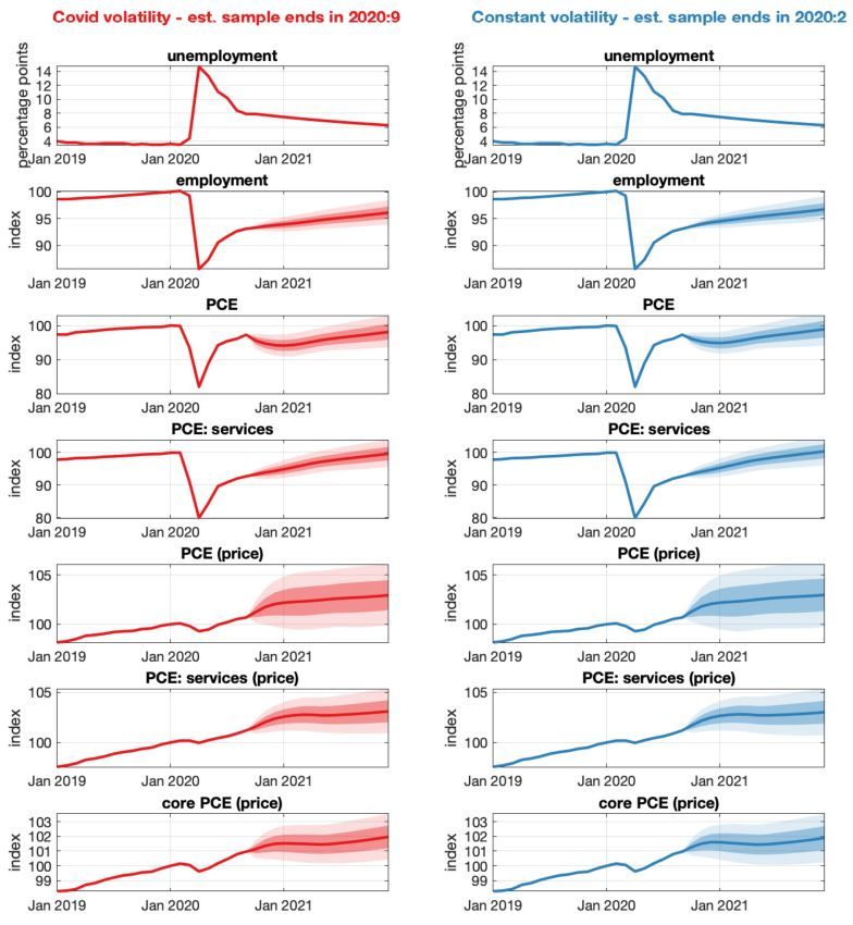
Forecasting.          Suppose all the parameters are known. Then the optimal forecast h periods ahead
is   B h Xt .   One can also condition on a future path for a subset of variables in Xt to derive forecasts
for the rest of Xt .
      Uncertainty in the forecast arises from two sources. First, there is uncertainty about future εt .
The coefficient C directly scales the level of this uncertainty by changing the variance of the errors
Cεt . The coefficient B also impacts uncertainty by influencing the propagation of the shocks εt .
For example, if B implies a very persistent system, then shocks today can have a lasting impact
on macroeconomic outcomes far in the future. As a result, the value of Xt not only depends on
the contemporaneous shock, but is also heavily driven by past shocks, thus increasing the variance.
Second, there is uncertainty about the parameter values for B and C. Even if one knew all future
realizations of εt , the way these impact Xt depends on the parameter values.

Unusual Times. The challenge in uncertain times such as the COVID-19 pandemic, is that the
recent parameters are probably not the ones governing the evolution of the data Xt in the near
future. The large share of temporary layoffs made the initial shock to unemployment less persistent
than in the past (i.e., B was closer to 0). The speed with which social distancing measures were
adopted (both by policy and individual decisions) resulted in larger and more sudden changes in
the economy (i.e., a larger scale of C). The fact that the public health outcomes started playing a
role in business cycle fluctuations that they never had in recent history suggests that there may be
new data series or shocks to consider (i.e., additional relevant series in Xt or new shocks in εt ).
      Typically, one might rely on the data to update our estimates rather than impose assumptions
on how the parameters have changed, potentially through a TVP-VAR that allows parameters
to adjust to the new circumstances. However, the fast-moving nature of the pandemic required
forecasts before sufficient data had been observed to reliably update the parameters. The absence
of data and knowledge that circumstances had changed meant that econometricians have had to
choose how to impose their knowledge of current events on the model forecasts. Moreover, the
uniqueness of the crisis increases uncertainty about what is known before seeing data. For instance,
while there is a rich literature of DSGE models studying typical recessions, quantitative models of
the public health dimension of the COVID-19 crisis have not been widely studied. The literature
has struggled real-time with this—not only is there qualitative disagreement about economic events,
but the high dimensionality of many forecasting models presents challenges to expressing qualitative
views and knowledge quantitatively.2

3         Forecasting Approaches During the COVID-19 Pandemic
We now discuss four attempts to adapt forecasting methods to the COVID-19 pandemic.

      2
    For instance, in the model (1), if Xt contained 12 lags of 6 variables, which is typical with monthly data, B
would have 432 elements to be estimated.

                                                        4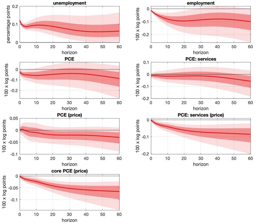
3.1     Adapting the Model
The first two approaches focus on extensions to (1). We discuss how the results may have been
influenced by particular assumptions that each paper makes about how the COVID-19 economy
differs from the pre-pandemic economy.

3.1.1    Increasing Volatility

Lenza and Primiceri (2020) interpret the volatility in the economy during the pandemic as arising
from a sequence of large shocks. In particular, they replace (1) with

                                       Xt = BXt−1 + st Cεt ,                                      (2)

where the additional variable st determines how the variance of the shock varies over time. They as-
sume st = 1 before the pandemic, estimate st for March, April, and May 2020, and assume a gradual
(autoregressive) decay back to one subesquently. The idea of incorporating time-varying volatility
in models is not new (e.g., Engle (1982); Jacquier et al. (2004); Stock and Watson (2016)). In the
forecasting context, Clark (2011) shows that including time-varying volatility improves macroeco-
nomic forecasting performance.
   The change in variance captured in (2) is important for both estimation and forecasting. For
estimation, acknowledging that recent data is subject to a large amount of noise ensures that the
estimates for B and C are not overly impacted by the small number of outliers. Indeed, Lenza
and Primiceri (2020) find that when they estimate (1) instead of (2) using data that includes the
COVID-19 periods, the model produces unreasonable forecasts with explosive responses to shocks
that can predict that the recession continually deepen without any end. Huber et al. (2020) provide
an alternative approach to dealing with outliers using a nonparametric model. Their approach
recognizes the increased uncertainty when the data look different than in the past, as was the case
in 2020Q2 and 2020Q3. While Lenza and Primiceri (2020) attribute the difference to a large shocks,
Huber et al. (2020) allow for a change in parameters.
   For forecasting, since a large part of forecast uncertainty arises from the possibility of future
disturbances, acknowledging the increased variance of shocks captures the increased uncertainty in
forecasts. Carriero et al. (2021a) show that assumptions about the time-varying volatility st matter
for forecasts. They distinguish between allowing st to fluctuate gradually (as a random walk both
before and after the COVID-19 pandemic) and allowing for occasional one-off jumps in st . Because
the March and April 2020 data were such huge outliers, allowing for occasional one-off jumps in the
shock variances tightens forecast error bands, arguably making them more reasonable by allowing
volatility to quickly return to closer to historical levels after the initial sharp adjustments to the
pandemic. In related work, Carriero et al. (2021b) estimate a time-varying volatility VAR using
data through June 2020 and find a substantial role for such one-off increases in volatility in a
number of variables, including employment and industrial production.
   There are two attractive features of the Lenza and Primiceri (2020) approach. First, the as-

                                                  5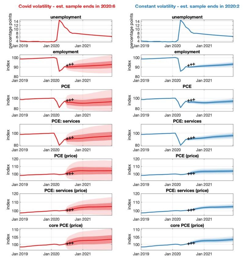
sumptions are transparent to communicate. Even if one does not believe the exact model, the
forecasts can be informative if one has a clear idea of the direction in which they are biased.
Second, estimation is a straightforward application of generalized least squares.
   There are two implicit assumptions that are potentially problematic:

  1. Since B remains unchanged, the effect of a one time shock εt propagates through the economy
        the same way before and during the pandemic.

  2. The variance of all shocks increases proportionally.

In other words, (2) treats the pandemic as merely a period with unusually high volatility even
though there was an understanding early on in the pandemic that the COVID-19 recession would
differ from previous recessions in terms of job losses, revenue losses, and consumer behavior. As
a result, both the propagation of and the relative variance of shocks likely differed from the pre-
pandemic data. These assumptions are dropped, for instance, in the TVP-VAR of Primiceri (2005)
or Lubik and Matthes (2015).
   Lenza and Primiceri (2020) present forecasts conditional on actual unemployment data through
September 2020 and Blue Chip consensus forecasts for unemployment in subsequent months. They
compare the forecasts from (2) to an estimation without accounting for the change in variance (using
only pre-pandemic data for the estimation of the parameters). The conditional forecasts from June
2020, shown in Figure 1, show that the inclusion of the time-varying variance substantially widens
the forecast error bands, as the model predicts a future sequence of large shocks (i.e., large future
st ). In contrast, when a fixed variance is assumed, the forecast error bands are much narrower,
with realized data falling outside or on the edge of the 95% credible region. Figure 2 shows that
the time-varying variance no longer has a significant effect on the size of the error bands when the
forecast is made using data through September 2020. By this time, the estimated variance is closer
to normal and parameter uncertainty is the main source of forecast uncertainty.
   While the approach of Lenza and Primiceri (2020) helps account for uncertainty, it leaves the
point forecasts relatively unchanged, reflecting a relatively unchanged coefficient B. Even though
data from the COVID-19 period can potentially alter the estimate of B, the estimation places very
low weight on these data due to their large variance, captured by st . For the conditional forecasts
in Figures 1 and 2, this turns out to be a reasonable assumption, as the distribution of employment,
consumption, and prices conditional on unemployment did not change too much.3 We will show
later that this was not true for other variables. In addition, the assumption of a constant B would
have likely resulted in misleading unconditional forecasts. The highly persistent response of the
economy to an unemployment shock, shown in Figure 3, suggests that the model would not have
predicted the relatively rapid decline in unemployment shortly after the start of the pandemic. The
response is consistent with the historical behavior of employment but not necessarily the specific
circumstances of the COVID-19 recession.

   3
       The Blue Chip forecasts overpredicted unemployment, lowering forecasts for employment and consumption.

                                                        6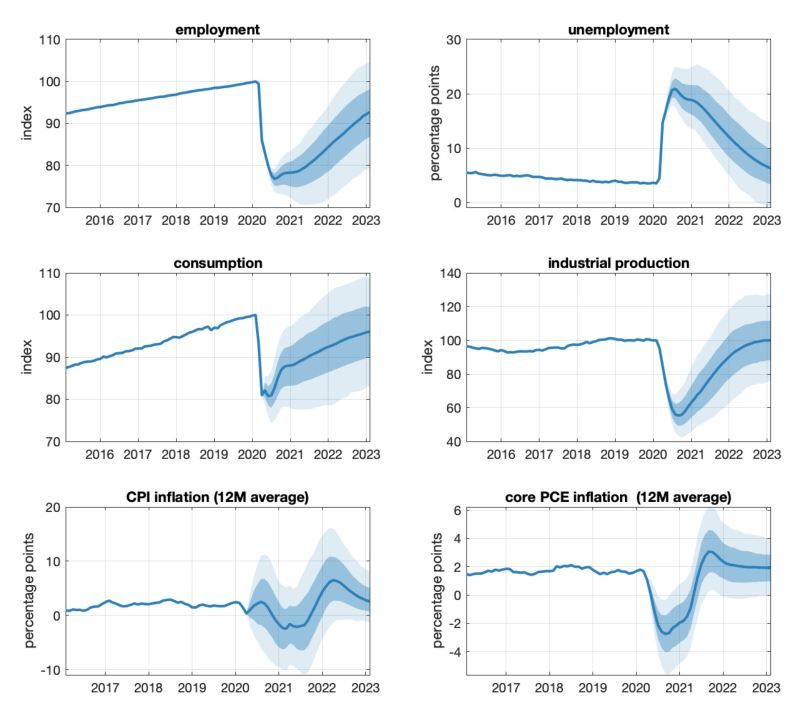
Figure 1: Figure 3 from Lenza and Primiceri (2020). Forecasts as of June 2020 conditional on path
for unemployment (actual realizations until September 2020, Blue Chip consensus forecasts subse-
quently), 68% and 95% bands. Crosses are data realizations. Left panel: Estimation with change
in volatility using data through June 2020; Right panel: Estimation with constant volatility using
data through February 2020.

                                                7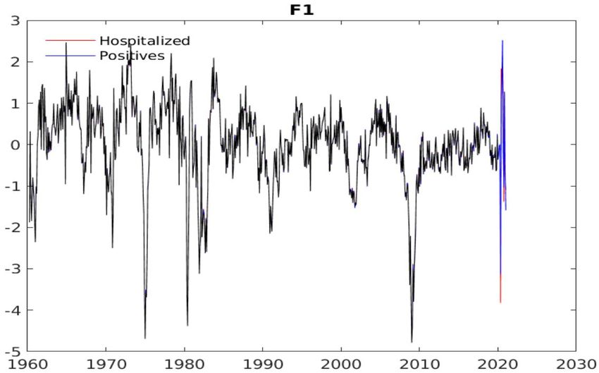
Figure 2: Figure 4 from Lenza and Primiceri (2020). Forecasts as of September 2020 conditional on
path for unemployment (actual realizations until September 2020, Blue Chip consensus forecasts
subsequently), 68% and 95% bands. Crosses are data realizations. Left panel: Estimation with
change in volatility using data through September 2020; Right panel: Estimation with constant
volatility using data through February 2020.

                                               8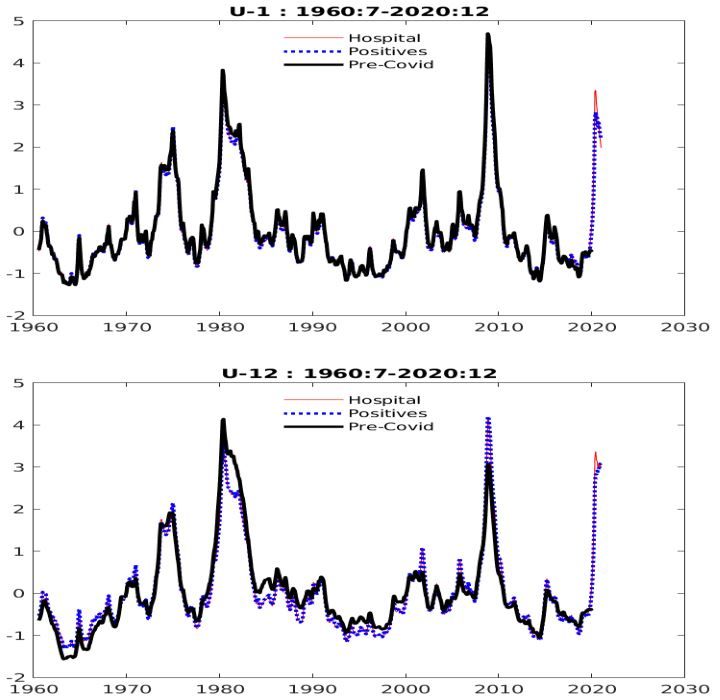
Figure 3: Figure 2 from Lenza and Primiceri (2020). Impulse response to a one standard deviation
unemployment shock, 68% and 95% bands.

3.1.2   Introducing a New Shock

Primiceri and Tambalotti (2020) provide a framework that acknowledges that the COVID-19 shock
is different than previous shocks, weakening the assumptions in Lenza and Primiceri (2020). We
present a simplified version of their approach using the VAR model (1). Noting that (1) can be
                    P∞       s Cε
rewritten as Xt =    s=0 B       t−s ,   with the data being explained by an infinite history of shocks,
Primiceri and Tambalotti (2020) consider a version of the model:
                                          ∞
                                          X                 ∞
                                                            X
                                                 s
                                  Xt =          B Cεt−s +         Gs H ◦ vt−s ,                      (3)
                                          s=0               s=0

where vt is the COVID-19 shock that takes the value zero before March 2020 and ◦ denotes element-

                                                      9
wise multiplication.4
At its core, the above procedure is forecasting conditional on an unobserved variable vt . The
path of shocks is hypothetical but can in principle be derived from external data such as mobility
measures or case numbers, as will be illustrated in Section 4. How successful and reasonable the
forecasts are depend on the assumptions made about the path of the COVID-19 shock and its
propagation through the economy. Primiceri and Tambalotti (2020) make three assumptions:
1. The variable vt accounts for all unexpected variation of Xt in March and April 2020.
2. G = B, i.e., the way the shock propagates through the economy remains unchanged, similar
to the assumption in Lenza and Primiceri (2020) that B remains unchanged.
3. The variable vt is generated by a sequence of typical business cycle shocks, as defined based
on a fully-specified DSGE model from Justiniano et al. (2010).
Assumption 1 is a reasonable approximation ex ante because COVID-19 has overshadowed all other
typical variation in the economy. It is the typical assumption made in event studies.
Assumptions 2 and 3 are more controversial. Both assumptions treat the COVID-19 shock as
typical even though the nature of the COVID-19 shock to the economy is vastly different from
any recent experience. Moreover, the rigidity of the assumptions imply that incoming data have
limited capacity to revise model estimates. Nevertheless, completely discarding past experience
would result in overly uninformative forecasts. Even though the shock is unusual, the structure of
the economy does not completely change overnight.
Forecasters should acknowledge the unprecedented situation while allowing the model to be
informed by data. For the propagation of shocks, we consider the pre-pandemic value of B is a
good benchmark but expect the economy to recover more rapidly than in previous recessions. This
should be imposed probabilistically, replacing Assumption 2, so that we do not force our beliefs
on the data but instead allow the forecasts to combine our beliefs with the available data. For
the evolution of the shock, epidemiological model forecasts can replace Assumption 3 by providing
informed predictions about the future path of the pandemic and uncertainty about that path.5
Through the lens of a TVP-VAR, the new shock in Primiceri and Tambalotti (2020) can be
captured through a change in parameters. Starting with an initial belief about the parameter
values that is centered at the pre-pandemic estimates, the TVP-VAR allows the data to inform the
estimates of a potentially new set of parameters. The model has the flexibility to allow for changes
in comovements, persistence, and variances.
Figure 4 shows that Primiceri and Tambalotti (2020) forecast a more persistent decline in
economic activity than occured. Their forecast conditions on vt being close to zero from around
January 2021, which has turned out to be an overly optimistic prediction. Nevertheless, even the
4
P∞
More precisely, Primiceri and Tambalotti (2020) take vt = r u , where ut is a scalar that takes value
s=o s t−s
one in March 2020 and zero for all other months.
5
For example, Meza (2020) implements the Primiceri and Tambalotti (2020) methodology for Mexican data,
conditioning forecasts on the path of the pandemic predicted by a simple epidemiological model.
10Figure 4: Figure 2 from Primiceri and Tambalotti (2020). Forecasts from April 2020 under baseline
scenario for vt , 68% and 95% bands.
95% forecast error bands do not include the rapid rebound in unemployment and consumption that
we have seen since the early weeks of the pandemic. Allowing for the widely discussed possibility
of the COVID-19 shock having a more transitory effect than previous recessions (i.e., G closer to 0
than B) would have widened the error bands, providing a quantitative forecast that more accurately
reflected the debate at the time of the forecast and one that is ex post more accurate.
3.2 Additional Information in the Data
Whereas the approaches above keep the same variables but modify the model, the next two ap-
proaches seek to utilize recent and past data to improve forecasts. We emphasize that the ability to
leverage information in the data depends on valid assumptions about the comovement of variables.
113.2.1 Learning from Higher Frequency Data
Given how rapidly the effects of the pandemic were felt and how swiftly policymakers have had
to respond, it has been crucial to incorporate high frequency data to ensure that we are using all
available information for our forecasts. To that end, several papers have used mixed-frequency
(MF) models for forecasting. In the context of (1), these papers allow for the econometrician to
only observe Xt or averages of Xt in particular periods, which provides the possibility of incorpo-
rating data of different frequencies in Xt (e.g., monthly industrial production and quarterly GDP).
Intuitively, the joint behavior of Xt allows us to infer the values of unobserved elements of Xt .
During the pandemic, it was reasonable to expect that these joint distributions might have evolved
(i.e., B and C in equation (1) changed). Without accounting for these changes, one may draw
misleading conclusions from the high frequency data.
An illustration of the role of high frequency data in informing forecasts is provided by Schorfheide
and Song (2020), who present real-time macroeconomic forecasts during the pandemic using a
relatively standard model from Schorfheide and Song (2015). They include three quarterly series
(GDP, investment, and government expenditures) and eight monthly series (unemployment rate,
hours worked, Consumer Price Index, industrial production, Personal Consumption Expenditure,
Federal Funds Rate, 10-year Treasury Bond Yield, and S&P 500 Index). For the results we will
discuss, the underlying parameters B and C are estimated using data available on January 31,
2020, and forecasts are updated purely from new information about the realized path of the data
rather than changes in parameter values.6
We find mixed success comparing the realizations of the 2020Q2 data to what is forecast by the
model using data available on June 30, 2020. By this time, the quarter had come to an end, but
the GDP numbers had not yet been announced. GDP fell to 10% below the 2019Q4 level, close to
the Schorfheide and Song (2020) median forecast of 12% and within the 60% predictive bands. On
the other hand, 2020Q2 investment fell 9% relative to 2019Q4, substantially less than the June 30
median forecast of 22% and even the 95% quantile of 16%. Note that the quantiles already capture
the inherent relative volatility of the respective series, with the error bands for investment double
the width of those for GDP.
The fact that the GDP nowcast (i.e., the forecast of current quarter GDP before it has been
reported) performs so well relative to the investment nowcast suggests a change in the relationship
between the monthly and quarterly variables. This is a similar issue to that raised in our discussion
of Lenza and Primiceri (2020) and Primiceri and Tambalotti (2020)—there were features of the
data during the pandemic that we might have expected ex ante to have changed, but the model
forecasts did not take these into account. Economic theory suggests that investment should fall
less for more transitory shocks. Given the ex ante likelihood that the COVID-19 recession would
be more short-lived than past recessions, one might have expected that the response of investment
6
When the data after January 2020 were used for estimation, Schorfheide and Song (2020) run into the challenge
highlighted by Lenza and Primiceri (2020), as the pandemic era outliers result in unreasonable parameter estimates,
leading to poor forecasts.
12Figure 5: Figure 3 from Schorfheide and Song (2020). Forecasts from January 31, April 30, May
31, and June 30, 2020, realized data (solid red) and median forecast (solid black) with 60% and
90% bands. Solid blue line represents point forecasts obtained by fixing the federal funds rate at 5
basis points. All variables are plotted relative to their 2019Q4 levels.
13relative to the movement in the monthly series would be muted.
The forecasts updated dramatically as monthly data is observed during the initial decline of
economic activity between April to June. On April 30, May 31, and June 30, Schorfheide and Song
(2020) forecast 2020Q2 GDP of 4%, 15%, and 12% below the 2019Q4 level, respectively. These
updates are large not only relative to past data, but also relative to the error bands of the forecasts.
Moreover, none of these updates are arising from changes in the underlying parameters. To justify
such large updates, one needs to interpret the shocks in May and June as being extremely low
probability events given the April 30 data. Given the uniqueness of the period, the plausibility of
such an interpretation depends on subjective judgement.
Koop et al. (2021) study a similar model and ask how allowing for different forms of time-varying
volatility, in the spirit of Lenza and Primiceri (2020), affects nowcasts for GDP. While the point
nowcasts do not differ substantially, time-varying volatility leads to larger nowcast error bands.
In addition, imposing time-invariant variances leads to a more rapid update of the nowcasts as
high frequency data are observed. Given the short sample, evaluating which of these nowcasts are
preferred requires subjective judgement.
An alternative to increasing the time series dimension through high frequency data is to focus on
the cross section studying panel data. For example, Aaronson et al. (2020) and Larson and Sinclair
(2021) find some success using the panel of U.S. states (together with data on Google Trends and
state of emergenecy declarations) to improve nowcasts of unemployment insurance (UI) claims.
3.2.2 Learning from Past Crises
One response to the shortcomings in Schorfheide and Song (2020) is to ask if there are historical
episodes that can suggest where our current estimated model might make errors. To that end,
Foroni et al. (2020) adjust forecasts from various MF models using information from the Great
Recession. The class of models used can be viewed as minor modifications of (1).7 In what follows,
we reference our benchmark VAR model (1) instead of the actual models in Foroni et al. (2020) in
order to economize on notation and simplify the exposition.
First, they compute similarity adjusted forecasts in which they increase the weight on observa-
tions from the Great Recession. The reweighting captures the idea that the COVID-19 economy
is more similar to the Great Recession than the average time period. In the notation of (1), this
changes the estimates of B and C to be closer to the values that best fit the Great Recession period.
Second, they produce intercept adjusted forecasts by correcting forecasts based on forecast
errors made during the Great Recession. The correction accounts for systematic bias that may
occur during recessions. Formally, rather than take B h Xt as the h-period-ahead forecast, they use
B h Xt + ut∗ , where ut∗ is the forecast error from the corresponding period in the Great Recession.
Foroni et al. (2020) generate forecasts using data available in April 2020, which includes monthly
7
PK PL PM
More precisely, Foroni et al. (2020) consider yt+h = β y
k=0 k t−k
+ l=0 δl xt−l + m=0 γm ut−m , where yt is
the variable of interest, xt contains additional predictors, and ut captures the forecast error. The variety of models
involve different assumptions on βk and δl as well as different methods of estimation.
14observations for the beginning of the pandemic but only includes quarterly data through 2019Q4.
They focus on quarterly forecasts of GDP and investment but include monthly data on industrial
production, employment, or the VIX as additional predictors. They consider a range of models
that differ based on the number of lags included and assumptions about the parameters.
The forecast error correction substantially changes the forecasts but the reweighting of obser-
vations does not.8 However, with the benefit of hindsight, we see that the model substantially
underpredicts the initial decline in GDP but overpredicts the persistence of the decline in GDP
growth, with forecast annualized declines of approximately 10% and 5% in 2020Q2 and 2020Q3,
respectively, in contrast to the 33% decline and 38% increase in the data. Foroni et al. (2020)
forecast a decline in investment that had a trough level close to the data but overpredict the persis-
tence of this decline. Their forecasts are roughly in line with the Schorfheide and Song (2020) April
2020 forecasts. Like Schorfheide and Song (2020), Foroni et al. (2020) overpredict the decline of
investment relative to GDP as they fail to acknowledge the differences in the COVID-19 recession.
Instead of using the Great Recession, Ludvigson et al. (2021) use data on past natural disasters to
predict the economic effects of the COVID-19 pandemic. They also find mixed success depending
on the variable, performing relatively well for industrial production but poorly for initial claims
and service sector employment. Similarly, Aaronson et al. (2020) use the comovement between UI
claims and Google Trends during recent hurricanes in the U.S. to forecast UI claims during the
pandemic.
The forecast errors in Foroni et al. (2020) are unsurprising ex post but might also be expected
ex ante. The COVID-19 recession has been larger, more rapid, and less persistent than the Great
Recession. These differences were considered distinct and even likely possibilities in March. In
principle, one could have used the results from Foroni et al. (2020) as bounds for forecasts, assuming
a belief about how the COVID-19 recession would evolve relative to the Great Recession. For
conditional forecasting, Foroni et al. (2020) also provide a way to generate plausible bounds on the
paths of variables that we choose to condition our forecasts on. More generally, even though we
may perceive clear differences between the current situation and previous recessions, knowing the
direction of these differences can allow us to productively incorporate past experience to refine our
forecasts.
4 Looking Back at What Changed
While the literature above focused on forecasting the economy real time during the pandemic, it is
useful to look back on data that we now have, both economic and epidemiological, to understand
what assumptions turned out to be valid. Ng (2021) provides one perspective on this question.
The paper incorporates COVID-19 epidemiological data and provides insight into two questions:
1. Controlling for COVID-19 data, did the structure of the economy change?
8
These results are consistent with Stock and Watson (2012) who, using a different model, find that the evolution
of the macroeconomic variables during the Great Recession was due to large shocks rather than structural changes
in the economy.
15Figure 6: Figure 6 from Foroni et al. (2020). Forecasts for GDP, unadjusted (magenta), intercept
adjusted (red), and similarity adjusted (blue). Solid lines average across models, dotted lines
indicate individual models.
16Figure 7: Figure 10 from Foroni et al. (2020). Forecasts for investment, unadjusted (magenta),
intercept adjusted (red), and similarity adjusted (blue). Solid lines average across models, dotted
lines indicate individual models.
2. Controlling for COVID-19 data, how volatile were the data?
The paper is also an example of how epidemiological data can be easily incorporated into our
econometric models. While this may have been harder to accomplish early in the pandemic, we
now have sufficient data to inform our estimates.
For the question on the structure of the economy, Ng (2021) estimates the factor model:
Xt = HFt + αzt + ut , (4)
where Xt is a large panel of over one hundred macroeconomic and financial indicators, Ft is a small
number of unobserved factors that account for the comovement in Xt , and zt is a moving average
of the growth in either COVID-19 cases or COVID-19 hospitalizations. The COVID-19 variable zt
is set to zero before the pandemic. She estimates (4) using data through February 2020, and then
data through December 2020. If zt fully captures all the changes in the comovement of the different
variables, then the coefficients H and estimated factors Fbt will not be substantially affected by the
inclusion of 2020 data. As we have discussed in Section 3, the stability of relationship between
macroeconomic variables is a critical issue for econometricians to confront.
Ng (2021) finds that the factors do not change substantially. In particular, Figure 8 shows
three different estimates for the first macroeconomic factor—one using data through February 2020
and two using data through December 2020 with COVID-19 hospitalization or case data. The
three lines overlap almost perfectly. Ng (2021) reports that for the other factors (not plotted), the
estimates with data through December 2020 have a correlation of at least 0.65. The correlation
is close to one for about half the factors. These high correlations suggest that changes in the
comovement in the economy during the pandemic can mostly be explained by COVID-19 data. It
is somewhat surprising that simply incorporating COVID-19 data can reverse the result in Lenza
17Figure 8: Figure 2 from Ng (2021). First macroeconomic factor estimated using data through
February 2020 (black) and using data through December 2020 with hospitalization (red) or case
(blue) data.
and Primiceri (2020) that the pandemic era macreconomic data can severely impact parameter
estimates. It suggests, for instance, that the COVID-19 variable zt can capture much of the change
in the fluctuations of GDP and investment relative to other variables in the economy, which we
highlighted in our discussion of Schorfheide and Song (2020) and Foroni et al. (2020).
On the question of volatility, Ng (2021) estimates the following model:
(h) (h)
xi,t+h = βi Fbt + γi,h Zt + vi,t+h , (5)
where xi,t+h is one of the data series, Fbt are the factors estimated from (4), Zt are the moving
(h)
averages of the growth in COVID-19 cases and hospitalizations, and vi,t+h are h-period-ahead
forecast errors. For each period t and a given horizon h, she computes an “uncertainty index” based
on Jurado et al. (2015) by averaging the variances of the vi,t+h across the various series.
This uncertainty index provides a measure of the volatility of the shocks (both idiosyncratic
and common) in the economy. Recall that in Section 3, the change in volatility was the only change
considered by Lenza and Primiceri (2020). On the other hand, Primiceri and Tambalotti (2020)
assumed that the traditional macroeconomic shocks were negligible in March and April, but at
historical levels of volatility subsequently. The estimated coefficients γi,h in equation (5) allow us
to test for evidence of a new shock. Assuming Zt captures the COVID-19 shock, the uncertainty
index is a measure of whether volatility was particularly high compared to historical episodes.
Figure 9 shows that the uncertainty index reaches approximately the level of the 1973-74,
1981-82, and 2007-09 periods. In other words, while the level of volatility was high by historical
standards, it was not unprecedented. It is important, however, to note that the uncertainty index
18Figure 9: Figure 4 from Ng (2021). Uncertainty index estimated using data through February 2020
(black) and using data through December 2020 with hospitalization (red) or case (blue) data. Top
panel: one-month-ahead forecasts (i.e., h = 1); Bottom panel: twelve-month-ahead forecasts
(i.e., h = 12).
is designed to capture shock volatility rather than parameter uncertainty since the parameters are
estimated using the full data sample through December 2020. In particular, at the early stages of
the pandemic, we did not have the data needed to obtain precise estimates of γi,h in equation (5)
or α in equation (4). As a result, if we were estimating the same models real time, there would
be a substantially larger amount of parameter uncertainty to deal with, which should imply larger
error bands in one’s real-time forecasts.
Ng (2021) finds that the coefficients γi,h on the COVID-19 data in equation (5) are important
for predicting xi,t+h . The relevance of the COVID-19 data emphasizes the new significance of
epidemiological data in determining macroeconomic fluctuations, even after accounting for the
factors Fbt . This supports the interpretation by Primiceri and Tambalotti (2020) of COVID-19
introducing a new shock to the economy. The importance is further emphasized by contrasting the
results in Ng (2021) with those in Carriero et al. (2021b), who estimate a time-varying volatility VAR
without including COVID-19 data and find historic increases in their measures of volatility. For
instance, in their benchmark model, Carriero et al. (2021b) report peak macroeconomic uncertainty
level of 7.6, about three times the Great Recession peak.
19An important caveat in the results is that the data Xt used by Ng (2021) are cleaned to fit
the factor structure. First, the data are demeaned, with different means for data before and after
March 2020. Second, a dummy is included for March 2020 that absorbs the initial large variation.
The results should be interpreted as capturing the variation around these two different means after
ignoring the initial large impact rather than the full extent of fluctuations.
5 Conclusion
When forecasting in the absence of precedent, one needs to tap on information outside one’s typ-
ical models to construct informative forecasts. We have illustrated approaches of using external
knowledge or new data sources that the literature has discussed. As we look back on the successes
and failures of the various forecasts, we find that a greater acknowledgement of the particular
circumstances of the pandemic could have led to more accurate forecasts. As an econometrician,
one has to balance feasibility, transparency, and sophistication in one’s models. As a consumer of
these forecasts, one has to then interpret each forecast in the context of the assumptions. However,
until the assumptions have been modeled probabilistically, it is difficult to know what quantitative
adjustment one should make to one’s forecasts to account for changes in the economy.
With hindsight, one can analyze which assumptions turned out to be valid. However, this is
not straightforward even after the event. For instance, while Sims and Zha (2006) argue that the
Great Moderation is best explained by a reduction in volatility, Primiceri (2006) and Sargent et al.
(2006) argue that the decline in inflation should be explained by policymakers learning and adapting
policy. A similar debate is found in Stock and Watson (2012) and the accompanying discussion.
The difficulty in establishing what changed in the economy ex post emphasizes the substantial role
for parameter uncertainty in the middle of an unprecedented episode.
While this essay has used the COVID-19 pandemic as a case study, the themes apply to other
rare events and even normal times. Assumptions often mask uncertainty and bias forecasts. Addi-
tional data is informative insofar as it is appropriately modeled. Models should have the flexibility
for parameter estimates to adjust probabilistically to incoming data, and forecasters should trans-
parently communicate limitations in this learning process.
20References
Aaronson, D., S. A. Brave, R. A. Butters, D. W. Sacks, and B. Seo (2020). Using the Eye of the
Storm to Predict the Wave of Covid-19 UI Claims. Covid Economics 9, 59.
Atkeson, A. G., K. Kopecky, and T. Zha (2021). Behavior and the Transmission of COVID-19.
AEA Papers and Proceedings 111, 356–60.
Canova, F. and L. Sala (2009). Back to Square One: Identification Issues in DSGE Models. Journal
of Monetary Economics 56 (4), 431–449.
Carriero, A., T. E. Clark, M. G. Marcellino, and E. Mertens (2021a). Addressing COVID-19
Outliers in BVARs with Stochastic Volatility. Federal Reserve Bank of Cleveland Working Paper
21-02.
Carriero, A., T. E. Clark, M. G. Marcellino, and E. Mertens (2021b). Measuring Uncertainty and
Its Effects in the COVID-19 Era. Centre for Economic Policy Research Working Paper DP15965.
Clark, T. E. (2011). Real-Time Density Forecasts From Bayesian Vector Autoregressions With
Stochastic Volatility. Journal of Business & Economic Statistics 29 (3), 327–341.
Cogley, T. and T. J. Sargent (2005). Drifts and Volatilities: Monetary Policies and Outcomes in
the Post WWII U.S. Review of Economic Dynamics 8 (2), 262–302.
Coulombe, P. G., M. Marcellino, and D. Stevanovic (2021). Can Machine Learning Catch the
COVID-19 Recession? Centre for Economic Policy Research Working Paper DP15867.
Engle, R. F. (1982). Autoregressive Conditional Heteroscedasticity with Estimates of the Variance
of United Kingdom Inflation. Econometrica, 987–1007.
Ferrara, L., M. Marcellino, and M. Mogliani (2015). Macroeconomic Forecasting During the Great
Recession: The Return of Non-Linearity? International Journal of Forecasting 31 (3), 664–679.
Foroni, C., M. G. Marcellino, and D. Stevanović (2020). Forecasting the COVID-19 Recession and
Recovery: Lessons from the Financial Crisis. International Journal of Forecasting, Forthcoming.
Giannone, D., M. Lenza, and G. E. Primiceri (2015). Prior Selection for Vector Autoregressions.
Review of Economics and Statistics 97 (2), 436–451.
Ho, P. (2020). Global Robust Bayesian Analysis in Large Models. Federal Reserve Bank of Rich-
mond Working Paper 20-07.
Ho, P., T. A. Lubik, and C. Matthes (2020). How To Go Viral: A COVID-19 Model with Endoge-
nously Time-Varying Parameters. Journal of Econometrics, Forthcoming.
Huber, F., G. Koop, L. Onorante, M. Pfarrhofer, and J. Schreiner (2020). Nowcasting in a Pandemic
Using Non-Parametric Mixed Frequency VARs. Journal of Econometrics, Forthcoming.
21Jacquier, E., N. G. Polson, and P. E. Rossi (2004). Bayesian Analysis of Stochastic Volatility
Models with Fat-Tails and Correlated Errors. Journal of Econometrics 122 (1), 185–212.
Jurado, K., S. C. Ludvigson, and S. Ng (2015). Measuring Uncertainty. American Economic
Review 105 (3), 1177–1216.
Justiniano, A., G. E. Primiceri, and A. Tambalotti (2010). Investment Shocks and Business Cycles.
Journal of Monetary Economics 57 (2), 132–145.
Koop, G., S. McIntyre, J. Mitchell, and A. Poon (2021). Nowcasting ‘True’ Monthly U.S. GDP
During the Pandemic. Centre for Applied Macroeconomic Analysis Working Paper 14/2021.
Larson, W. D. and T. M. Sinclair (2021). Nowcasting Unemployment Insurance Claims in the Time
of COVID-19. International Journal of Forecasting, Forthcoming.
Lenza, M. and G. E. Primiceri (2020). How to Estimate a VAR After March 2020. Working Paper.
Li, S. and O. Linton (2021). When Will the COVID-19 Pandemic Peak? Journal of Economet-
rics 220 (1), 130–157.
Liu, L., H. R. Moon, and F. Schorfheide (2021). Panel Forecasts of Country-Level Covid-19 Infec-
tions. Journal of Econometrics 220 (1), 2–22.
Lubik, T. A. and C. Matthes (2015). Time-Varying Parameter Vector Autoregressions: Specifi-
cation, Estimation, and an Application. Federal Reserve Bank of Richmond Economic Quar-
terly (4Q), 323–352.
Ludvigson, S. C., S. Ma, and S. Ng (2021). COVID-19 and the Costs of Deadly Disasters. AEA
Papers and Proceedings 111, 366–70.
Meza, F. (2020). Forecasting the Impact of the COVID-19 Shock on the Mexican Economy. Working
Paper.
Ng, S. (2021). COVID-19 and Estimation of Macroeconomic Factors. Working Paper.
Primiceri, G. E. (2005). Time Varying Structural Vector Autoregressions and Monetary Policy.
Review of Economic Studies 72 (3), 821–852.
Primiceri, G. E. (2006). Why Inflation Rose and Fell: Policy-Makers’ Beliefs and U.S. Postwar
Stabilization Policy. Quarterly Journal of Economics 121 (3), 867–901.
Primiceri, G. E. and A. Tambalotti (2020). Macroeconomic Forecasting in the Time of COVID-19.
Working Paper.
Sargent, T., N. Williams, and T. Zha (2006). Shocks and Government Beliefs: The Rise and Fall
of American Inflation. American Economic Review 96 (4), 1193–1224.
22Schorfheide, F. and D. Song (2015). Real-Time Forecasting with a Mixed-Frequency VAR. Journal
of Business & Economic Statistics 33 (3), 366–380.
Schorfheide, F. and D. Song (2020). Real-Time Forecasting with a (Standard) Mixed-Frequency
VAR During a Pandemic. Federal Reserve Bank of Philadelphia Working Paper 20-26.
Sims, C. A. and T. Zha (2006). Were There Regime Switches in U.S. Monetary Policy? American
Economic Review 96 (1), 54–81.
Stock, J. H. and M. W. Watson (2012). Disentangling the Channels of the 2007-09 Recession.
Brookings Papers on Economic Activity (1), 81–135.
Stock, J. H. and M. W. Watson (2016). Core Inflation and Trend Inflation. Review of Economics
and Statistics 98 (4), 770–784.
23You can also read