Forward to the Past: Short-term effects of the rent freeze in Berlin - Department of Economics Working Paper No. 308 Anja M. Hahn Konstantin A ...
←
→
Page content transcription
If your browser does not render page correctly, please read the page content below
Department of Economics
Working Paper No. 308

Forward to the Past: Short-term
effects of the rent freeze in
Berlin

Anja M. Hahn
Konstantin A. Kholodilin
Sofie R. Waltl

December 2020

Forward to the Past: Short-Term Effects of the Rent Freeze in
                              Berlin
                Anja M. Hahna , Konstantin A. Kholodilinb,c , Sofie R. Waltla,d
                         a
                           Vienna University of Economics and Business, Austria
                                          b
                                            DIW Berlin, Germany
                                    c
                                      NRU HSE St. Petersburg, Russia
                      d
                        Luxembourg Institute of Socio-Economic Research, Luxembourg

Abstract

In 2020, Berlin enacted a rigorous rent-control policy: the “Mietendeckel” (rent freeze), aim-
ing to stop rapidly growing rental prices. We evaluate this newly enacted but old-fashionably
designed policy by analyzing its immediate supply-side effects. Using a rich pool of rent ad-
vertisements reporting asking rents and comprehensive dwelling characteristics, we perform
hedonic-style Difference-in-Difference analyses comparing trajectories of dwellings inside and
outside the policy’s scope. We find no immediate effect upon announcement of the policy. Yet
advertised rents drop significantly upon the policy’s enactment. Additionally, we document a
substitution effect affecting the rental markets of Berlin’s (unregulated) satellite city Potsdam
and adjacent smaller municipalities. On top, the supplemental quantity analyses reveal a stark
reduction of the number of advertised rental units hampering a successful housing search for
newcomers, (young) first-time renters and tenants aiming for a different housing opportunity.
Keywords: First-Generation Rent Control; Rent Freeze; Urban Policy; Rent Price; Supply
Disruptions; Berlin
JEL classification: C14; C43; O18.

Acknowledgments and Disclaimer: Our findings were covered by the Austrian newspaper “Die
Presse” on 29 November 2020.
This article uses data kindly provided by Empirica Systeme (www.empirica-systeme.de). The re-
sults presented may not correspond to those of the data providers. Any remaining errors are ours.
Corresponding author: kkholodilin@diw.de.
1. Introduction
Standard economic theory generally argues against rent control due to disturbances in the
tenant-unit matching process (Glaeser and Luttmer, 2003). Despite these economic arguments,
such policies are ever and again taken advantage of by politicians as soon as housing markets
become tight. After decades of relatively moderate rent control, in 2010s housing rents started
to rise rapidly and Germany began to expand rent control again. In 2015, the so-called “rent
brake” (in German: Mietpreisbremse) was introduced (Mense et al., 2018; Thomschke, 2019)
and similar policies were adopted internationally, namely in 2018 in France and in 2020 in
Catalonia.
In February 2020, a more radical additional rent control policy came into force in Germany’s
capital Berlin: the rent freeze (in German: Mietendeckel ), a policy responding to soaring rents1
by basically switching off fundamental market economy mechanisms.
Unlike typical policies implemented from the 1970s onward, this latest one appears old-
fashioned: The rent freeze caps the absolute demanded rent price and may hence be labeled as
a first-generation rent control policy in contrast to nowadays’ common policies tailored around
limiting rent increases (second-generation rent control). The rent freeze is also exceptional in
another domain: Ever since 1919, when rent regulations were introduced in Baden and Prussia,
it is the first case of a rent control policy in Germany imposed by a state rather than by the
federal government.
While the return from rent stabilization to rent freeze is the first one of its kind in the
21st century, it may not be the last. Its advent attained broad media attention nationally and
internationally illustrating how topical Berlin’s rent freeze actually is. Politicians, like London’s
mayor Sadiq Khan, publicly speculated about adopting similar policies.
Berlin’s rent freeze determines a maximum rent price per square meter (“valid rent”). To
a certain extent, it is allowed to account for usual price-driving attributes such as location
and extraordinary provisions. In such cases, strictly pre-defined mark-ups to the basic rent are
permitted. Yet, the result is still an unambiguous maximum price. Undercutting this price is
1
Between 2014 and 2018, private households’ disposable income in Berlin has increased by about 9.9% while
the customary rent, calculated on the basis of existing and newly concluded rent agreements, has risen by about
15.2% (see Investitionsbank Berlin, 2020).
1allowed, but exceeding can be sanctioned.
This article is the first academic study exploring the immediate effects of this singular policy
introduction and provides a broader outlook regarding its potential long-term implications. For
this purpose, we specifically select advertised rents to circumvent timing-ambiguity due to the
common lengthy time gap between first advertisement and signing of rent contracts. On top,
there is usually little bargaining about rents suggesting that asking rents likely reflect the
market well (see Waltl, 2018).
We assess both price and volume changes causally linked to the rent freeze. Therefore,
we make use of a comprehensive commercial data source: Empirica Systeme that pools several
commonly used German online rental marketplaces. The coverage is convincingly representative
for all publicly advertised rental objects. On top, we match individual advertisements to
administrative data and use media data for supplemental analyses.
We document a remarkable immediate aggregate drop of 7–11% in advertised rent prices,
which we causally link to the rent freeze. While co-movements between sales and rent prices
had been rather the norm, the two indices follow opposing trends ever since the rent freeze’s
enactment, potentially hinting towards a substitution effect between sectors. We document a
leakage and likely second substitution effect for Berlin’s neighboring city Potsdam as well as for
other surrounding municipalities, where asking rents are surging at accelerated pace ever since
the rent freeze came into force.
A micro-simulation reveals that advertised rents covered by the rent freeze, to a large extent,
do not follow the exact rules established by the new law on how to compute valid rents. We
interpret this finding as large-degree non-compliance, although per se only realized rents are
restricted but not asking rents. Deviations of asking rents from valid rents were shrinking over
time, yet a substantial gap remains. We can only speculate about the reasons leading to this low
degree of compliance. A potential explanation could simply be the rather complex computations
necessary to identify the valid rent for a specific object. Indeed, it is questionable whether such
calculations should be demanded by policy-makers without providing the necessary tools to
landlords and renters.
Another gap is insightful: the one between variation among covered and exempt units,
respectively. It is larger after announcement and enactment than in the preceding period
2indicating more distinct sub-markets. Thus, monitoring overall rent evolution and affordability
seems shortsighted and separate statistics for these sub-markets should become the norm.
Additionally, we document a significant drop in the number of advertised flats for rent in
line with findings by Diamond et al. (2019) for San Francisco, where rent control led to a
large-scale transformation of previous rental units to owner-occupied ones.
The housing search within the rent segment will hence become particularly challenging for
renters-to-be. These include young people who now face a double burden: a low (initial) income
and non-availability of suitable housing options. This is problematic given the fact that people
aged between 18 and 35 years are the largest group moving into German cities (Kholodilin,
2017b). Similarly, adapting one’s housing situation to changes in needs over the life circle can
become more difficult and, hence, rather unlikely to regularly happen in the upcoming years.
This potentially leads to a lower satisfaction with one’s housing conditions.
High rents appear indeed undesirable, yet low housing supply seems at least equally bur-
densome. Both federal and Berlin’s government are investigating ways to extend the supply of
newly built dwelling. Nevertheless, in Berlin the results remain meager and can hardly coun-
teract the adverse consequences of the rent freeze. Whether the exemption of new construction
from rigorous rent caps will eventually act as strong enough stimulus to fill up the supply holes
left by the rent freeze and the insecurities it invoked is to be seen. Either way, shaky times
seem to lie ahead for Berlin’s housing market. It is, hence, questionable whether the rent freeze
eventually leads to an overall net welfare increase or rather decrease.
The remainder of this article is organized as follows: section 2 discusses the rent freeze in
an international, historic and regulatory context. Thereafter, section 3 describes the features
of the rent freeze policy as well as the timing of related events. Thereafter, section 4 presents
the data used in the quantitative assessments of the policy’s immediate consequences in sec-
tion 5. Finally, section 6 conducts a variety of robustness checks and section 7 concludes. A
supplemental appendix provides additional details.
3Figure 1: Rent Control Regulation Intensity, 1910–2020
1
Germany
Europe
world
0,8
0,6
Regulation intensity
0,4
0,2
0
1920 1940 1960 1980 2000 2020
Notes: The figure depicts the intensity of rent control policies in Germany, and compares it to the situation in Europe (40 countries)
and the rest of the world (125 countries and sub-national regions). The grey shaded bars indicate World War I and World War II,
respectively. The regulation intensity is computed as a simple average of six binary indices, each reflecting an aspect of rent control
(e.g., real and nominal freeze, setting of the initial level of rent, and various exceptions).
Source: Own updated calculations are based on Kholodilin (2020).
2. Historic, International, and Regulatory Context
2.1. A Visual History of Rent Control in Germany
In Germany, rent control has a long tradition dating back to 1919 (see Kholodilin, 2017a).
Figure 1 depicts the intensity of any kind of rent control measures in Germany between 1910
and 2020, and compares it to the situation in Europe and globally. Regulatory measures were
usually put in place in extraordinary times including both world wars (see Kholodilin et al.,
2019) and, most recently, in the light of the global economic crisis triggered by the COVID-19
pandemic. Besides such extreme events, the intensity of rental housing market regulations has
4been generally increasing over the last years following a decades-long deregulation trend: most
notably in Germany yet also more generally in Europe as well as the world in its entirety.
2.2. National and International Resonance
Within Germany, the rent freeze attained lots of public attention: Figure 2 plots the number
of occurrences of the word Mietendeckel in German media between January 2018 and November
2020. The data are taken from the database GENIOS,2 which includes about 2,200 high-quality
German-speaking media with the total number of documents exceeding 500 million.
Figure 2: Occurrences of the word Mietendeckel in German media, 2018–2020
Announcement Enactment
1500
Number of occurrences
1000
500
0
2018 2019 2020
Notes: The figure shows the monthly number of occurrences of the word Mietendeckel in the database of German print media
GENIOS. The data are obtained through an automatic search for this keyword in the GENIOS database across all media items
published between January 2000 and November 2020.
Source: GENIOS and own representation.
2
See https://www.genios.de, last accessed in December 2020.
5For the first time, the Mietendeckel was mentioned a few times in 2013. However, it is
only in early 2019 that the number of occurrences becomes non-negligible. The topic was most
prominently discussed between announcement and enactment of the new policy.
Moreover, the example of Berlin inspired people in other parts of Germany and even in-
ternationally to request similar regulations in their own cities or municipalities. For instance,
in October 2019, Munich’s tenants association launched an initiative to organize a referendum
concerning the introduction of a similar rent freeze for six years in the German federal state
Bavaria.3 In September 2020, the mayor of London Sadiq Khan suggested to freeze private
housing rents in the British capital for two years alluding to the case of Berlin: “If Berlin can
freeze rents for five years, there’s no reason London shouldn’t be able to freeze rents for two
years in these extraordinary times.” 4
The announcement of the rent freeze in Berlin itself triggered broad international reactions.
Leading world newspapers published articles devoted to it: for example, in France (“Berlin gèle
les loyers pour stopper leur explosion”, by Jean-Michel Hauteville, Le Monde, 7 March 2020);
Spain (“Berlı́n congela los alquileres” by Rosalı́a Sánchez, ABC, 23 October 2019); and the USA
(“Berlin freezes rents for 5 years in a bid to slow gentrification” by Melissa Eddy, The New York
Times, 31 January 2020 and “Berlin’s property market hit by rent freeze and viral lockdown”
by Layli Foroudi, Financial Times, 10 April 2020).
2.3. Regulatory Context
For Berlin’s inhabitants, there are currently two types of fostering policies available that
could, at least in part, compensate for the decreases in housing affordability5 due to surging
rents: social housing construction (sozialer Wohnungsbau) and housing allowances (Wohngeld).
The former covers subsidized private or directly publicly initiated construction of affordable
housing units. Rents are substantially lower than regular market rents, yet tenants need to
fulfill certain criteria (mainly related to income) to be eligible. Housing allowances are directly
paid to tenants whenever their household income falls short of a certain minimum depending
3
See https://mietenstopp.de, last accessed in December 2020.
4
See https://www.london.gov.uk/press-releases/mayoral/mayor-calls-for-two-year-rent-freeze,
last accessed in December 2020.
5
See Table 16 for related demographic statistics per district.
6on the number and age of household members . Germany-wide social housing makes up just
about 4% of the total housing stock (Housing Europe, 2017) and, despite recently adopted
measures,6 the situation is likely to not change to any substantial extent in the near future.
The housing allowance system too recently has been reformed leading to an increase in the
allowances’ amount and, more importantly, to a creation of a built-in indexation mechanism.
The latter links the amount granted to the nationwide official rent price index.7
3. Policy Features
3.1. The Rent Brake
The new rent freeze regulation was preceded by the so-called rent brake that was introduced
in June 2015.8 The rent for a dwelling located in an area classified as a tight housing market
(angespannter Wohnungsmarkt) may be at most 10% higher than the typical local rent. Thus,
the rent brake is a strict form of the second-generation rent control: unlike a standard version,
which allows setting of initial rent at the market level, the rent brake imposes limitations on
this initial rent. Each of the 16 German federal states is empowered to establish the areas with
tight housing market, which are subsequently subject to the rent brake regulations for a period
of at most five years. By 2020, 12 out of 16 German federal states have adopted the rent brake.
These areas can be individual municipalities or any well-specified part thereof. In practice,
however, usually an entire municipality is declared as such an area.
To identify a tight market, at least one of the following four conditions must be met: (1)
local rents grow faster than at the national level; (2) the local average rent-to-income ratio
is significantly higher than the national average; (3) population grows, whereas new housing
construction does not create enough dwellings; or (4) the vacancy rate is low, while demand is
high.
6
For example in 2015, the federal support towards the annual social housing construction budget was in-
creased from 518.2 to 1,018.2 million EUR. (“Asylverfahrensbeschleunigungsgesetz” as of 20 October 2015,
BGBl. I S. 1722; enacted on 24 October 2015).
7
“Gesetz zur Stärkung des Wohngeldes” as of 30 November 2019, BGBl. I S. 1877 (Nr. 44); enacted on 1
January 2020.
8
The title of the original law is “Gesetz zur Dämpfung des Mietanstiegs auf angespannten Wohnungsmärkten
und zur Stärkung des Bestellerprinzips bei der Wohnungsvermittlung (MietNovG)” as of 21 April 2015. See the
“Bundesgesetzblatt Jahrgang 2015 Teil I Nr. 16, ausgegeben zu Bonn am 27. April 2015” for juridical details.
7Nonetheless, even in areas witnessing tight housing market conditions following the above
definition not all dwellings are subject to the rent brake. There are two explicit exceptions:
(1) dwellings used and let for the first time since 1 October 2014; or (2) dwellings let for the
first time after an extensive modernization. Though initially set for five years, the law was
prolonged for another five years in March 2020.9
3.2. The Rent Freeze
The idea of a rent freeze was publicly announced on 4 June 2019 by Berlin’s then-minister
of construction Katrin Lompscher (a member of the leftist political party Die Linke).10 As
an immediate reaction, on 9 June 2019, the landlords’ and homeowners’ association Haus und
Grund called upon landlords to raise rents before 18 June 2019. By that, the basic rent
determining the basis for rent setting for years to come would rise.11 Initially, it was unclear,
whether the controversial law would indeed be enacted, since the constitutional basis for law-
making in the domain of housing markets at the state level was (and remains) shaky. However,
in late 2019 it became clear that the law will come and, in February 2020, Berlin eventually
indeed enacted the pre-announced rent freeze.12
So what are the main features of the law? First, it extends only to Berlin and should be valid
during five years after its publication. Second, it covers all residential premises with several
exceptions laid out below. Third, rents (exclusive running costs) are frozen at the 18 June 2019
level. Exceptions include most importantly13 housing units that became ready for occupation
for the first time on 1 January 2014 or later, residential premises that were uninhabitable (and
indeed vacant) for an extended period of time, or were remodelled with efforts comparably to
9
The title of the proposed law is “Gesetz zur Verlängerung und Verbesserung der Regelungen über die
zulässige Miethöhe bei Mietbeginn” as of 19 March 2020.
10
Information der Koalition zu einem Berliner Mietengesetz Eckpunkte für ein Berliner Mietengesetz; https:
//haus-und-grund-berlin.de/wp-content/uploads/2019/06/Eckpunkte_Berliner_Mietengesetz.pdf,
last accessed in December 2020.
11
“Erhöhen Sie bis zum 17. Juni 2019 die Miete!” https://haus-und-grund-berlin.de/
wichtig-erhoehen-sie-vor-dem-18-juni-2019-die-miete/, last accessed in December 2020.
12
The title of the original law is “Gesetz zur Mietenbegrenzung im Wohnungswesen in Berlin (MietenWoG
Bln)” as of 11 February 2020. The law was enacted on 23 February 2020.
13
Further premises excluded from the regulation’s scope are units fulfilling at least one of the following
criteria: (1) housing units built under state support schemes; (2) residential premises modernized and refurbished
using public aid and which are already subject to rent restrictions; (3) dormitories and similar accommodation
facilities.
8new construction and hence are new to the rental market.
On top, the law defines the so-called valid rent (zulässige Miete) to range between 3.92
and 9.80 EUR/m2 per month. The exact amount depends on the building’s construction year
and equipment (heating and bath). The exact amounts and requirements are summarized in
Table 1.
Table 1: Valid Rent under the Rent Freeze
Equipment Valid Rent
CH ∧ B CH ∨ B ¬CH ∧ ¬B [EUR/m2 ]
1. before 1918 6.45
2. 5.00
3. 3.92
4. 1919 – 1949 6.27
5. 5.22
6. 4.59
7. 1950 – 1964 6.08
8. 5.62
9. 1965 – 1972 5.95
10. 1973 – 1990 6.04
11. 1991 – 2002 8.13
12. 2003 – 2013 9.80
Notes: The table reports the (unadjusted) valid rent per square meter depending on the year of first-time availability for rent and
the provision of basic equipment (CH ∧ B central heating and bathroom, CH ∨ B central heating or bathroom, ¬CH ∧ ¬B neither
central heating nor bathroom).
Source: “Gesetz zur Mietenbegrenzung im Wohnungswesen in Berlin (MietenWoG Bln)”, §6, as of 11 February 2020.
A somewhat higher rent is allowed for dwellings in two-family houses (+10%) or dwellings
with modern equipment (+1 EUR/m2 ). Modern equipment (moderne Ausstattung) means that
at least three of the following features are available: an elevator (accessible without steps), fitted
kitchen, valuable sanitary equipment, valuable flooring in most rooms, or energy consumption
below 120 kWh/m2 . In addition, the location14 is factored in when assessing excessive rent:
14
See therefore the official classification of locations in Berlin (“Mietspiegel”): https://www.
stadtentwicklung.berlin.de/wohnen/mietspiegel/de/wohnlagenkarte.shtml, last accessed in December
2020.
9-0.28 EUR/m2 for simple locations (einfache Wohnlage), -0.09 EUR/m2 for average locations
(mittlere Wohnlage), and +0.74 EUR/m2 for good locations (gute Wohnlage).
Hence, at most the valid rent could be 11.54 EUR/m2 corresponding to a house built between
2003 and 2013, having central heating and a bathroom as well as general modern equipment,
and located in a good neighborhood.
It may well be the case that the actually paid rent in June 2019 exceeds the valid rent.
Such an excessive rent (überhöhte Miete) is defined as one exceeding the valid rent by more
than 20%. Such a rent must be reduced to reach the maximal allowed level. Non-compliance
is classified as an administrative offense and may lead to substantial fines up to EUR 500,000.
The rent can only be increased starting from 1 January 2022 and the rate of increase is
limited by the growth rate of the Germany-wide consumer price index subject to a general
cap of 1.3%. However, such rent increases are only allowed, if the current one falls short the
valid rent. Thus, rents equal to or exceeding the valid rent are effectively frozen. Finally, rent
increases are permitted in case of modernization, yet in this case the allowed monthly rent may
be increased by no more than 1 EUR/m2 and the resulting rent has, again, follow the general
guidelines.
3.3. Rent Brake versus Rent Freeze
The valid rents set, according to the rent freeze, as a rule, appears to be lower than those
following the rent brake guidelines. The horizontal axis in Figure 3 corresponds to the valid rent
prices set by the rent freeze, while the vertical axis depicts the valid rental prices according to
the 2019 Mietspiegel. The latter is an official summary of market-based rent price information
and serves as the basis for setting initial rents, according to the rent brake.
The colors denote different floor areas of dwellings, whereas the dots’ shape corresponds
to the year of completion of the buildings. Rents refer to dwellings located in average zones.
Therefore, we subtract 0.09 EUR to obtain rents following the rent freeze rules.
In the Mietspiegel table, there are different rents specified for East and West Berlin for
completion years between 1973 and 1990. The rent freeze does not comprise such distinctions.
Therefore, we computed a simple average of the East and West Berlin’s rental prices. In
addition, rent freeze does not distinguish between different dwelling sizes.
10Figure 3: Valid Rent: Rent Freeze vs. Rent Brake
Living area, m2
10
40
40−60
60−90
90
9
8
Rent brake
7
6
Completion year
until 1918
5
1919−1949
1950−1964
1965−1972
1973−1990
1991−2002
4
2003−2012
4 5 6 7 8 9 10
Rent freeze
Notes: The figure shows the valid rental prices per m2 per month, according to the rent freeze law (horizontal axis) and rent brake
law as contained in the Mietspiegel of 2019 (vertical axis). The diagonal dotted line has a slope of 45◦ and, thus, shows the points
where the values of both rent freeze and rent brake coincide.
Sources: (1) Mietendeckel – “Gesetz zur Mietenbegrenzung im Wohnungswesen in Berlin (MietenWoG Bln)” as of 11 February
2020; (2) Mietspiegel of 2019 – Senatsverwaltung für Stadtentwicklung und Wohnen, https://www.stadtentwicklung.berlin.de/
wohnen/mietspiegel/de/downloads.shtml; and (3) own representation.
As seen, most points in Figure 3 lie above the 45◦ -line implying that the rent brake prices
are predominantly higher than those according to the rent freeze. We observe particularly large
deviations between rent brake and rent freeze prices for small dwellings (40 m2 and smaller).
Interestingly, the rents for buildings completed prior to 1919 and after 1990 are higher than
those for buildings completed between 1919 and 1990. The lowest rents per square meter
are set for the dwellings in buildings completed between 1965 and 1972. Moreover, for older
dwellings, the rent per square meter is higher for smaller dwellings, while we do not detect such
a monotonicity for dwellings completed after 1990.
11All in all, the prices set under the rent freeze law lag behind even after already too low
rental prices set under the rent brake regulation. However, this difference will disappear, if we
compute the excessive rent threshold: 10% above the valid rental price for the rent brake and
20% for the rent freeze.
4. Data
We assess the immediate impact of the policies on advertised asking rents. For this purpose,
we use online sale and rent advertisements collected and processed by Empirica Systeme.15
The platform gathers ample information on all types of apartments and houses on the market
by pooling a rich set of real estate information providers. Also, it includes various dwelling
characteristics and, importantly, precise information on location obtained by geo-coding exact
addresses mentioned in the ads.16
We exclude statistical outliers (properties older than 300 years) from our estimation sample
as well as not yet build but already advertised units. In total, we exclude eight observations
leaving 74,657 in the full estimation sample.
Table 2 reports summary statistics compiled from all advertisements included into our es-
timation sample. More detailed statistics are compiled to assess the comparability of types of
flats advertised before and after the announcement and enactment of the policy, respectively.
These detailed breakdowns are reported as a part of comprehensive robustness and plausibility
checks in section 6.
5. Empirical strategy
5.1. Aggregate Price Effects Measured by Indices
To illustrate the general trends in Berlin’s housing market, Figure 4 shows hedonic rent
price indices (see Rosen, 1974). We construct both a time-continuous (see Waltl, 2016) used to
15
See https://www.empirica-systeme.de (last accessed in December 2020) and a description of sources as
well as quality checks applied.
16
In the case of missing exact address information (e.g., street name but no street number), geographic co-
ordinates are estimated as well as a “confidence circle”. We perform a robustness check where we include also
these observations (see section 6).
12Table 2: Summary Statistics
Mean St. Dev. Minimun Pctl(25) Median Pctl(75) Maximun
Monthly Rent [EUR] 733.06 459.20 65.00 448.90 600.00 870.00 11,000.00
Monthly Rent [EUR/m2 ] 10.71 3.72 2.37 8.01 10.00 12.57 49.38
Age [Years] 63.97 40.05 0.00 32.00 57.00 107.00 265.00
Living Area [m2 ] 67.20 27.85 10.00 50.00 62.20 78.00 416.00
1 Room 2 Rooms 3 Rooms 4 Rooms 4+ Rooms
Number of Rooms [%] 19.61 44.87 25.89 7.76 1.86
Shares [%] Yes No
First Time Occupation 18.00 82.00
Garden 13.20 86.80
Balcony/Terrace 73.32 26.68
Fitted Kitchen 41.23 58.77
Parking 18.73 81.27
Elevator 46.87 53.13
Separate Toilet 10.40 89.60
Number of observations 74,657
Notes: The table reports summary statistics of flats offered for rent in the period between 1 January 2018 and 30 June 2020. All
advertisements also include geo-coded information of the location of the unit (longitudes and latitudes). Statistical outliers and
observations missing exact addresses are removed.
pin down the exact timing of price effects and, as benchmark, a standard monthly time-dummy
rent index (see de Haan and Diewert, 2013).
To put movements into perspective, we also show a residential house price index based on
advertised sales prices (separate indices for regulated and non-regulated units are shown in
Figure 9 in the appendix). Since roughly mid-2018, sales prices were increasing at a much more
rapid pace than rents. Sales prices, though being more volatile, also left an ever-increasing
price trajectory, yet no declining prices are observed. While co-movements between sales and
rent prices were rather the norm before 2019, ever since the rent freeze’s enactment the two
indices follow opposing trends.
We identify increases in rent prices up until June 2019 before asking rents first stagnate and
subsequently started to fall. We show in subsection 5.2 that immediate movements around the
announcement date are not statistically significantly driven by apartments covered by the rent
freeze but may rather reflect generally increased insecurity. In contrast, the continuing decline
in rents ever since February 2020 already hints towards substantial price effects related to the
rent freeze.
13Figure 4: Nominal Sales and Rent Price Indices: Berlin
1.10
Continuous Rent Index
Monthly Time Dummy Rent Index
Continuous Sales Index
1.05
1.00
0.95
0.90
04.06.2019 23.02.2020
0.85
Announcement Enactment
01/2018 07/2018 01/2019 07/2019 01/2020 07/2020
Notes: The indices unveil the general trend in the sales and rental market between 2018 and the end of the second quarter 2020.
Indices are normalized to their respective average index number in June 2019, when the announcement took place. The time-
continuous indices follow the methodology developed in Waltl (2016) based on adaptive smoothing techniques. The continuous
trend in the rental market is compared to a standard monthly time-dummy index (see de Haan and Diewert, 2013).
The exceptional disruptions in Berlin’s rental market are even more visible when comparing
changes in asking rents in Berlin to those in other major German cities as well as Berlin’s
satellite city Potsdam and adjacent municipalities (see Figure 5 and Table 3).
While asking rents kept increasing in 2020 at a similar pace in all other cities, asking rents
in Berlin fell. The adjacent areas as well as the satellite city Potsdam are – though part of
the urban conglomerate – not covered by the rent freeze as they are located outside of the
administrative boundaries of the German capital.
Particularly remarkable is the sharp rise in rents in Potsdam as reported in Table 3. The
cumulative change ever since the rent freeze’s announcement amounts to roughly 5%, 9%, and
14Figure 5: Rent Price Indices for Selected German Cities and Communes
1.2 Berlin
Frankfurt/Main
Hamburg
Cologne
Munich
1.1
Potsdam
1.0
0.9
0.8
04.06.2019 23.02.2020
Announcement Enactment
0.7
2015 2016 2017 2018 2019 2020 2021
Notes: The figure shows quarterly asking rent price indices for existing flats (“Bestandswohnungen”) for
several large German cities (Cologne, Frankfurt/Main, Hamburg, and Munich) as well as for Berlin’s
satellite city Potsdam. Indices are normalized to the average index number in the second and third
quarters 2019.
Source: Empirica Systeme.
12% in the first three quarters of 2020, correspondingly. Comparing these increases to Germany-
wide changes or other major cities, Berlin truly stands out. Smaller adjacent municipalities too
experienced substantial increases comparable to that in Potsdam. These findings indicate a
substitution effect very likely triggered by the rent freeze, which exclusively applies to dwellings
strictly located within Berlin’s administrative boundaries.
15Table 3: Berlin vs. Other German Locations
Change since Announcement – ∆
Aggregation Level Q1:2020 Q2:2020 Q3:2020
Germany Whole Country 0.019 0.028 0.035
Berlin Major City -0.015 -0.024 -0.021
Hamburg Major City 0.020 0.042 0.052
Cologne Major City 0.013 0.012 0.037
Frankfurt/Main Major City 0.000 0.003 0.020
Munich Major City -0.020 0.018 0.015
Potsdam Satellite City 0.048 0.091 0.117
Barnim Adjacent Municipality 0.023 0.053 0.084
Dahme-Spreewald Adjacent Municipality 0.028 0.060 0.081
Havelland Adjacent Municipality 0.015 0.017 0.055
Märkisch-Oderland Adjacent Municipality 0.075 0.067 0.090
Oberhavel Adjacent Municipality 0.040 0.039 0.075
Oder-Spree Adjacent Municipality 0.027 0.011 0.034
Potsdam-Mittelmark Adjacent Municipality 0.012 0.005 0.013
Notes: The table reports changes in various hedonic rent price indices. Nearby municipalities are adjacent municipalities bor-
dering Berlin. I(Qt ), the change in index numbers between quarter Qt and the reference period, is computed via ∆(Qt ) =
I(Qt )/M ean(I(Q2:2019),I(Q3:2019)) − 1.
Source: Author’s calculations based on indices provided by Empirica Systeme.
5.2. Identification Strategy
We use the rent freeze’s announcement date and enactment date for causally identifying
corresponding supply-side reactions. We specifically select advertised rents for this purpose
to avoid timing ambiguity due to the common lengthy time gap between first advertisement
and signing of rent contracts. The rent freeze was first communicated on 4 June 2019 and,
finally, became effective on 23 February 2020. These two dates delineate the three clearly
distinguishable time periods as depicted in Figure 6.
To put a clear focus on the immediate effects, we look at the shorter periods of 28 days
before and after each event. The length of 28 days has been chosen in an attempt to exclude
possibly confounding effects of the COVID-19 pandemic: on 22 March 2020, i.e., 28 days after
the enactment, the second regulation on pandemic containment measures17 became effective
17
See “Zweite Verordnung zur Änderung der SARS-CoV-2-Eindämmungsmaßnahmenverordnung,
16Figure 6: Time-line
Notes: The timelines visualizes the sequence of relevant events as well as the definition of periods.
in Berlin and along with this came the prohibition of gatherings of more than ten people, the
closing down of restaurants, and the required minimum distance of 1.5 meters between people
not belonging to the same households. The strict sanitary measures aimed at combating the
pandemic led to a deep economic crisis that could have affected housing prices.
The resulting sub-periods are: (1) pre-announcement, Pre-A — between 7 May 2019 and 3
June 2019; (2) post-announcement, Post-A — between 4 June 2019 and 1 July 2019, i.e., after
the announcement of the new law; (3) pre-enactment, Pre-E — between 26 January 2020 and
22 February 2020; and (4) post-enactment, Post-E — between 23 February 2020 and 21 March
2020, i.e., after the rent freeze became legally binding.
We estimate hedonic difference in differences (DiD) models in order to identify the immediate
effects upon announcement and enactment of the rent freeze. Therefore, we use dwellings
explicitly excluded from the policy as control group. As a robustness check, subsection 6.1
relaxes the very strict selection criteria to advertised units that are not for sure yet likely being
exempt.
The explicit control group comprises newly constructed buildings ready for occupancy for
the first time starting from 1 January 2014 or, in particular cases, apartments that have to a sub-
stantial degree been modernized (Neubauaufwand ) after a prolonged period of non-occupancy.
To identify those objects, we use the variable “first time occupancy” collected by Empirica Sys-
teme. This yields a subset comprising all apartments that were ready for first time occupancy
vom 21. März 2020”, available online in German https://www.berlin.de/sen/justiz/service/
gesetze-und-verordnungen/2020/ausgabe-nr-12-vom-27-3-2020-s-217-224.pdf, last accessed in
December 2020
17starting from 1 January 2014, covering both flats in newly built houses and substantially re-
furbished flats. Moreover, apartments built starting from 1 January 2014 generally enter the
control group as they are not covered by the rent freeze.
To increase precision, we exclude relatively old flats from the control group, which never-
theless are offered under the label “first-time occupancy”, even though they have not undergone
any modernization. In their investigation regarding the rent brake, Mense et al. (2018) exclude
dwellings with building ages ranging between two and ten years, although they were reported
as first time use, in order to mitigate measurement error. We follow this approach and exclude
flats built before 2013 yet still advertised for first time occupancy. In line with that, we remove
all renovated units where the year of modernization lies in the more distant past, i.e., dwellings
that were renovated before 2013.
One could be concerned that dwellings in the control and treatment group are quite different
and may attract a distinct audience. We tackle this issue by including a rich and established
set of hedonic control variables and, most importantly, the exact location of a dwelling. In this
spirit, we check the common trend assumption. Figure 9 in Appendix shows trends for both
the treatment and control group by comparing carefully compiled hedonic indices and, indeed,
they seem to follow a common trend up until the announcement of the new law.
We rely on two strategies as depicted in Figure 6. Strategy A relies on a single model
covering the entire time span (see model A), whereas strategy B estimates separate models for
the events “announcement” (model B.1) and “enactment” (model B.2):
log(Rit ) =β0 + β1 Ci + β3 Transitiont + β4 Post-Et (A)
+ β6 Ci × Transitiont + β7 Ci × Post-Et + γ Xi + εit ,
log(Rit ) =β0 + β1 Ci + β2 Post-At + β5 Ci × Post-At + γ Xi + εit , (B.1)
log(Rit ) =β0 + β1 Ci + β4 Post-Et + β7 Ci × Post-Et + γ Xi + εit , (B.2)
where Rit denotes the monthly rent of flat i at time t. The dummy variable Ci equals one, if the
apartment is covered by the rent freeze, and zero otherwise. The dummies Transitiont , Pre-At ,
Post-At , and Post-Et indicate in which time period the ad was observed. βj for j ∈ {0, . . . , 7}
are associated parameters. Xi denotes a matrix containing various hedonic flat characteristics
18including a smooth locational spline with associated parameter vector γ. Finally, εit is a
normally and independently distributed error term. Models are estimated via penalized least
squares.
5.3. Price Effects
Table 4 reports key estimation results focusing on the 28-days periods before the rent freeze’s
announcement and its legally-binding enactment, as well as the in-between transition period as
described in Figure 6. Table 11 in Appendix reports the full set of results.
Units covered by the rent freeze (treatment group) are generally less expensive than those
exempt from it (control group). Given the fact that the control group comprises new and
renovated flats, this result follows expectations. Reassuringly, the size of effect associated
with the classification into treatment and control group remains practically identical for both
specifications.
The mere announcement has no significant immediate impact on advertised rents when
contrasting the regulated sector against the unregulated one. Hence, owners did not follow the
call by the landlords’ and homeowners’ association Haus und Grund to raise rents before the
rent freeze would come into force.18
In contrast, legal enactment of the rent freeze led to a sharp and statistically strongly
significant decrease in asking rents among the treatment group (−0.075∗∗∗ ) as compared to the
non-regulated control group.
However, the effect sizes we estimate potentially depend on the – possibly adverse – changes
in demanded rents for unregulated ones. Although we cannot entirely rule out the existence of
such counter-effects, our study design limits such impacts: First, we look at the very short-run.
Systematic effects may – if ever – only be observed later on. Second, occupied dwellings simply
cannot be freed up immediately due to contractually agreed contract lengths and notice periods.
The time elapsed between the first concrete and detailed announcement, and final enactment
is likely too short to trigger coherent adverse reactions.
18
It is still possible that the rents were raised for the already concluded contracts, which cannot be observed
from the asking prices. However, given rather strict regulations concerning the rent adjustment within existing
contracts, this is quite improbable.
19Table 4: Main Results
Response: Monthly Rent (log)
Strategy A Strategy B
Treatment −0.063∗∗∗ −0.075∗∗∗ −0.073∗∗
(units covered by rent freeze) (0.012) (0.017) (0.024)
Post-A −0.009
(0.013)
Transition −0.007
(0.010)
Post-E −0.018 −0.018
(0.017) (0.020)
Treatment × Post-A 0.007
(0.014)
Treatment × Transition −0.008
(0.011)
Treatment × Post-E −0.113∗∗∗ −0.075∗∗∗
(0.019) (0.022)
Housing characteristics
Number of observations 26,842 5,311 3,314
Adjusted R2 0.832 0.843 0.830
Notes: Standard errors shown in parentheses. The GAMs estimated include the variables location (smooth term), age (smooth
term), first time occupation, living area, number of rooms, garden, balcony/terrace, fitted kitchen, parking, elevator, separate toilet.
The full set of results are reported in Table 11. Significance is indicated using standard notation: . p-valueTable 5: Volume Effects
Number of new ads per week
Mean Median Interquartile Range
Rent Advertisements
PRE 1 Jan 2018 – 3 June 2019 628.55 639.50 152.75
...thereof in treatment group 510.04 517.00 98.25
...thereof in control group 118.51 115.50 29.50
TRANS 4 June 2019 – 22 Feb 2020 614.97 619.00 105.00
...thereof in treatment group 509.14 522.00 79.00
...thereof in control group 105.84 106.00 36.00
POST 23 Feb 2020 – 30 June 2020 276.28 262.50 79.75
...thereof in treatment group 224.00 223.50 50.50
...thereof in control group 52.28 54.00 19.50
POST-2018 23 Feb 2018 – 30 June 2018 598.18 587.00 89.00
POST-2019 23 Feb 2019 – 30 June 2019 651.41 644.00 92.00
Sales Advertisements
PRE 1 Jan 2018 – 3 June 2019 143.85 140.50 41.00
TRANS 4 June 2019 – 22 Feb 2020 126.41 126.00 31.00
POST 23 Feb 2020 – 30 June 2020 105.83 107.50 19.25
POST-2018 23 Feb 2018 – 30 June 2018 144.53 141.00 23.00
POST-2019 23 Feb 2019 – 30 June 2019 140.24 133.00 19.00
Notes: The number of new ads for apartments to rent or sale per week measures the volume changes
on the supply side. Numbers are reported for all types of flats as well as for rental advertisements
separately for those falling into the treatment and control group, respectively. For comparability across
seasons, the trade volume for usual activity between 23 February and 30 June are included for the two
preceding years 2018 and 2019. For the calculations, all ads fulfilling our selection procedure described
in section 4 are considered. The data are visualized in Figure 7.
the results: While there are hardly any noticeable differences between the PRE and TRANS
period, the ultimate enactment of the policy led to remarkable disruptions. The number of
weekly advertised available housing units to rent halved from more than 600 per week before
announcement to less than 300 only once the policy was implemented.19 The changes are
statistically significant as indicated by the non-overlapping whiskers (95% coverage intervals)
19
Incomplete weeks are excluded from the analysis.
21in Figure 7 and as formally confirmed by Tukey Post-Hoc tests (Tukey, 1949). Full results are
reported in Table 15 in the appendix.
Repeating the same exercise for sales advertisements, we also observe a lower number of
advertisements in the POST period, yet changes are less pronounced and not significant.
Figure 7: Number of Newly Posted Rent and Sales Ads Per Week
● ●● ●
No. of Newly Posted Sales Ads per Week
No. of Newly Posted Rent Ads per Week
● ● ●
● ● 200 ●
● ●
●● ● ●●●
750 ●●
●
● ●
● ●●● ● ●●
●●●
●
●● ● ● ●●
●● ●
● ● ● ●●
●●● ● ●● ●
●● ●●
●●●●
● ●
●● ● ●●●
●● ●● ●
●● ●● ●
●
●●
● ●● ●● ●
●● ●
●●●
● ●●
●●● 150 ●
●●
●
● ●●● ●●●● ●
● ● ●●
● ●●●●
●●
● ●● ● ●● ●
●
●●● ●
●●● ●● ● ●●
● ●●
●●● ● ● ● ●
●●
●●● ● ●●● ●
●
● ● ● ●● ● ●●● ●●
● ●
500 ● ●●● ● ●●
● ●
● ●
●●●
● ●● ●
● ●● ●●●
●
● ●●● ● ● ●
●
100 ● ●
● ●
●
● ●
● ●●
●
● ●
●
● ●
●
●● ●●● ●●
●
● ●● 50
250 ●● ●
● ●● ●
●
●
●●
●● ●●
PRE TRANS POST PRE TRANS POST
Notes: The boxplots depict the number of newly posted rent (left) and sales (right) advertisements per week separately for the
PRE, TRANS and POST period as defined in Table 5. Each dot represents a unique full week. Corresponding numeric results are
presented in Table 5.
The volume can also vary across seasons. Hence, we additionally compare the volume in the
2020 POST-treatment period to the exactly same time span in 2018 and 2019. The transaction
volume in the two preceding years is indistinguishable from that in the 2020 PRE and TRANS
periods. Hence, the volume effect we document here is a unique feature unambiguously linked
to the rent freeze.
It is important to note that the volume of both types of flats falls, and that, roughly by
the same rate (see split ups in Table 5): those being directly captured by the rent freeze as
well as those exempted. At first, we would have expected that during the transition period,
particularly the transaction volume of exempted units would fall, while those being covered
by the policy would have been advertised rather sooner than later. Overall, we do not find
22convincing evidence thereof. Thus, the decrease in transaction volume can primarily hint
toward increased insecurity and ambiguity displacing economic activity.
In this context, it is important to note that the long-term effects are ambiguous, mainly as
rents for flats in newly constructed or substantially refurbished buildings are exempt from the
rent freeze. Our findings conform with two lines of thought: Taking existing apartments entirely
off the rental market (i.e., not re-advertising rental units upon vacancy but rather selling or
using them for different purposes) or substantially refurbishing it before re-advertisement. If
the latter becomes the norm, Berlin’s housing stock will eventually be radically transformed.
Besides, if this channel indeed turns out to be a major one, Berlin’s housing market may expect
a wave of new or substantially renovated units offered for rent in the near future. Hence, it will
be important to monitor the evolution in rents separately for new or substantially refurbished
apartments, and older properties. Put differently, monitoring a single overall rent price index
will hide insightful variation.
5.5. Microsimulation
5.5.1. Overall Compliance
We impute valid rents under the rent freeze regime using the information provided in the
ads and additionally append them with external data from the Mietspiegel 2019 (see foot-
note 14). Thereby, we implement the rules originally stemming from the rent brake as well as
the additional ones related to the rent freeze.
In particular, the Mietspiegel provides detailed information about the quality of location
resulting in a classification of addresses into simple, average, and good locations. In addition,
the maximum rent per square meter depends mainly on the construction year and the provision
of basic equipment (heating and a bathroom) as reported in Table 6.
We use these imputed valid rents and compare them to the advertised rent. For advertise-
ments posted after the enactment, this provides a straight-forward measure of compliance. For
the preceding transition and pre-announcement periods, we yield a measure whether and, if so,
where the rent freeze leads to market disruptions.
It is important to mention the limitations of our imputation strategy as we may miss some
exceptions, since the relevant information may simply not be mentioned in the advertisement.
This includes most importantly imprecise address information, which impedes exact matching
23with the Mietspiegel. Moreover, for older dwellings the existence of heating and a bathroom
determines the general allowed rent level. This information is neither unambiguously nor always
explicitly contained in advertisements. We indirectly measure the existence of this equipment:
if there is any kind of hint in the ad about the heating system and bathroom – i.e., “central
heating” or additional “guest WC” – simply mentioned in the ad, assuming its existence is
straight-forward. Yet, this is not always the case and we may mis-allocate quite some properties
when relying on that only. Additionally, we make use of the overall classification provided
by Empirica Systeme. In case of an overall rating of either good or excellent, we assume
the existence of these basic facilities. Even more ambiguous is the add-on due to “modern
equipment”. Again, we follow the conservative approach and require an overall classification
of good or excellent. Rents can be raised by up to 15%, if the flat is situated in a two-family
house. However, in our sample we only consider rental dwellings in multi-family houses.
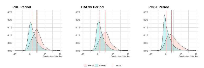
Figure 8: Density Plots for Deviations from Valid Rent
Notes: Deviations are computed as the difference between the valid rent and the advertised rent per square meter including
permitted overshooting by 20%. Periods are defined as in Table 5. Only observations with a start and end date in the same period
are allocated to the respective periods.
Acknowledging these shortcomings, we compute deviations (in EUR) conservatively via
Deviation = Advertised Rent per m2 − 1.2 · Valid Rent per m2 .
In other words, we include a potential error margin of 20% as such kind of over-shooting is
24Table 6: Percentage Deviation between the Advertised Rent and Valid Rent
PRE TRANS POST
Exempt from Rent Freeze
Deviation
Mean 4.17 4.62 4.16
Median 4.41 4.40 3.56
Q10 0.18 0.45 0.36
Q25 2.29 2.31 1.19
Q75 6.17 6.43 6.24
Q90 9.95 10.5 11.40
Interquartile Range 3.88 4.12 5.05
Covered by Rent Freeze
Deviation
Mean 1.78 0.88 0.77
Median 1.09 1.56 -0.11
Q10 -1.40 -1.38 -1.96
Q25 -0.35 -0.41 -1.15
Q75 3.24 2.92 1.92
Q90 7.63 7.16 6.62
Interquartile Range 3.58 3.07 3.25
Number of Observations 31,672 30,738 6,478
Notes: Deviations are computed as the difference between the valid rent and the advertised rent per square meter including
permitted overshooting by 20%. Periods are defined as in Table 5. Only observations with a start and end date in the same period
are allocated to the respective periods.
explicitly allowed. Overall, we hence are likely to identify the upper bound of the number of
dwellings exceeding the maximum allowed rent. Also, the amount of mismatches in EUR is, per
construction, an upper bound. We compute deviations separately for the three different periods
in order to detect systematic deviations. Also, we do so separately for properties covered by
the rent freeze and those exempt.
Table 6 and Figure 8 report the results. As expected, units exempt from the rent freeze
generally do not comply to the price restrictions binding for those covered. Most importantly,
the regulated dwellings advertised in the POST period by large means do not follow the re-
strictions imposed by the by-then legally binding rent freeze. Only roughly 50% are indeed
negative indicating a lower advertised rent than the valid rent. Put differently, only about half
of all advertisements do indeed follow the rules. Yet, the absolute difference in mean/median
25deviations between covered and exempt units is larger in the TRANS and POST periods than
in the PRE period indicating an increase in the degree of homogeneity in asking rents. Impor-
tantly, the lower the rent quintile, the more negative are the deviations between the advertised
and the valid rent, especially after the enactment of the rent freeze. This means that the freeze
is more effective in the affordable rent segment.
Importantly, asking rents are per definition not restricted – only realized rents indeed are.
Yet, such information likely induces confusion and potentially animates to tricking tenants
unaware of how to exactly compute a valid rent. Particularly the last point raises concerns
whether complex laws affecting the vast majority (Germany-wide homeowner rate is 46.5%,
while that in Berlin is only 17.4%)20 should in fact be designed in such complex terms. The
provision of easy-to-handle automatic valuation and evaluation tools may be necessary.
5.5.2. Regional Variation
We assess regional variation in coverage and compliance rates. Therefore, we compute key
measures separately for each of the Berlin’s 12 districts (see Table 7). Again, we focus on
advertisements activated after the rent freeze’s enactment.
On average, 83% of all advertisements posted are covered by this policy. The district-specific
shares, however, reveal substantial variation: between 67% in Friedrichshain-Kreuzberg and
95% in Spandau.
We further compute average deviations of posted rents from the valid rent. Table 6 re-
ports the overall figures for covered units and finds large deviations after the rent freeze’s
enactment. Looking at Berlin as a whole, roughly 50% of all ads followed the restrictions.
Again, the regional variation is substantial: While more than 50% of advertised rents fol-
low requirements in Charlottenburg-Wilmersdorf, Lichtenberg, Marzahn-Hellersdorf, Spandau
and Treptow-Köpenick, the large deviations are, in fact, driven by advertisements referring to
units located in the affluent central districts Friedrichshain-Kreuzberg and Mitte, as well as
the traditionally affluent district Steglitz-Zehlendorf in the South-West of Berlin (see Table 16
in Appendix for district-specific demographic information). In part, these regional differences
20
See the homeownership rate statistics (Eigentümerquote nach Bundesländern im Zeitvergleich) of the Fed-
eral Statistical Office of Germany; https://www.destatis.de/DE/Themen/Gesellschaft-Umwelt/Wohnen/
Tabellen/eigentuemerquote-nach-bundeslaender.html.
26Table 7: Variation after Enactment across Districts
Coverage Rate Median Rent Deviation
of Covered Ads
[%] [EUR]
Charlottenburg-Wilmersdorf 83.59 -0.111
Friedrichshain-Kreuzberg 66.85 2.608
Lichtenberg 73.58 -1.071
Marzahn-Hellersdorf 82.80 -0.868
Mitte 71.36 1.286
Neukölln 90.07 0.161
Pankow 82.90 0.282
Reinickendorf 92.29 0.002
Spandau 94.85 -0.778
Steglitz-Zehlendorf 92.04 0.636
Tempelhof-Schöneberg 87.68 0.138
Treptow-Köpenick 74.79 -0.410
Overall Mean 82.73 0.156
Overall Median 83.25 0.070
Notes: The table reports key figures by district: Rent Freeze Coverage Rates (number of ads covered by rent freeze over all posted
ads), Median Deviation of Advertised Rents (per square meter) from Valid Rents. Overall means and medians are calculated across
district-specific values. Numbers refer to advertisements posted and closed between 23 February and 30 June 2020.
Sources: Authors’ calculations based on rent advertisements collected by Empirica Systeme.
can be explained by an inaccurate representation of location in the Mietspiegel that does not
capture the actual spatial effects, as noted by Kauermann and Windmann (2016); Rendtel and
Frink (2020). Indeed, the average location in the city center is not worth the same as the aver-
age location at the periphery. Thus, the Mietspiegel tends to undervalue the dwellings located
in the center and overvalue those located at the periphery.
6. Robustness Checks
6.1. Alternative Control Group
An alternative specification of the control group includes all apartments that were built or
offered for first-time occupancy (either in newly built or substantially refurbished flats) after
1 January 2014. This classification is less strict since it might also cover relatively old flats
that are nonetheless offered for first-time occupancy. We re-estimate the main results for this
27You can also read