Frequency response function shape differences as a sign of bricks elements destruction diagnostics
←
→
Page content transcription
If your browser does not render page correctly, please read the page content below
MATEC Web of Conferences 332, 01021 (2021)                     https://doi.org/10.1051/matecconf/202133201021
19th International Conference Diagnostics of Machines and Vehicles

      Frequency response function shape differences
      as a sign of bricks elements destruction
      diagnostics
      Mariusz Żółtowski1,* and Raimondas Šadzevičius2
      1Warsaw   University of Life Sciences – SGGW, 02-787 Nowoursynowska 166, Poland.
      2Vytautas Magnus University Agriculture Academy, 53361 Kaunas, Lithuania.

                    Abstract. The knowledge of the dynamic state and structure of system
                    allows describing its behavior and allows creating prognosis models of the
                    system behavior in the function of dynamic evolution time, based on the
                    model of the technical state symptoms growth. Most often, there are no
                    known equations describing behaviors of the system in the function of
                    dynamic evolution time, which accounts for the need to apply new tools to
                    examine the dynamic state. In this article authors shows chosen problems
                    of technical state diagnosis with the use of identification and technical
                    diagnostics methods such as experimental modal analysis. Relations
                    between methods of dynamic state evaluation and methods of technical
                    state evaluation were indicated. Example modal analysis results illustrate
                    the complexity of projecting dynamic state researches into diagnostic
                    researches of state evaluation.

      1 Intorduction
      Destruction processes of technical systems force the need to supervise changes of their
      technical state. It is possible with the use of technical diagnostics methods.
          Methods and means of modern technical diagnostics are a tool of machine state
      diagnosis, which is the basis of decisions made at each stage of their existence.
          Many previous works clearly indicate connections between dynamics and technical
      diagnostics, especially vibration diagnostics. The bases of identification, modeling and
      concluding fully convince towards the dominating role of vibrations in machine state
      identification [1]. Properly planned and realized experiment is the base to obtain
      diagnostically sensitive signals, which processed will determine state diagnosis procedures.
      The processing includes creation of numerous signal measures in time domain, frequencies
      and amplitudes, selection and reduction of the number of signal measures, creation and
      analysis of effectiveness of cause-and-effect models, as well as evaluation of the
      righteousness of made diagnostic decisions [2].
      2 Dynamics and diagnostics
      Into quality measures of machine’s technical state, i.e. its dynamics, included is the level of
      vibration amplitudes, as well of the machines as the lot, and also of relative vibrations of
      separate elements and parts. Overall vibrations of the machine can be perceived as an
      external symptom while they are responsible for the level of interferences emitted into the
      environment. Relative vibrations of separate elements, however, influence mainly the state
      of internal forces in the machine, i.e. at its level of dynamic stress amplitudes [3].
          Identification can concern both the construction of models and the reconstruction of the
      examined model state, which leads straight to the problem of technical diagnostics.

      * Corresponding author: zoltowskimariusz1981@gmail.com

© The Authors, published by EDP Sciences. This is an open access article distributed under the terms of the Creative Commons
Attribution License 4.0 (http://creativecommons.org/licenses/by/4.0/).
MATEC Web of Conferences 332, 01021 (2021) https://doi.org/10.1051/matecconf/202133201021
19th International Conference Diagnostics of Machines and Vehicles
The process of diagnostic identification includes modeling (symptom or structural),
identification experiment (simulation and/or real), estimation of diagnostic parameters
(state features or symptoms), diagnostic concluding. The specificity of diagnostic
identification tasks is different from general identification in the way that it includes a
number of additional elements enhancing this process. They are:
• constructing models of diagnostic signals generation,
• choosing features of object structure state and diagnostic symptoms,
• modeling cause-and-effect relations,
• evaluating the accuracy of choosing variables for the model,
• determining boundary values of the symptoms,
• state classification and determining of periodicity a diagnosis.
Methods of identification can be divided concerning: the kind of identified model, the
kind of experiment, identification criterion applied, as well as estimation procedure applied.
In general, these are: methods of analysis, time, frequency, correlation, regression, factor
analysis, as well as iteration methods described in works of many authors [4].
For simple objects a good tool to evaluate their changeable dynamic state are methods
of simple identification, which use amplitude - frequency spectrum. Searching resonance
frequency and amplitude value in this frequency with the use of tests (impulse, harmonic
and random) are relatively well mastered in research techniques of our enterprises [5].
Another way of describing and analyzing the dynamic state of machines is a modal
analysis used as a theoretical, experimental and exploitation method. It uses frequencies of
own vibrations, values of suppression and forms of vibrations to describe the changing
machine state, and it is used to improve the finished elements method. The presented
procedures are based on the knowledge of the system model, and the conclusions drawn
from the actions on the models depend on their quality. Depending on the aim of the
performed dynamic analysis of the object, different requirements are set for the constructed
models, and their evaluation is conducted with different experimental methods.
3 Description of object state changes
The dynamic state of the object can be, in the easiest case, described with a model of 1
degree of freedom – Fig.1. A conventional description of this model is known relations
indicating that vibrations well reflect the state of the machine. A description of this model
can be achieved within m, k, c categories, or through a, v, x researches [6].
k c
Fig.1. System model of 1 degree of freedom and vibration signal of real system.
“the state parameters (m, k, c) = vibration process (a, v, x)”
(1)
x = A sin( t + ) (2)
dx
v= = A cos(t + ) (3)
dt
d 2 x dV
a= = = − A 2 sin(t + ) (4)
dt 2 dt
2MATEC Web of Conferences 332, 01021 (2021) https://doi.org/10.1051/matecconf/202133201021
19th International Conference Diagnostics of Machines and Vehicles
Identification of his model (Eq.1) from the experimental side is the a, v, x measurements
for different time moments, which reflects the changes of the object state and is widely
applied in vibration diagnostics. The solution of the task in the m, k, c, categories, however,
requires a number of solution conversion of the equation (Eq. 1) for determining:
c kr = 2m c kr = 4 mf
(5)
k = m 2
k = 4 mf 2 2
(6)
Determining the value (5) requires realizing identification experiment from which the
frequency f or frequency ω can be determined. Here is useful the simple identification or
modal analysis directly giving the values of own frequencies ω from the stabilization
diagram – Fig. 2.
Fig.2. Stabilization diagram for ω determination.
The problem becomes more complicated for models of many degrees of freedom (more
than 3). Here also the problem of object state identification can be solved from the
measurement side (a, v, x), Chile from the side of determining m, k, c own problem needs
to be solved [7].
(K − 2
)
M q0 = 0 (7)
Equation (Eq. 3) presents a linear system of homogeneous algebraic equations:
(k11 ) ( ) (
− 2 m11 q1 + k12 − 2 m12 q2 + + k1n − 2 m1n qn = 0 )
(k 21 − 2 m21 )q + (k
1 22 − 2 m22 )q 2 + + (k 2n − 2 m2 n )q n =0
…… ……. ……. …… (8)
A solution for q 0 exists when the main matrix determinant ( K − ω M ) = 0 , i.e.
2
det( K − ω2 M ) = 0 Solving the system of Eq. 4 own values can be determined, and from
.
them the frequencies of own vibrations, indispensable for the object identification.
k
λ = ω =
2
m (9)
3.1 Environment of experimental modal analysis
For complex systems, nonlinear often used for identifying complex modern method of non-
invasive test, which is the modal analysis. As a result of modal analysis is obtained modal
3MATEC Web of Conferences 332, 01021 (2021) https://doi.org/10.1051/matecconf/202133201021
19th International Conference Diagnostics of Machines and Vehicles
model, which is an ordered set of its own frequency, the corresponding damping ratios and
mode shapes. Based on knowledge of the modal model of the object can be predicted
response to any disorder in both time and frequency domains [8].
Using the statement that the destruction of the state of the object (test material) can be
described alternatively [instead of modelling the changes in terms of the (m, k, c) use the
description of the vibration in terms of (a, v, x)] in the study of the development of the state
of degradation of the structure or masonry vibration frequencies were evaluated, resulting
directly from the application of modal analysis procedures [9].
The identification of the individual modal models for extortion in the test sub-element
and further aggregating them for the whole structure of the object is obtained evolutionary
model, clearly describing the changes estimators state variable load conditions. Is revealed
by the fractal nature of energy conversion the processes, and perfecting possible ways to
zoom description of the real world. In most practical applications require the analysis of a
multi-modal experiment and the complex calculations associated with the processing of the
measured signals and model parameter estimation. So, welcome the possibility of
applications allows us to distinguish the following types of modal analysis:
• theoretical MA, which requires the solution of the problem for the assumed its
structural model of the object,
• experimental MA, controlled experiment requiring identification, during which
forces the movement of an object (eg. Vibrations) and measures the force and
measure the responses in a number of measuring points distributed over the
examined object,
• operational (exploitation) MA, based on a real experiment, in which measurements
are made only in response to the many points of measurement, while the
movement of the subject is due to the actual operating extortion.
The theoretical modal analysis is defined as the problem of self-dependent mass matrix,
rigidity and damping. The theoretical modal analysis requires addressing issues of their
own for the assumed of structural model. Here designated frequency sets its own frequency
attenuation coefficients for their own forms of vibrations and allow the simulation of
structural behaviour at any extortion, selection of controls, and other design modifications.
It is used in the design process, when there is no possibility of carrying out studies on the
subject. Modal analysis is widely applied resulting damages removing it from vibrations,
modifying structure dynamics, updating analytical model or state control, and also used for
monitoring vibrations in aircraft industry and civil engineering [9].
Theoretical modal analysis is defined as a matrix eigenvalue problem of dependent
matrices of mass, stiffness and damping. It requires the eigenvalue problems for an
Assumed structural model of investigated structure to be solved. The determined sets of
natural frequencies, damping coefficients for the natural frequencies and forms of natural
vibrations make it possible simulate behaviour of a structure under arbitrary excitations,
choice of steering means, modifications and other structural issues.
Analysis of natural frequencies and vectors is obtained on the basis of motion equations
(after neglecting terms which contain external damping matrix and load vector). Then the
motion equation of natural vibrations helps us obtains the form:
+Kq=0
Bq (10)
For one d.o.f. system its solution is as follows:
q
(t)=qsin(
t+) (11)
where:
- vector q of amplitudes of natural vibrations.
4MATEC Web of Conferences 332, 01021 (2021) https://doi.org/10.1051/matecconf/202133201021
19th International Conference Diagnostics of Machines and Vehicles
On substitution of the above given equation and 2nd derivative to the motion equation
the following is obtained:
−
( B
2
+
Kq
)
t+
sin(=
) 0 (12)
The equation is to be satisfied for arbitrary instant t, then the set of algebraic equations
is yielded as follows [14,19]:
(K−2B)q=0 (13)
This way was produced the set of linear homogeneous algebraic equations, which has
non-zero solution only when the condition is fulfilled:
K−
det(2
B)=0 (14)
On transformations the n-order polynomial is obtained. Among its roots multifold ones
may be present, and the vector built from the set of frequencies ϖ2 ordered according to
increasing value sequence is called the frequency vector, and the first frequency is called
the fundamental one [11]:
=[
1,
2....,
n] (15)
3.2 Experiment in modal analysis
Experiment to identify the state of the tested masonry destruction is the primary source
information and on the basis of measurement values can be determined and the structure of
the model. On the one hand, the quality of the experimental results obtained depends on the
quality of the model, on the other hand the way the experiment determines the structure of
the identified model [7].
The experiment of modal analysis can be divided into the following steps:
1) Planning the experiment:
• the choice of how to force vibration test piece and the points of application,
• selection of measurement points and vibration measuring equipment,
• selection of appropriate measuring equipment,
• selection of the model (reducing the number of degrees of freedom) of the
system.
2) Calibration of the measurement path.
3) Acquisition and processing of the results of the experiment.
The aim of the experiment is to force modal analysis of the movement of the test piece
masonry by providing energy and measuring the answer to extortion. The general procedure
for carrying out studies of this work is shown in Figure 3.
Fig.3. The essence of the measurement channel using modal analysis.
5MATEC Web of Conferences 332, 01021 (2021) https://doi.org/10.1051/matecconf/202133201021
19th International Conference Diagnostics of Machines and Vehicles
The test piece subjected to forcing the forced walled corresponds to the vibration signal,
proportional to the state of destruction. Forcing and response signal is used to determine the
function of further FRF and the stabilization of the diagram, and the frequency of
oscillations. By the way, these procedures are available for other interesting cognitive
processes vibration estimators, which are also used in further studies. Test results after
processing by different algorithms are subjected to statistical study. From the viewpoint of
experimental modal analysis methods can be divided into:
• a method of forcing movement of the multiple actuators for the excitation of one
form of vibration;
• the method of forcing movement of the one or more points in order to measure the
transfer function.
The first group of methods is carried out manually moving the system in such a way as
to force the vibration in accordance with one embodiment of the vibration. This requires a
complex control system actuator to obtain the appropriate phase shifts force. The second
group is used to force any depending on the type of the object. Set of equipment for the
implementation of the experiment modal analysis is made up of components:
• measurement of the force of motion and response measurement
• signal conditioning system (pre-processing),
• the processing and collection of signals,
• forcing signal generation system,
• the vibration excitation.
The simplest due to maintenance solution is to use signal analyser, but the most modern
giving the greatest potential solution is based on a workstation, and a specialized interface
measurement. The basic operation performed by all applicable devices measuring modal
analysis of signal to digital processing, which enables the use of digital signal processing
techniques to determine the modal analysis required by the characteristics of estimators.
Modal studies do not care that the size of the kinematic motion measuring, as a response
of the system. In practice, the displacement measurements give better results in terms of
low frequency, and acceleration of the high frequency range. It is widely believed that the
velocity measurements are the most optimal structural dynamics studies due to the fact that
the effective value of the vibration velocity is in some sense a measure of the kinetic energy
of vibration of the system. However, sensors for measuring displacement and velocity are
relatively heavy and may affect the behaviour of the test object and the acceleration sensors
have a considerably lower mass and therefore do not affect the motion of the system. An
additional advantage of the acceleration sensor is that the acceleration signal a further
signal can be obtained by integrating the velocity or displacement vibrations. Operation in
the opposite direction, which consists of differentiation, can lead to large errors, especially
in the higher frequencies.
On those grounds, acceleration sensors are the most commonly used transducers for
studies of modal structure. Acceleration sensors built on the piezo-electric phenomena can
be modelled as a system with one degree of freedom from suppression. The weight of this
model is the seismic mass aggravating crystal piezoelectric material during movement. Due
to the design of the sensors has its resonance, which reduces the frequency range in which
they can be applied.
A very important factor influencing the modal test results associated with a variety of
sensors, sensor-mounting location. The sensors should be mounted in such a way as not to
affect the vibration system and are secured at the characteristic behaviour of the structure.
Currently, the vibration measurement during the examination of the structure modal
contactless sensors, are used and one of the feasibility of this type of sensor is the use of a
laser beam. Such sensors enable the measurement of vibration velocity in the frequency
range of O to 50kHz, and amplitudes in the range of 0 to 100mm/s. An important factor in
6MATEC Web of Conferences 332, 01021 (2021) https://doi.org/10.1051/matecconf/202133201021
19th International Conference Diagnostics of Machines and Vehicles
the range of measured frequency of the sensor is no way for the study of the structure. The
sensors can be attached to the test structure by means of a special wax, adhesive, magnet or
screw with the screw.
Experimental modal analysis requires laboratory conditions for testing. Model is subject
to advance well-known and established extortion. Forcing these may differ from those that
operate on the object during normal operation. During the execution of the experiment may
encounter difficulty in keeping in line with the reality of such boundary conditions, for
example method of fixing the test object. In the case of large models, the execution of the
experiment is very expensive and often impossible.
4 Measurement software, and results
For the measurement waveforms extortion and response system and determine the most
used functions FRF measurement equipment purchased for the project company under the
name of LMS TEST.XPRESS. This software enables you to easily perform a modal
analysis of brick elements, as well as any other building structures. For the purposes of
measurement using experimental modal analysis you defined two measurement channels.
According to the theoretical experimental modal analysis first sensor is reserved for the
modal hammer (vibration force), and second piezoelectric sensor is connected on the wall
element (the answer key to force).
The next step was to prepare the masonry. In the study, it was decided to check is it
possible to see a difference in destruction state in bricks, with use of only FRF function. For
this purpose, were use 2 types of the samples. First sample was a full brick obtained from
the brickyard, and for comparison a cracked (seen cracks on surface) full brick were also
measured. For a better visualization of the results of the investigation, the results are shown
below separately - 5 times is shown the FRF function for good, and 5 times for destroyed
brick element. In Figure 4 it is shown once the extortion, and the answer of signal in time
domain, which allows gaining FRF function.
FRF – (Frequency Response Function) can be described as a quotient of the Fourier
transform vibration exciting force F(ω), the Fourier transform of the response signal A(ω).
Extortion Answer
FRF
Fig. 4. Composition of results of measurements (the temporary course of extortion, temporary course
of answer, function the FRF) the full brick in axis X.
During the tests it was able to generate a transfer functions of vibration signal by the
structure (FRF function). The results are presented in real time in the center of a screen. It’s
allows visualizing the temporary courses of extortions and the answer, as well as the
function the FRF and the function of coherence.
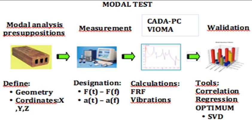
Graphic results, which show FRF functions of good, and destroyed bricks measured in
axel Y and 6 measurements for each material sample are show below in figure 5.
7MATEC Web of Conferences 332, 01021 (2021) https://doi.org/10.1051/matecconf/202133201021
19th International Conference Diagnostics of Machines and Vehicles
60
40
dB/1 [(m/s2)/N]
40
dB/1 [(m/s2)/N]
20
20
0 0
-20 -20
-40 0 1000 2000 3000 4000 5000 6000
0 1000 2000 3000 4000 5000 6000 Frequency Traces: 1/1 Compressed Frequency [Hz]
Frequency Traces: 1/1 Compressed Frequency [Hz]
40 40
dB/1 [(m/s2)/N]
30
dB/1 [(m/s2)/N]
20 20
10
0
0
-10 -20
-20
0 1000 2000 3000 4000 5000 6000 0 1000 2000 3000 4000 5000 6000
Frequency Traces: 1/1 Compressed Frequency [Hz] Frequency [Hz]
Frequency Traces: 1/1 Compressed
60 40
dB/1 [(m/s2)/N]
40
20
dB/1 [(m/s2)/N]
20
0
0
-20 -20
-40
0 1000 2000 3000 4000 5000 6000 -40
Frequency Traces: 1/1 Compressed Frequency [Hz]
0 1000 2000 3000 4000 5000 6000
60 Frequency Traces: 1/1 Compressed Frequency [Hz]
40 60
dB/1 [(m/s2)/N]
20 40
dB/1 [(m/s2)/N]
0 20
-20 0
-40 -20
0 1000 2000 3000 4000 5000 6000
Frequency Traces: 1/1 Compressed Frequency [Hz] 0 1000 2000 3000 4000 5000 6000
Frequency Traces: 1/1 Compressed Frequency [Hz]
60
40 40
dB/1 [(m/s2)/N]
dB/1 [(m/s2)/N]
20 20
0
0
-20
-20
-40
-40
0 1000 2000 3000 4000 5000 6000 0 1000 2000 3000 4000 5000 6000
Frequency Traces: 1/1 Compressed Frequency [Hz] Frequency Traces: 1/1 Compressed Frequency [Hz]
Fig. 5.Composition of FRF functions of full brick (good -left, damaged – right) in axis Y.
The results clearly differentiate the state of bricks degradation and in further research to
indicate the usefulness of FRF be determined limit states in industrial diagnostic research.
5 Summary
Sulfur concrete is prepared hot by mixing modified sulfur cement and additives. Methods
of identification in the research building construction (including construction materials) are
utility methods to estimate changes in operating structure. Civil engineers are increasingly
using modal analysis of the varieties for its realization and modal model accurately reflects
the destruction of objects.
Searching for mapping models with models of modal vibration, bench research and
studies on real objects, allows assessing the similarity of the models, the relevance and
effectiveness of decision methods. The search for methods of non-destructive testing of
materials and structures indicates the possibility of using modal analysis in the assessment
of their degradation, as shown in this study.
Practically verified susceptibility modal analysis of the degree of degradation of
masonry shows to the satisfaction of practice differences between of the structure can bear
and damaged. It is therefore possible to determine the risks of building structures on the
basis of the study of natural frequencies and their characters, using operational modal
analysis.
The results point to the fact that it is possible to distinguish between material properties,
which has an impact on the ability to distinguish between their mechanical properties. The
study also confirmed the usefulness of the LMS test apparatus using operational modal
analysis performed on the actual building construction.
By obtaining graphical charts of FRF function, and a later their comparison it is possible
to observe their diversity. These charts are different for materials that are in good condition,
and damaged, which demonstrates the ability to assessment of the destruction of a brick
element.
8MATEC Web of Conferences 332, 01021 (2021) https://doi.org/10.1051/matecconf/202133201021
19th International Conference Diagnostics of Machines and Vehicles
It practically verified the sensitivity of assessment of modal analysis to degree of brick
structure degradation. It becomes possible to determine hazards to a building structure on
the basis of examining values of frequencies.
References
[1] B. Żółtowski, M. Żółtowski, Vibration signals in mechanical engineering and
construction, (ITE-PIB 2015)
[2] B. Żółtowski, C. Cempel, Engineering of diagnostics machines, (PTDT, ITE – PIB
2004)
[3] M. Żółtowski, B. Żółtowski, Vibrations signal to the description of structural damage
of dynamic the technical systems, (XIII International Technical Systems Degradation
Conference 2015)
[4] M. Żółtowski, Opis drganiowy konstrukcji budowlanych, Logistyka nr.6/2014 (2014)
[5] M. Żółtowski, Investigations of harbor brick structures by using operational modal
analysis. Polish Maritime Research, No. 1/(81), vol. 21 (2014)
[6] M. Żółtowski, M. Liss, The use of modal analysis in the evaluation of welded steel
structures, Studies and Proceedings of Polish Association for Knowledge
Management, Vol. 79 (2016)
[7] M. Żółtowski, M. Liss, Zastosowanie eksperymentalnej analizy modalnej w ocenie
zmian sztywności prostego elementu konstrukcyjnego, Studies and Proceedings of
Polish Association for Knowledge Management, Vol. 80 (2016)
[8] M. Żółtowski, R.M. Martinod, Technical Condition Assessment of Masonry Structural
Components using Frequency Response Function (FRF), Masonry International
Journal of the International Masonry Society, Vol. 29, No.1, (2016)
[9] M. Żółtowski, R.M. Martinod, Quality identification methodology applied to wall-
elements based on modal analysis, Civil Engineering the Athens Institute for
Education and Research, Emerald, Athens (2015)
9You can also read