The GBT Sensitivity Calculator User's Guide - Dan Perera Ron Maddalena - July 5, 2013
←
→
Page content transcription
If your browser does not render page correctly, please read the page content below
The GBT Sensitivity
Calculator User’s Guide
          Dan Perera
        Ron Maddalena

          July 5, 2013
ii

Table of Contents
1.     Introduction to the GBT Sensitivity Calculator ............................................................................................................... 1
     1.1      How Start the GBT Sensitivity Calculator ................................................................................................................ 1
2.     Structure and Common Features of the Sensitivity Calculator....................................................................................... 2
     2.1      Structure ................................................................................................................................................................. 2
     2.2      Features .................................................................................................................................................................. 3
3.     General Information Frame ............................................................................................................................................ 3
     3.1      Observing Time from Desired Sensitivity ................................................................................................................ 3
     3.2      Sensitivity from Observing Time ............................................................................................................................. 4
4.     Hardware Information Frame ......................................................................................................................................... 4
5.     Source Information Frame .............................................................................................................................................. 6
6.     Data Reduction Frame .................................................................................................................................................... 7
7.     Results Frame .................................................................................................................................................................. 9
     7.1      Controls ................................................................................................................................................................... 9
     7.1      The Results Window ............................................................................................................................................... 9
       7.1.1          The Grid Results Tab ..................................................................................................................................... 11

Appendix
      A. Definition and Terms ……………………………………………………………………………………………….……………………………………….11
      B. Basic Equations ........……………………………………………………………………………………………………………………...…………………13
      C. 1/F Gain Instabilities ………………………..………………………………………………………………………………………….……………………16
      D. Confusion Limit .………………………………………………………………………………………………………………………….…….………………16
      E. Determining Various Quantities .……………………………………………………………………………………………………………………….17

References…..……………………………………………………………………………………………………………………………………………………..….22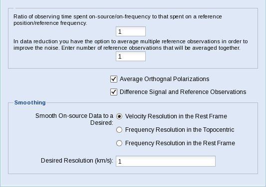
1. Introduction to the GBT Sensitivity Calculator

The new GBT Sensitivity Calculator has been designed to provide observers an easy way to determine the time needed
to complete a proposed project or the expected sensitivity achieved by a project of a given length. In comparison with
our previous calculator, the replacement is significantly more sophisticated and leads users through a complex web of
decisions and choices astronomers make as they think out their sensitivity estimates. The new calculator should simplify
the writing of a proposals technical justification since a user can save the input parameters and results to a file which
can then be attached to a proposal. Since an attachment will contain very complete details, it will also reduce the
chance that a reviewer will misinterpret the technical justification.

The calculator has been designed to satisfy 95% or so of ‘traditional’ spectral line, pulsar and continuum observations
and is not guaranteed to produce results better than 10% in sensitivity or 20% in time. It is up to the user on how best
to derive from the calculator’s output the total time for their sessions and projects. Thus, we expect those writing
proposals to continue to use the technical justification section of their proposals to describe how the results of the
calculator were used to derive the time estimates for their projects. Users can also include in their technical
justifications as many output logs from the calculator as they feel are needed.

This document has been compiled to guide users through the flow of questions asked by the calculator in order to
produce a final sensitivity or time estimate which can then be included in the technical justification of the proposal. The
structure and common features of the sensitivity calculator can be found in Chapter 2. The following chapters are
devoted to separate frames within the sensitivity calculator that require user input and should each be completed
sequentially.

3.   General Information
4.   Hardware Information
5.   Source Information
6.   Data Reduction
7.   Results

The Appendix provides a detailed discussion of the parameters and equations used by the calculator.

1.1 How Start the GBT Sensitivity Calculator

The Sensitivity Calculator is located at https://dss.gb.nrao.edu/calculator-ui/war/Calculator_ui.html. You will need to
supply your ‘My NRAO’ username and password.
2
2. Structure and Common Features of the Sensitivity Calculator
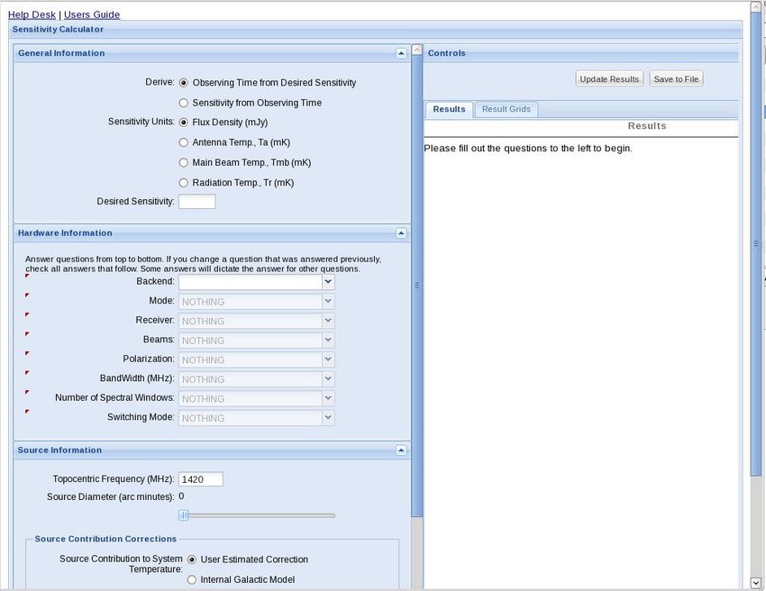
When you first start the GBT Sensitivity Calculator you will be presented with the screen shown in Figure 2.1.
Figure 2.1: The GBT Sensitivity Calculator
2.1 Structure
The GBT Sensitivity calculator has been designed in a way that guides the user through various sequential steps. In
general you should start by completing boxes from top to bottom, as the questions asked of you will depend on your
answers to previous questions. For example, you will not be asked how many beams you wish to use if you have
selected a single beam receiver. Any questions that are not applicable to your proposed observations or that cannot be
asked at an early stage will be grayed out. As you select your answer to a question, the calculator will automatically
update and if necessary, further questions may be asked of you.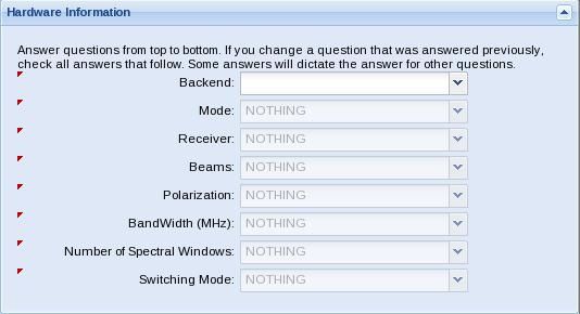
3

Questions asked of the user are organized by topics given in the frames on the left hand side of the screen (General
Information, Hardware Information, Source Information and Data Reduction). At any time you may press the ‘Update
Results’ button to view any parameters that the calculator can return to you based on the answers you have given. If
the calculator is not able to return a derived sensitivity or total observing time then you still have some questions to
answer.

2.2 Features

•   Help Desk – You may select this link to send an email to the Dynamic Scheduling System (DSS) helpdesk using your
    default email application.
•      – Press the up arrow button to minimize its associated frame.
•      – Press the down arrow button to expand its associated frame.
•      – Red triangles denote questions that must be answered in order for the calculator to proceed or denote fields
    that have been altered, requiring you to press the ‘Update Results’ button on the right side of the calculator.

3. General Information Frame

You must select whether you wish to derive the total observing time from a given sensitivity or vice versa. In either
case, you must first need to choose your units for sensitivity. The allowed units are:

    •   Flux Density (mJy) - (10 Watts m Hz  ), and as if measured from above the Earth’s atmosphere (Default).

    •   Antenna Temp., Ta (mK) - as measured below the Earth’s atmosphere.

    •   Radiation Temp., Tr (mK) - as if measured from above the Earth’s atmosphere and defined for sources of any
        size.

    •   Main Beam Temp., Tmb (mK) – similar to Tr, but defined for sources whose diameter extends to the first nulls in
        the telescope’s beam.

3.1 Observing Time from Desired Sensitivity

Enter the sensitivity that you wish to achieve in the Desired Sensitivity box in your chosen units.
4

                   Figure 3.1: General Information Frame - Observing Time from Desired Sensitivity

3.2 Sensitivity from Observing Time
Enter the total time required for your observations. Units of time can be entered in seconds or sexegesimal format.

                       Figure 3.2: General Information Frame - Sensitivity from Observing Time

4. Hardware Information Frame
You will be asked a series of questions concerning your choice of hardware and the calculator will check the answers to
make sure that they can be accommodated by the hardware. Only those questions needed for the sensitivity calculator
will be asked. For example, if you select MUSTANG as your backend, then all subsequent choices will be filled out for
you with the MUSTANG default values, and you will not be required (or able) to answer any further questions within this
frame.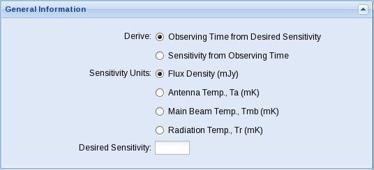
5

                                       Figure 4.1: Hardware Information Frame

The available fields within the Hardware Information Frame are:

   •   Backend – You may currently choose from the following backends:
           Caltech Continuum Backend (CCB)
           GBT Digital Continuum Receiver (DCR)
           GBT Spectrometer
           Green Bank Ultimate Pulsar Processor (GUPPI)
           Mustang
           Spectral Processor
           VErsitile GB Astronomical Spectrometer (VEGAS)
           Zpectrometer

   •   Mode – This will be selected automatically depending on your choice of backend. The available modes currently
       available for each backend are:
            Continuum – CCB, DCR, VEGAS and Mustang
            Spectral Line – VEGAS, GBT Spectrometer, Spectral Processor and Zpectrometer
            Pulsar – VEGAS, GUPPI

   •   Receiver – If you have selected VEGAS, DCR, GBT Spectrometer or Spectral Processor as your backend then you
       will need to select which GBT receiver your wish to use.

   •   Beams – If the receiver you have selected is capable of using more than one beam then you will be prompted to
       enter how many beams you wish to use here.

   •   Polarization - You will be given a choice between Dual and Full for the GBT Spectrometer and FPGA
       Spectrometer, and between Cross_QU, Dual and Full with the Spectral Processor.
6
• Bandwidth – You may be given a choice of available bandwidths depending on which backend you have
selected.
• Spectral Windows – You may be given a choice of how many spectral windows you wish to use for your
observations.
• Switching Mode – Currently you may choose between ‘In-Band Frequency Switching’, ‘Out-of-Band’ Frequency
Switching’ and ‘Position Switching’.
5. Source Information Frame
Since projects usually observe multiple sources, you may want to run the sensitivity calculator for each, but it is also
acceptable to run the calculator for a representative source, or a representative set of source parameters. If the latter
approach is taken then you will need to infer how that calculation for a single or representative source translates into
the time or sensitivity requirements for the body of your sources.
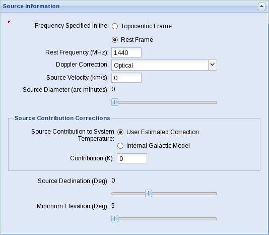
Figure 5.1: Source Information Frame
User input is required for the following fields:
• Topocentric Frame / Rest Frame – You will be asked if the observing frequencies will be given in the line’s reset
frame or in the topocentric frame. The default is ‘Rest Frame’
• Topocentric / Rest Frequency (MHz) – The default will be the middle of the selected receivers band.7
• Doppler Correction – If you had previously selected ‘Rest Frame’ then you will be asked to select between an
optical, radio and redshift Doppler correction. The default is ‘Optical’.
• Source Velocity (km/s) / Redshift - Depending on the selected Doppler correction you will be asked to supply a
representative source velocity or redshift. The default in either case is zero.
• Source Diameter (arc minutes) – Use the slider to set a representative size for your source. Available values
range from 0 (point source) to the FWHM of the GBT beam. The calculator assumes the source brightness
distribution is that of a uniform disk. The slider is not available is you have selected units of Ta or Tmb as the
definitions of these conventions include a predefined source size.
• Source Contribution Corrections – You will be asked whether to apply a correction for the representative
source’s continuum level to the calculator’s system temperature calculations. The options are:
User Estimated Correction – If you select this options then you will be asked to provide the background
level in the units that you have selected in the ‘General Information’ frame.
Internal Galactic Model – If selected then the calculator will ask for a representative J2000 Right
Ascension of the source. The calculator will then augment the system temperature with the
approximate continuum background from the Milky Way for the specified position using the 408 MHz
survey of Haslam et al (1981, A&A, 100, 209)
• Source Declination (Deg) – Use the slider to set a representative source Declination in degrees (default = 0°).
• Minimum Elevation (Deg) – Use the slider to set the minimum allowable elevation for observations of the
source (default = 5°). The calculator will provide a suggested minimum elevation, dependent on your source
declination and observing frequency, if the value you entered is less than the recommended value.
6. Data Reduction Frame
Observers have a number of choices in how they collect and reduce their data that significantly affect the time they will
need for an experiment and the corresponding sensitivity they will achieve. Only those that are most common have
been included in the calculator.8
Figure 6.1: Data Reduction Frame
The available fields available for data reduction depend upon your answers in the hardware frame. Possible questions
include:
• Ratio of observing time spent on-source/on-frequency to that spent on a reference position/reference frequency
– If you have selected any switching mode other than total power, then you will be asked:
The ratio of time spent on your signal (on-source or on-frequency) observation to their reference
observation. The default is set to 1.
The number of reference observations that will be averaged together. The default is set to 1.
• Average Orthogonal Polarizations – You will be offered this choice based on your hardware configuration. If
applicable then this box will be checked by default.
• Difference Signal and Reference Observations – You will be asked whether you plan on differencing signal and
reference observations. By default this is set to on.
• Smoothing – For spectral line observations you will be required to provide how you will smooth both the on-source
and off-source data and whether you will be smoothing to a specified:
Velocity Resolution (km/s) in the source’s rest frame (default)
Frequency Resolution in the Topocentric Frame (MHz)9
Frequency Resolution in the Rest Frame (MHz)
• Resolution – Enter the desired resolution in the units selected above (Default = 1).
7. Results Frame
The results frame on the calculator’s right side is where all the output from the sensitivity calculator will be displayed.
Figure 7.1 shows the results frame prior to any entries by the user.
Figure 7.1: A Blank Results Frame
7.1 Controls
The only interface with the results frame is through the two buttons under ‘Control’.
• - Press the ‘Update Results’ button to display all results that the sensitivity calculator can currently
return based on the information you have given. The calculator will also prompt you to press this button if you have
changed any of the entries in the user input frames on the left of the screen by displaying a red arrow next to any
field that has been altered.
• - If you press the ‘Save to File’ button then you will be given the option of saving the information
displayed in the results frame as a text file. The file can then be attached to your proposal.
7.1 The Results Window
The results grid is for debugging as it presents all of the internal variables and values used by the calculator’s underlying
code. The results tab provides the most user friendly way to look at your results. Figure 7.2 gives an example of the
‘Results’ tab layout after all information has been provided by the user.10
Figure 7.2: Results Frame – ‘Results’ Tab
Outputs from the sensitivity calculator in this mode are given under the following headings:
• Results – This section contains information that will be of use to you when writing your technical justification. If you
are unable to derive a final sensitivity or total observing time, then you will need to include additional information in
the user input frames to the left of the screen (and also remember to press the ‘Update Results’ button). You may
also find it helpful to look under the ‘User Input’ heading (Also in the results frame) and scan it for any fields which
appear to be blank, in which case you can enter that missing information in the relevant frame.
• Messages – Miscellaneous information that the calculator may deem important will be displayed under this section.
• Other Results – The values of constants used for the sensitivity calculators calculations. Details of these constants
and algorithms can be found in the Appendix.
• User Input – All of the information entered into the General Information, Hardware Information, Source Information
and Data Reduction frames will be displayed under this heading.11
7.1.1 The Grid Results Tab
Figure 7.3: Results Frame – ‘Result Grids’ Tab
If you select the ‘Result Grids’ tab, then the output will be displayed in table format (Figure 7.3). Unlike the ‘Results’ tab,
there are only two headings:
• Results – Contains all of the parameters that are given under the headings ‘Results’ and ‘Other Results’ in the Result
Tab.
• User Input – All of the information entered into the General Information, Hardware Information, Source Information
and Data Reduction frames will be displayed under this heading.
Appendix
A. Definition and Terms
Term Definition
Representative atmospheric attenuation, ∙ , for the typical weather condition and elevation of
A
an observation at the user’s observing frequency
AirMass Representative air mass through which the observations will be made
BW Bandwidth in MHz, either native to the backend or the bandwidth to which the user smoothes
BWRef Bandwidth in MHz that the reference (off) observation will be smoothed to
c Speed of light in m s-1
DishRadius Illumination radius for the selected receiver in m
∆fREST Frequency resolution in the rest frame in MHz
ΔVREST Velocity resolution in the rest frame in m s-1
ElMin, ElMax Range in observing elevation in °
EST Effective system temperature in K ( ∙ ∙ )
EST0 Effective system temperature under the best possible weather conditions12
Effective system temperature but augmented by the expect loss in efficiency due to tracking and
ESTTS
surface errors
FeedTaper Feed taper illumination of the reflector in dB.
Frequency Topocentric frequency in MHz
FWHM Full-width, half-maximum beam width in ‘
ηMB, ηl ηfss, Efficiency which takes into consideration surface errors as a function of frequency and source size for
and ηS various intensity conventions.
η0 Aperture efficiency at long wavelengths and receiver and frequency dependent
Aperture efficiency which takes into consideration surface errors as a function of frequency and
ηA
elevation
Normalized observing efficiency, in units of time, as suggested by DSS simulations and the product ηTrack
ηDss
ηSurf ηAtm
ηTrack, ηSurf, The normalized observing efficiency, in units of time, as suggested by DSS simulations due to tracking
ηAtm errors (e.g., wind induced), thermal-induced surface errors, and atmospheric conditions.
θSource Source size in ’
k Boltzmann’s constant
K1 Sampling sensitivity of a backend and, thus, is hardware dependent
Autocorrelation channel weighting factor for spectral line backends or a measure of the independence
K2
of samples for continuum observing; hence hardware dependent
Number of references observations that will be averaged together in the data reduction and used for
NRefAvrg
every signal (on) observation
Amount by which a reference observation is smoothed or the number of reference observations that
NRefSmthAvrg
are averaged together
Degree to which backend inputs measure uncorrelated signals. (For example, = 2 when averaging
orthogonal polarizations or when using nodding or in-band frequency switching )
RSigRef Ratio of time spent on the signal observation to the time on the reference observatio
∗!
Sensitivity in units of Jy (above atmosphere)
Sensitivity in K in the TR* (above atmosphere) temperature scale
# Sensitivity in K in the TA (below atmosphere) temperature scale
τ Representative zenith atmospheric opacity in units of Nepers
τ0 Best possible zenith atmospheric opacity in units of Nepers
Effective integration time in s - essentially the time that satisfies the radiometer equation and is related
teff
to the actual observing time in ways that depend upon the observing tactics
tSig Time spent in s on a source or signal position or frequency
tRef Time spent in s on a reference position or frequency
tTotal Total time in s needed to complete an observation
Temperature of the atmosphere in K to use in an estimate of TSys -- approximate temperature of the
TAtm
atmospheric layer that is contributing most to the opacity
TCMB The cosmic microwave background = 2.7 K
Either the continuum temperature in K of the user’s source or the temperature in K of the galactic
TBG
background in the direction of the observation
TRcvrl Contribution to TSys in K from the receiver
TSys Expected approximate system temperature in K at a representative elevation
V Source velocity in m/s
z Redshift (V/c)13
B. Basic Equations
The algorithms used by the sensitivity calculator are a modified version of the classic radiometer equation. The modified
equation describes the theoretical noise one would obtain if observing above the atmosphere with a given effective
system temperature (ESTTS ; see §E.1 for the relationship between ESTTS and TSYS) and bandwidth (BW in MHz) for a given
effective duration of an observation (teff in sec). If we ignore the contribution from 1/F noise:
) ∙ *+%, 1
$ %&∗ ' ( 0
-. -/
12,34
567899
∙ 10: ∙ ;< ∙ =eff
2,34
567899
depends upon the details of the observing tactics (§E.5). K1 = the sampling sensitivity of a backend (§E.3).
The calculator uses the definition of the TR* temperature scale of Kutner and Ulich (1981). Accordingly, TR* is the
brightness temperature of an equivalent black-body source with the assumption that the source is a circular disc of
uniform brightness. ηl ηfss corrects for both the efficiency of the telescope’s optics as well as the convolution of the
source brightness distribution with the telescope’s beam (§E.4).
Due to the rough accuracy needed, the calculator makes some simplifying assumptions:
• The Rayleigh-Jeans approximation holds at all frequencies,
• The ohmic-loss efficiency factors, ηr in Kutner and Ulich is taken to be equal to 1.
One should not use the results of the calculator for the accurate calibration of astronomical measurements.
Observers will be specifying (or requesting) sensitivities in the following units:
• Flux density (S in Jy = 10-26 Watts m-2 s-1), as if observed from above the Earth’s atmosphere
• Temperature as defined by the TA temperature scale, as observed from the surface of the Earth
• Temperature as defined by the TR* temperature scale, as if observed from above the Earth’s atmosphere
• Temperature as defined by the TMB temperature scale, which is identical to the definition of TR* but with the
assumption that the source size is the same as the telescope’s beam to its first null. Here, ηl ηfss is equal to the
standard definition of beam efficiency, ηMB.
With the above simplifying assumptions, and the standard conversions between these units of intensity, the
relationships of the theoretical noise for the various intensity scales are:
-, ∙ A ∙ BCDEFGHCID
$%@ ' ∙ $,
2K ∙ ∙
-. -/
$%@ ' ∙ ∙ $ %&∗
-M
$%@ ' ∙
∙ $%NO
∙
, hereafter called AtmosAtten, is the representative atmospheric attenuation for the elevation range
of the observation; k = Boltzman’s constant. Section E.4 describes how ηS, ηMB and ηl ηfss depend upon the efficiency
of the telescope’s optics and source size.14
Most observing tactics require differencing observations of a signal/source position (or signal frequency) with a
reference position (or reference frequency). Since both the signal and reference observations have noise, the resulting
difference will be noisier than either the signal or reference observation. Since teff is related to the noise in the resulting
difference, teff is always less than the total duration of the signal plus reference observation.
Often one may spend different amount of time on each phase of an observations. For example, to save overhead it’s
common practice to use one reference observation for multiple signal observations. The calculator defines RSigRef ,
which has a default value of 1, as the ratio of the time spent on each phase of an observation.
FSigRef ' =Sig ⁄=Ref .
To help reduce the extra noise from differencing observations, it’s a common practice during data analysis to smooth
the reference observation or to average multiple reference observations. The calculator defines RRefSmthAvrg , which has
the default value of 1, as the amount by which a reference observation is smoothed or averaged beyond any smoothing
done to the signal observation. From the theory of the propagation of errors, the noise in the difference is:
$ ' $,U
V $WX/
Assuming ESTTS is the same for the signal and reference observations, the above equation implies that:
1 1 1
' V
=eff =Sig FRefSmthAvrg ∙ =Ref
And, therefore,
=Sig ∙ ^FRefSmthAvrg ∙ =Ref _
=eff '
=Sig V^FRefSmthAvrg ∙ =Ref _
The typical user isn’t interested in the value of teff, tSig or tRef. Rather, users are mostly interested in the total duration
needed for an observation (tTotal). If there is no overhead involved in the observing, then tTotal = tSig+tRef, and after a bit of
algebra, one derives the following relationships between teff , tTotal, tSig and tRef:
dFSigRef V FRefSmthAvrg edFSigRef V 1e
=Total ' =Sig V =Ref ' =eff ∙
FSigRef ∙ FRefSmthAvrg
FSigRef ∙ FRefSmthAvrg
=eff ' =Total ∙
dFSigRef V FRefSmthAvrg edFSigRef V 1e
=,U ' =%fg. ∙ F,UWX/ ⁄dF,UWX/ V 1e
=WX/ ' =%fg. ⁄dF,UWX/ V 1e.
The above radiometer equations for the various intensity scales, in terms of tTotal, are then:15
2K ∙ ) ∙ *+%, dFSigRef V FRefSmthAvrg edFSigRef V 1e
$, ' i j k
- ∙ A ∙ BCDEFGHCID 10: ∙ ;< ∙ 2,34
567899
∙ FSigRef ∙ FRefSmthAvrg ∙ =Total
) ∙ *+%, dFSigRef V FRefSmthAvrg edFSigRef V 1e
$ %&∗ ' ( 0k :
-. -// 10 ∙ ;< ∙ 2,34
567899
∙ FSigRef ∙ FRefSmthAvrg ∙ =Total
) ∙ *+%, dFSigRef V FRefSmthAvrg edFSigRef V 1e
$% 'i jk :
NO -M 10 ∙ ;< ∙ 2,34
567899
∙ FSigRef ∙ FRefSmthAvrg ∙ =Total
) ∙ *+%, dFSigRef V FRefSmthAvrg edFSigRef V 1e
$%@ ' i jk :
l=mnDl== o 10 ∙ ;< ∙ 2,34
567899
∙ FSigRef ∙ FRefSmthAvrg ∙ =Total
Some observing tactics will not require taking a reference observation, which implies that tTotal=teff. In these cases:
2K ∙ ) ∙ *+%, 1
$, ' i j k
-, ∙ A ∙ BCDEFGHCID 10: ∙ ;< ∙ 2,34
567899
∙ =Total
) ∙ *+%, 1
$ %&∗ ' ( 0k :
-. -/ 10 ∙ ;< ∙ 2,34
567899
∙ =Total
) ∙ *+%, 1
$ %&∗ ' i jk :
-M 10 ∙ ;< ∙ 2,34
567899
∙ =Total
) ∙ *+%, 1
$%@ ' i jk :
l=mnDl== o 10 ∙ ;< ∙ 2,34
567899
∙ =Total
Simple inversions of these equations allow one to derive a total time from a user-supplied sensitivity:
2K ∙ ) ∙ *+%,
dFSigRef V FRefSmthAvrg edFSigRef V 1e
=Total ' i j ( 0
-, ∙ A ∙ BCDEFGHCID ∙ $,
;< ∙ 2,34
567899
∙ FSigRef ∙ FRefSmthAvrg
dFSigRef V FRefSmthAvrg edFSigRef V 1e
) ∙ *+%,
=Total '( 0 ( 0
-. -/ ∙ $ %&∗ ;< ∙ 2,34
567899
∙ FSigRef ∙ FRefSmthAvrg
) ∙ *+%, dFSigRef V FRefSmthAvrg edFSigRef V 1e
=Total 'p q ( : 0
-M ∙ $ % 10 ∙ ;< ∙ 2,34
567899
∙ FSigRef ∙ FRefSmthAvrg
NO
dFSigRef V FRefSmthAvrg edFSigRef V 1e
) ∙ *+%,
=Total '( 0 ( : 0
$%@ ∙ l=mnDl== o 10 ∙ ;< ∙ 2,34
567899
∙ FSigRef ∙ FRefSmthAvrg16
Without reference observations:
2K ∙ ) ∙ *+%,
1
=Total ' i j ( : 567899 0
-, ∙ A ∙ BCDEFGHCID ∙ $,
10 ∙ ;< ∙ 2,34
) ∙ *+%, 1
=Total '( 0 ( : 567899 0
-. -/ ∙ $ %&∗ 10 ∙ ;< ∙ 2,34
) ∙ *+%, 1
=Total 'p q ( : 567899 0
-M ∙ $ % 10 ∙ ;< ∙ 2,34
NO
) ∙ *+%, 1
=Total '( 0 ( : 567899 0
$%@ ∙ l=mnDl== o 10 ∙ ;< ∙ 2,34
B. 1/F Gain Instabilities
All receivers have a sensitivity limit from 1/F gain instabilities. A few systems that were explicitly designed for
continuum observations (e.g., Mustang and the Ka-Band receiver but only when used with the CCB backend) have much
less of an issue with 1/F instabilities. These gain instabilities essentially place an upper limit on tTotal∙BW – beyond a
certain point, increasing the bandwidth or the amount of observing time does not improve one’s sensitivity.
There are a number of tactics that lets one exceed the 1/F limit (e.g., averaging multiple short difference observations;
making multiple maps with fast slewing). Since the calculator interface would need to be made much more
complicated to capture all necessary details about the observing tactics, it cannot decide whether or not ones
observations will actually exceed the limit. Therefore, to be on the safe side, the calculator warns a user whenever it
is possible the observations will exceed the limit. If the user’s planned observation exceeds the 1/F limit, the user
should consider conferring with the local support staff, and maybe justify the tactics they will use to overcome the 1/F
limit in their proposal.
The calculator uses the following estimates:
Table 1
System Upper Limit for tTotal∙BW
Mustang 105 MHz ∙ s
Ka-Band with CCB 3.5x10⁵ MHz ∙ s
All Other Systems See Mason (2013)
C. Confusion Limit
Desired sensitivities in some observing modes may not be reachable due to confusion within the beam from multiple
background sources. The confusion limit depends upon the topocentric observing frequency (in MHz), the FWHM beam
width of the telescope (in arc minutes) at that frequency, and the user’s chosen units for sensitivity. Standard wisdom
recommends that one stay under five times the confusion limit for a reliable detection. The calculator estimates the
limit using the following equations (Condon 2002):17
Table 2
Units 5x Confusion Limit
0.13 ∙ s18
The DSS simulators provide the calculator with enough information that one can directly estimate a typical
value for ESTTS for most observing setups. The DSS quantity ηDSS is an observing efficiency, with respect to
time, that is normalized to the best conditions that are possible for the observing frequency, receiver, and
source elevation. That is, a value of ηDSS = 0.5 suggests one will need twice as much observing time to achieve
the same sensitivity as one would under the best opacity, wind, surface, … conditions. ηDSS is the product of
the observing efficiency for atmospheric conditions (ηAtm), tracking errors due to the telescope’s pointing
accuracy under various wind conditions (ηTrack) and surface errors (ηSurf).
By the DSS definition,- g3 ' ^*+0⁄*+_2 , where EST0 is the effective system temperature for the best
possible weather conditions (see §E.2). Thus:
*+z *+z
-,, ' -%}~ -,/ i j 'i j
*+ *+%
In most cases, one would use *+%, ' *+z ⁄|-B++ . However, this will not be the case if one were observing toward a
strong background source. To compensate for a background source with an effective black-body temperature
of TBG, one uses instead:
M *+z
*+%, ' V
|-vGxK -Surf |-B++
The DSS simulations have supplied values for ηDSS and the product ηTrack ηSurf, all of which can be assumed to be
frequency and receiver dependent. At all but the highest frequencies ηTrack ηSurf ≈ 1. The user either supplies
TBG or asks the calculator to provide an estimate of the galactic background, derived from the 408 MHz
observations of Haslam et al (1981), for a specified Right Ascension, Declination and observing frequency.
E.2 EST0
EST0, the effective system temperature under the best weather conditions, is obtained from:
*+z ' dW} V ,4.. V g3 e ∙ ∙AirMass
^ g3 M _
where τ0 is the best possible opacity at the observing frequency and AirMass is the typical air mass for the range of
desired elevations. TAtm is the equivalent black-body temperature of the atmosphere at the observing frequency for the
best of weather conditions. The calculator assumes that both TSpill (= 3 K) and TCMB (=2.7 K) are receiver and frequency
independent and that TSpill is independent of elevation. TRcvr is receiver and frequency dependent and take on values
provided by the receiver engineers. Since τ0 and TAtm are frequency and weather dependent, the calculator uses values
derived from historical weather data averaged over five years year. (Due to the NRAO’s semester scheduling system
that begin and end in mid winter/summer, using yearly averages provides sufficiently accurate values.)
E.3 Atmospheric Attenuation (AtmosAtten)
Note that a number of equations require AtmosAtten, that is the expected, typical (not best) atmospheric
attenuation under which one can expect to be scheduled. With a bit of algebra:19
-%}~ -Surf
*+z 1 -,, V ^ g3 M _
l=mnDl== o ' ∙ 3
'
W} V ,4.. V g3
E.4 ηl ηfss , ηMB,and ηS
The aperture efficiency of the GBT (ηA) is based on an rms surface error of 220 μm at the rigging elevation near 45°, with
worse surface errors at elevations away from 45°. Observations at 41 GHz show that one can adequately model the
elevation-dependence of surface errors using a 2nd order polynomial model.
vmD,/}X ' ^415.36 7.11 ∙ * V 0.0656 ∙ * _ μm
The calculator uses the Ruze equation to determine both the elevation and frequency dependence of ηA :
- ' -z ∙ ed. z ∙3 ∙XX}e
The calculator assumes η0 = 0.71 for the long-wavelength aperture efficiency. Since ηA varies significantly with elevation
at the highest frequencies, the calculator uses numerical integration over elevation to derive an average ηA.
For extended sources, the calculator assumes a source with a uniform brightness distribution with a circular shape of
diameter θSource. From models of the telescope’s beam with a typical feed illumination pattern (taper) of -13 dB, we
derive the following approximations:
-, ' - /^1 0.03740 V 0.2842 0.1282 ¡ _
-. -/ ' - ⁄¢0.1192 V 0.9722⁄d1 z.z¤¥:¤∙¦
e§
-M ' 1.16-
where ' ¨,f}X ⁄s20
suggested minimum elevation that is based upon the source’s elevation at transit and the topocentric observing
frequency. The user need not use the suggested minimum and can choose a minimum elevation as long as it is above
5° (the limit for the GBT) or, if observing a circumpolar source, the source’s elevation at lower transit.
The weighted average air mass is then calculated from the minimum and maximum elevations via:
tan^*¦ ⁄2_
57.29 ∙ o i j
tan^* ⁄2_
lCvuGDD '
*¦ *
E.6 Opacity (τ)
Note that opacity is never directly used by the calculator (only AtmosAtten is used directly) but a value for opacity is
supplied to help for the user in planning observations. The calculator provides an estimate of the expected opacity for
the typical weather and the specified range in elevations:
o^l=mnDl== o_
ª'
lCvuGDD
E.7 TSYS
TSYS is never directly used by the calculator but a value for TSYS is supplied as a help for the user in planning observations.
The calculator provides a typical TSys using the typical weather conditions:
*+%, ∙ -%}~ ∙ -,/
, '
l=mnDl== o
E.8 K1 and K2
Values for K1 and K2 are backend and backend mode dependent. For the GBT Spectrometer (ACS), the value of K1
depends upon whether the observations are made in 3- or 9-levels modes. Only those observations that need the
highest frequency or velocity resolutions should use 3-level sampling since it is far less efficient than 9-level sampling.
The dividing point as to whether an observation should use 3- or 9-level depends upon the user’s expected bandwidth
after smoothing (BW) and the specified number of spectral windows (NWindows) and feeds (NFeeds) in the following way:
Table 3
GBT Spectrometer Mode BW/(NWindows NFeeds) Sampling K1 K2
200 or 800 MHz Any 3-level 1.235 1.21
< 0.76 kHz 3-level 1.235 1.21
50 MHz
>= 0.76 kHz 9-level 1.032 1.21
< 0.19 kHz 3-level 1.235 1.21
12.5 MHz
>= 0.19 kHz 9-level 1.032 1.21
For the remaining backends, the calculator uses:21
Table 4
Backend K K11 K K22
Mustang, CCB, GUPPI, DCR, VEGAS, Zpectrometer 1 1
Spectral Processor 1.30 1.21
Uncorr
E.9 NSamp
NUncorr
Samp represents the degree to which the data that are averaged together are uncorrelated. It describes how the
sensitivity improves by averaging data from orthogonal polarizations or by use of different observing methods:
Samp ' DualPol ∙ ObervingMethod
NUncorr
• DualPol = 2 if the user has specified they will be averaging polarizations, otherwise = 1.
• ObservingMethod = 2 if the user has specified in-band frequency switching and any of the ‘nodding’ observation
types, otherwise = 1.
E.10 FWHM beam size
Although the FWHM beam width of the GBT depends upon the feed illumination pattern and observing frequency
(Goldsmith, 1987, 2002), for all receivers covered by the calculator, it is sufficient to use a feed taper of 13 dB and a 50-
m dish radius. Therefore, using the formulae of Goldsmith:
12.3 ∙ 10¡
s22
Table 6
Velocity Def. Topocentric Freq. Resolution
Radio ∆·W¸,% ∙ ^1 ´/x_
Optical ∆·W¸,% ⁄^1 V ´/x_
Redshift ∆·W¸,% ⁄^1 V µ_
4. To convert a rest frame velocity resolutions (∆VREST) to a topocentric frequency resolution:
Table 7
Velocity Def. Topocentric Freq. Resolution
Radio F D=sv w ∙ ∆´W¸,% ⁄x
F D=sv w ∙ ∆´W¸,%
x ∙ ^1 V ´/x_
Optical
F D=sv w ∙ ∆´W¸,%
x ∙ ^1 V µ_
Redshift
The calculator checks that the user’s topocentric frequency resolution is not smaller than K2 * highest topocentric
frequency spacing the backend will allow, as calculated in step 1.
References
Baars, J.W.M, 1973, IEEE Trans on Ant and Prop, Vol AP-21, No. 4, p. 461.
Condon, J.J. and Balser, D.S., 2011, “Dynamic Scheduling Algorithms, Metrics, and Simulations”, DS project
Note 5.5, (https://safe.nrao.edu/wiki/pub/GB/Dynamic/DynamicProjectNotes/dspn5.5.pdf)
Goldsmith, P., 1987, Int Journal of Infrared and Millimeter Waves, Vol. 8, No. 7, p. 771.
Goldsmith, P, 2002, in Single-Dish Radio Astronomy: Techniques and Applications, ed. Stanimorivic, Altschuler,
Goldsmith, and Salter (ASP, Vol. 278), p. 45.
Kutner, M.L. and Ulich, B.L., 1981, Astrophysical Journal, 250, 341.
Mason, B. 2013, “GBT Receivers' Continuum Sensitivity”, GBT Memo 282,
(https://safe.nrao.edu/wiki/pub/GB/Knowledge/GBTMemos/GBT_Memo_282.pdf).You can also read