Generalizing Psychological Similarity Spaces to Unseen Stimuli - arXiv.org
←
→
Page content transcription
If your browser does not render page correctly, please read the page content below
Generalizing Psychological Similarity Spaces to
                                        Unseen Stimuli∗
                                        Combining Multidimensional Scaling with Artificial
                                        Neural Networks

                                        Lucas Bechberger and Kai-Uwe Kühnberger
arXiv:1908.09260v2 [cs.LG] 7 Apr 2020

                                        Abstract The cognitive framework of conceptual spaces proposes to represent con-
                                        cepts as regions in psychological similarity spaces. These similarity spaces are
                                        typically obtained through multidimensional scaling (MDS), which converts human
                                        dissimilarity ratings for a fixed set of stimuli into a spatial representation. One can
                                        distinguish metric MDS (which assumes that the dissimilarity ratings are interval or
                                        ratio scaled) from nonmetric MDS (which only assumes an ordinal scale). In our first
                                        study, we show that despite its additional assumptions, metric MDS does not nec-
                                        essarily yield better solutions than nonmetric MDS. In this chapter, we furthermore
                                        propose to learn a mapping from raw stimuli into the similarity space using artificial
                                        neural networks (ANNs) in order to generalize the similarity space to unseen inputs.
                                        In our second study, we show that a linear regression from the activation vectors of
                                        a convolutional ANN to similarity spaces obtained by MDS can be successful and
                                        that the results are sensitive to the number of dimensions of the similarity space.

                                        Key words: Multidimensional Scaling – Artificial Neural Networks – Similarity
                                        Spaces – Conceptual Spaces – Spatial Arrangement Method – Linear Regression –
                                        Lasso Regression
                                        1 Introduction

                                        The cognitive framework of conceptual spaces (Gärdenfors, 2000) proposes a geo-
                                        metric representation of conceptual structures: Instances are represented as points

                                        Lucas Bechberger B(0000-0002-1962-1777)
                                        Institute of Cognitive Science, Osnabrück            University    e-mail:   lucas.bechberger@
                                        uni-osnabrueck.de
                                        Kai-Uwe Kühnberger
                                        Institute of Cognitive Science, Osnabrück University e-mail: kai-uwe.kuehnberger@
                                        uni-osnabrueck.de
                                         ∗ The research presented in this paper is an updated, corrected, and significantly extended version

                                        of research reported in Bechberger and Kypridemou (2018).

                                                                                                                                          1
2                                               Lucas Bechberger and Kai-Uwe Kühnberger

and concepts are represented as regions in psychological similarity spaces. Based on
this representation, one can explain a range of cognitive phenomena from one-shot
learning to concept combination.

    In principle, there are three ways of obtaining the dimensions of a conceptual
space: If the domain of interest is well understood, one can manually define the
dimensions and thus the overall similarity space. A second approach is based on ma-
chine learning algorithms for dimensionality reduction. For instance, unsupervised
artificial neural networks (ANNs) such as autoencoders or self-organizing maps can
be used to find a compressed representation for a given set of input stimuli. This task
is typically solved by optimizing a mathematical error function which may be not
satisfactory from a psychological point of view.

    A third way of obtaining the dimensions of a conceptual space is based on dissim-
ilarity ratings obtained from human subjects. One first elicits dissimilarity ratings
for pairs of stimuli in a psychological study. The technique of “multidimensional
scaling” (MDS) takes as an input these pair-wise dissimilarities as well as the de-
sired number t of dimensions. It then represents each stimulus as a point in an
t-dimensional space in such a way that the distances between points in this space
reflect the dissimilarities of their corresponding stimuli. Nonmetric MDS assumes
that the dissimilarities are only ordinally scaled and limits itself to representing the
ordering of distances correctly. Metric MDS on the other hand assumes an interval
or ratio scale and also tries to represent the numerical values of the dissimilarities
as closely as possible. We introduce multidimensional scaling in more detail in Sec-
tion 2. Moreover, we present a study investigating the differences between similarity
spaces produced by metric and nonmetric MDS in Section 3.

   One limitation of the MDS approach is that it is unable to generalize to unseen
inputs: If a new stimulus arrives, it is impossible to directly map it onto a point
in the similarity space without eliciting dissimilarities to already known stimuli.
In Section 4, we propose to use ANNs in order to learn a mapping from raw
stimuli to similarity spaces obtained via MDS. This hybrid approach combines the
psychological grounding of MDS with the generalization capabilitiy of ANNs.
   In order to support our proposal, we present the results of a first feasibility study
in Section 5: Here, we use the activations of a pre-trained convolutional network as
features for a simple regression into the similarity spaces obtained in Section 3.
   Finally, Section 6 summarizes the results obtained in this paper and gives an out-
look on future work. Code for reproducing both of our studies can be found online at
https://github.com/lbechberger/LearningPsychologicalSpaces/ (?).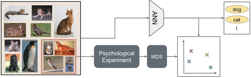
Generalizing Psychological Similarity Spaces to Unseen Stimuli                            3

2 Multidimensional Scaling

2.1 Obtaining Dissimilarity Ratings

In order to collect similarity ratings from human participants, several different tech-
niques can be used (Goldstone, 1994; Hout et al., 2013; Wickelmaier, 2003). They
are typically grouped into direct and indirect methods: In direct methods, partici-
pants are fully aware that they rate, sort, or classify different stimuli according to their
pairwise dissimilarities. Indirect methods on the other hand are based on secondary
empirical measurments such as confusion probabilities or reaction times.

    One of the classical direct techniques directly asks the participants for dissimilar-
ity ratings. In this approach, all possible pairs from a set of stimuli are presented to
participants (one pair at a time), and participants rate the dissimilarity of each pair
on a continuous or categorical scale. Another direct technique is based on sorting
tasks. For instance, participants might be asked to group a given set of stimuli into
piles of similar items. In this case, similarity is binary – either two items are sorted
into the same pile or not.
    Perceptual confusion tasks can be used as an indirect technique for obtaining
similarity ratings. For example, participants are asked to report as fast as possible
whether two displayed items are the same or different. In this case, confusion prob-
abilities and reaction times are measured in order to infer the underlying similarity
relation.

    Goldstone (1994) has argued that the classical approaches for collecting similarity
data are limited in various ways. Their biggest shortcoming is that explicitly testing
all N ·(N2 −1) stimulus pairs is quite time-consuming. An increasing number of stimuli
therefore leads to the need for very long experimental sessions, which might cause
fatigue effects. Moreover, in the course of such long sessions, participants might
switch to a different rating strategy after some time, making the collected data less
homogeneous.
    In order to make the data collection process more time-efficient, Goldstone (1994)
has proposed the “Spatial Arrangement Method” (SpAM). In this collection tech-
nique, multiple visual stimuli are displayed on a computer screen. In the beginning,
the arrangement of these stimuli is randomized. Participants are then asked to arrange
them via drag and drop in such a way that the distances between the stimuli are pro-
portional to their dissimilarities. Once participants are satisfied with their solution,
they can store the arrangement. The dissimilarity of two stimuli is then recorded
as their Euclidean distance in pixels. As N items can be displayed at once, each
single modification by the user updates N distance values at the same time which
makes this procedure quite efficient. Moreover, SpAM quite naturally incorporates
geometric constraints: If A and B are placed close together and C is placed far away
from A, then it cannot be very close to B.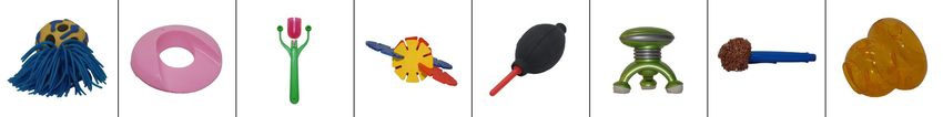
4                                                 Lucas Bechberger and Kai-Uwe Kühnberger

   As the dissimilarity information is recorded in the form of Euclidean distances,
one might assume that the dissimilarity ratings obtained through SpAM are ratio
scaled. This view is for instance held by Hout et al. (2014). However, as participants
are likely to make only a rough arrangement of the stimuli, this assumption might
be too strong in practice. One can argue that it is therefore safer to only assume an
ordinal scale. As far as we know, there have been no explicit investigations on this
subject. We will provide an analysis of this topic in Section 3.

2.2 The Algorithms

In this chapter, we follow the mathematical notation by Kruskal (1964a), who gave
the first thorough mathematical treatment of (nonmetric) multidimensional scaling.
   One can typically distinguish two types of MDS algorithms (Wickelmaier, 2003),
namely metric and nonmetric MDS. Metric MDS assumes that the dissimilarities
are interval or ratio scaled while nonmetric MDS only assumes an ordinal scale.
   Both variants of MDS can be formulated as an optimization problem involving the
pairwise dissimilarities δi j between stimuli and the Euclidean distances di j between
their corresponding points in the t-dimensional similarity space. More specifically,
MDS involves minimizing the so-called “stress” which measures to which extent the
spatial representation violates the information from the dissimilarity matrix:
                                       v
                                       u                       2
                                                           ˆ
                                       u
                                       u
                                       tÍ          d   −  d
                                           i< j     ij      ij
                              stress =      Í             2
                                                i< j di j

   The denominator in this equation serves as a normalization factor in order to
make stress invariant to the scale of the similarity space.
   In metric MDS, we use dˆi j = a · δi j to compute stress. This means that we look
for a configuration of points in the similarity space whose distances are a linear
transformation of the dissimilarities.
   In nonmetric MDS, on the other hand, the dˆi j are not obtained by a linear but by a
monotone transformation of the dissimilarities: Let us order the dissimilarities of the
stimuli in ascending order: δi1 j1 < δi2 j2 < δi3 j3 < . . . . The dˆi j are then obtained by
defining an analogous ascening order: dˆi1 j1 < dˆi2 j2 < dˆi3 j3 < . . . . Nonmetric MDS
therefore only tries to reflect the ordering of the dissimilarities in the distances while
metric MDS also tries to take into account their differences and ratios.

   There are different approaches towards optimizing the stress function, resulting in
different MDS algorithms. Kruskal’s original nonmetric MDS algorithm (Kruskal,
1964b) is based on gradient descent: In an interative procedure, the derivative of the
stress function with respect to the coordinates of the individual points is computed
and then used to make a small adjustment to these coordinates. Once the derivative
becomes close to zero, a minimum of the stress fuction has been found.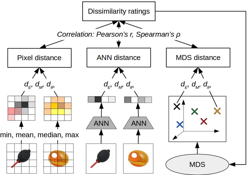
Generalizing Psychological Similarity Spaces to Unseen Stimuli                          5

    A more recent MDS algorithm by de Leeuw (1977) is called SMACOF (an
acronym of “Scaling by Majorizing a Complicated Function”). De Leeuw pointed
out that Kruskal’s gradient descent method has two major shortcomings: Firstly, if
the points for two stimuli coincide (i.e., xi = x j ), then the distance function of these
two points is not differentiable. Secondly, Kruskal was not able to give a proof of
convergence for his algorithm.
    In order to overcome these limitations, De Leeuw showed that minimizing the
stress function is equivalent to maximizing another function λ which depends on the
distances and dissimilarities. This function can be easily expressed by matrix multi-
plications of the configuration of points in the similarity space with two matrices. De
Leeuw proved that by iteratively multiplying the configuration with these matrices,
one can maximize λ and thus minimize stress. Moreover, one can prove that this
iterative procedure converges. SMACOF is computationally efficient and guarantees
a monotone convergence of stress (Borg and Groenen, 2005, Chapter 8).

    Picking the right number of dimensions t for the similaritiy space is not trivial.
Kruskal (1964a) proposes two approaches to address this problem:
    On the one hand, one can create a so-called “Scree” plot that shows the final
stress value for different values of t. If one can identify an “elbow” in this diagram
(i.e., a point after which the stress decreases much slower than before), this can point
towards a useful value of t.
    On the other hand, one can take a look at the interpretability of the generated
configurations. If the optimal configuration in a t-dimensional space has a sufficient
degree of interpretability and if the optimal configuration in a t + 1 dimensional
space does not add more structure, then a t-dimensional space might be sufficient.

3 Extracting Similarity Spaces from the NOUN Data Set

It is debatable whether metric or nonmetric MDS should be used with data collected
through SpAM. Nonmetric MDS makes less assumptions about the underlying mea-
surement scale and therefore seems to be the “safer” choice. If the dissimilarities
are however ratio scaled, then metric MDS might be able to harness these pieces
of information from the distance matrix as additional constraints. This might then
result in a semantic space of higher quality.

   In our study, we compare metric to nonmetric MDS on a data set obtained through
SpAM. If the dissimilarities obtained through SpAM are not ratio scaled, then the
main assumption of metric MDS is violated. We would then expect that nonmetric
MDS yields better solutions than metric MDS. If the dissimilarities obtained through
SpAM are however ratio scaled and if the differences and ratios of dissimilarities do
contain considerable amounts of additional information, then metric MDS should
have a clear advantage over nonmetric MDS.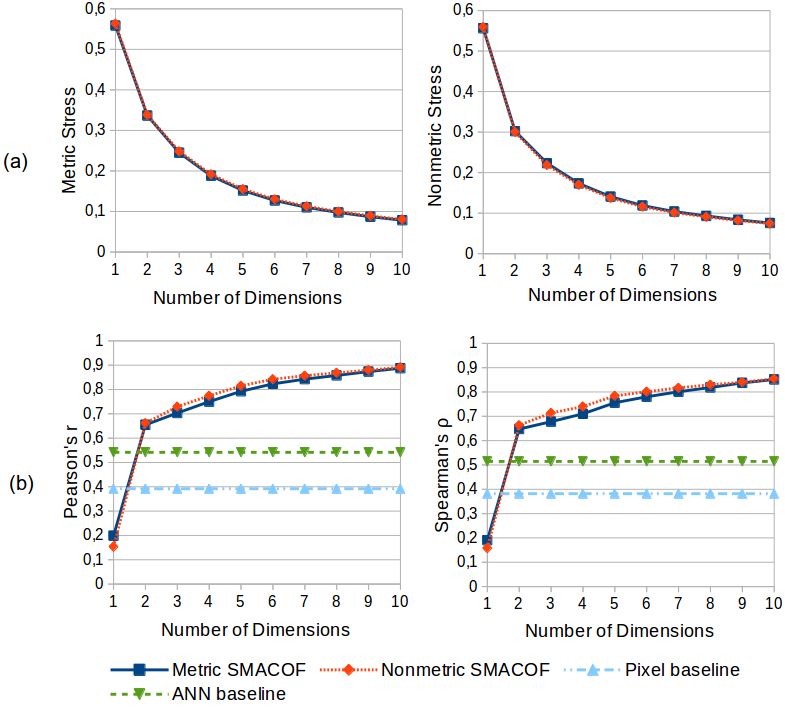
6                                                 Lucas Bechberger and Kai-Uwe Kühnberger

Fig. 1 Eight example stimuli from the NOUN data set (Horst and Hout, 2016).

   For our study, we used existing dissimilarity ratings reported for the Novel Object
and Unusual Name (NOUN) data set (Horst and Hout, 2016), a set of 64 images of
three-dimensional objects that are designed to be novel but also look naturalistic.
Figure 1 shows some example stimuli from this data set.

3.1 Evaluation Metrics

We used the stress0 function from R’s smacof package to compute both metric
and nonmetric stress. We expect stress to decrease as the number of dimensions
increases. If the data obtained through SpAM is ratio scaled, then we would expect
that metric MDS achieves better values on metric stress (and potentially also on
nonmetric stress) than nonmetric MDS. If the SpAM dissimilarities are not ratio
scaled, then metric MDS should not have any advantage over nonmetric MDS.

   Another possible way of judging the quality of an MDS solution is to look for
interpretable directions in the resulting space. However, Horst and Hout (2016) have
argued that for the novel stimuli in their data set there are no obvious directions that
one would expect. Without a list of candidate directions, an efficient and objective
evaluation based on interpretable directions is however hard to achieve. We therefore
did not pursue this way of evaluating similarity spaces.

   As an additional way of evaluation, we measured the correlation between the
distances in the MDS space and the dissimilarity scores from the psychological
study.
   Pearson’s r (Pearson, 1895) measures the linear correlation of two random vari-
ables by dividing their covariance by the product of their individual variances. Given
two vectors x and y (each containing N samples from the random variables X and Y ,
respectively), Pearson’s r can be estimated as follows, where x̄ and ȳ are the average
values of the two vectors:
                                    Ín
                                         (xi − x̄)(yi − ȳ)
                        rxy = qÍ i=1            qÍ
                                  n
                                      (x −    2     n             2
                                  i=1 i    x̄)      i=1 (yi − ȳ)

  Spearman’s ρ (Spearman, 1904) generalizes Pearson’s r by allowing also for
nonlinear monotone relationships between the two variables. It can be computed by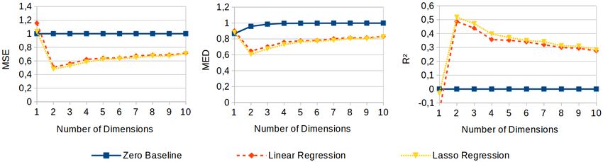
Generalizing Psychological Similarity Spaces to Unseen Stimuli                      7

replacing each observation xi and yi with its corresponding rank, i.e., its index in
a sorted list, and by then computing Pearson’s r on these ranks. By replacing the
actual values with their ranks, the numeric distances between the sample values lose
their importance – only the correct ordering of the samples remains important. Like
Pearson’s r, Spearman’s ρ is confined to the interval [-1, 1] with positive values
indicating a monotonically increasing relationship.
   Both MDS variants can be expected to find a configuration such that there is a
monotone relationship between the distances in the similarity space and the original
dissimilarity matrix. That is, smaller dissimilarites correspond to smaller distances
and larger dissimilarities correspond to larger distances. For Spearman’s ρ, we there-
fore do not expect any notable differences between metric and nonmetric MDS. For
metric MDS, we also expect there to be a linear relationship between dissimilarities
and distances. Therefore, if the dissimilarities obtained by SpAM are ratio scaled,
then metric MDS should give better results with respect to Pearson’s r than non-
metric MDS.

   A final way for evaluating the similarity spaces obtained by MDS is visual in-
spection: If a visualization of a given similarity space shows meaningful structures
and clusters, this indicates a high quality of the semantic space. We limit our visual
inspection to two-dimensional spaces.

3.2 Methods

In order to investigate the differences between metric and nonmetric MDS in the
context of SpAM, we used the SMACOF algorithm in its original implementation in
R’s smacof library.2 SMACOF can be used in both a metric and a nonmetric variant.
The underlying algorithm stays the same, only the definition of stress and thus the
optimization target differs. Both variants were explored in our study. We used 256
random starts with the maximum number of iterations per random start set to 1000.
The overall best result over these 256 random starts was kept as final result.
   For each of the two MDS variants, we constructed MDS spaces of different di-
mensionalities (ranging from one to ten dimensions). For each of these resulting
similarity spaces, we computed both its metric and its nonmetric stress.

   In order to analyze how much information about the dissimilarities can be readily
extracted from the images of the stimuli, we also introduced two baselines.
   For our first baseline, we used the similarity of downscaled images: For each
original image (with both a width and height of 300 pixels), we created lower-
resolution variants by aggregating all the pixels in a k × k block into a single pixel
(with k ∈ [2, 300]). We compared different aggregation functions, namely, minimum,

2 See https://cran.r-project.org/web/packages/smacof/smacof.pdf
8                                                       Lucas Bechberger and Kai-Uwe Kühnberger

Fig. 2 Illustration of our analysis setup: We measure the correlation between the dissimilarity
ratings and distances from three different sources: The pixels of downscaled images (left), activations
of an artificial neural network (middle) and similarity spaces obtained by MDS (right).

mean, median, and maximum. The pixels of the resulting downscaled image were
then interpreted as a point in a d 300     300
                                    k e × d k e dimensional space.
   For our second baseline, we extracted the activation vectors from the second-to-
last layer of the Inception-v3 network (Szegedy et al., 2016) for each of the images
from the NOUN data set. Each stimulus was thus represented by its corresponding
activation pattern. While the downscaled images represent surface level informa-
tion, the activation patterns of the neural network can be seen as more abstract
representation of the image.
   For each of the three representation variants (downscaled images, ANN activa-
tions, and points in an MDS-based similarity space), we computed three types of
distances between all pairs of stimuli: The Euclidean distance dE , the Manhattan
distance d M , and the negated inner product dI P . We only report results for the best
choice of the distance function. For each distance function, we used two variants: One
where all dimensions are weighted equally and another one where optimal weights
for the individual dimensions were estimated based on a non-negative least squares
regression in a five-fold cross validation (cf. Peterson et al. (2018) who followed a
similar procedure). For each of the resulting distance matrices, we compute the two
correlation coefficients with respect to the target dissimilarity ratings. We consider
only matrix entries above the diagonal as the matrices are symmetric and as all
entries on the diagonal are guaranteed to be zero. Our overall workflow is illustrated
in Figure 2.
Generalizing Psychological Similarity Spaces to Unseen Stimuli 9
Fig. 3 (a) Scree plots for both metric and nonmetric stress. (b) Correlation evaluation for the
different MDS solutions and the two baselines.
3.3 Results
Figure 3a shows the Scree plots of the two MDS variants for both metric and non-
metric stress. As one would expect, stress decreases with an increasing number of
dimensions: More dimensions help to represent the dissimilarity ratings more ac-
curately. Metric and nonmetric SMACOF yield almost identical performance with
respect to both metric and nonmetric stress. This suggests that interpreting the SpAM
dissimilarity ratings as ratio scaled is neither helpful nor harmful.
Figure 3b shows some line diagrams illustrating the results of the correlation
analysis for the MDS-based similarity spaces. For both baselines, the usage of
optimized weights considerably improved performance. As we can see, the ANN
baseline outperforms the pixel baseline with respect to both evalulation metrics,
indicating that raw pixel information is less useful in our scenario than the more
high-level features extracted by the ANN. For the pixel baseline, we observed that
the minimum aggregator yielded the best results.
We also observe in Figure 3b that the MDS solutions provide us with a better
reflection of the dissimilarity ratings than both pixel-based and ANN-based distances
if the similarity space has at least two dimensions. This comes as no surprise as the
MDS solutions are directly based on the dissimilarity ratings whereas both baselines10 Lucas Bechberger and Kai-Uwe Kühnberger
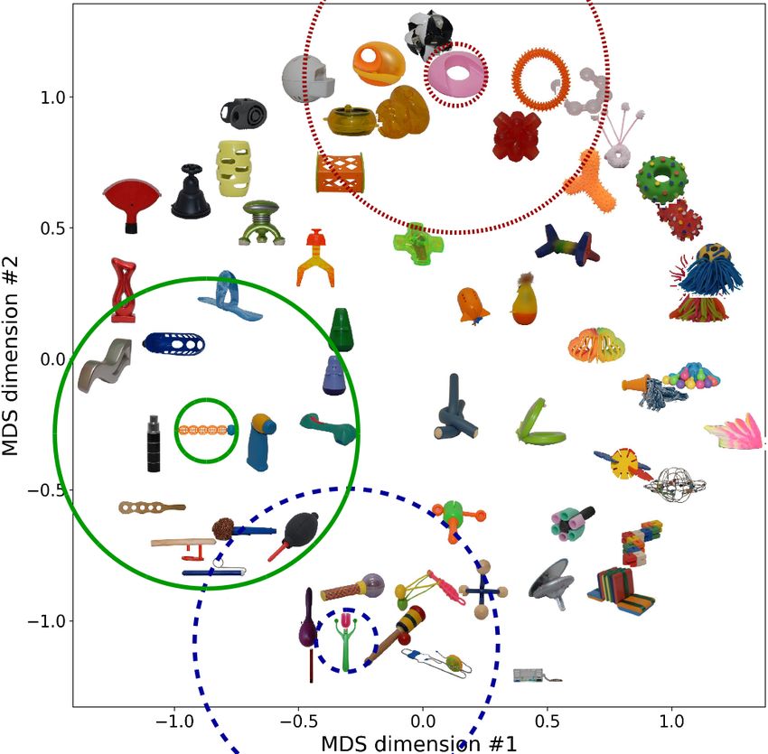
Fig. 4 Illustration of the two-dimensional spaces obtained by metric SMACOF (left) and nonmetric
SMACOF (right).
do not have access to the dissimilarity information. It therefore seems like our naive
image-based ways of defining dissimilarities are not sufficient.
With respect to the different MDS variants, also the correlation analysis confirms
our observations from the Scree plots: Metric and nonmetric SMACOF are almost
indistinguishable. This again supports the view that the assumption of ratio scaled
dissimilarity ratings is neither beneficial nor harmful for out data set. Moreover, we
find the tendency of improved performance with an increasing number of dimen-
sions. This again illustrates that MDS is able to fit more information into the space
if this space has a larger dimensionality.
Finally, let us look at the two-dimensional spaces generated by the different MDS
algorithms in order to get an intuitive feeling for their semantic structure. Figure 4
shows these spaces along with the local neighborhood of three selected items. These
neighborhoods illustrate that in both spaces stimuli are grouped in a meaningful way.
From our visual inspection, it seems that both MDS variants result in comparable
semantic spaces with a similar structure.
Overall, we did not find any systematic difference between metric and nonmetric
MDS on the given data set. It thus seems that the metric assumption is neither
beneficial nor harmful when trying to extract a similarity space. On the one hand, we
cannot conclude that the dissimilarites obtained through SpAM are not ratio scaled.
On the other hand, the additional information conveyed by differences and ratios of
dissimilarities does not seem to impact the overall results. We therefore advocate the
usage of nonmetric MDS due to the smaller amount of assumptions made about the
dissimilarity ratings.Generalizing Psychological Similarity Spaces to Unseen Stimuli 11
Fig. 5 Illustration of the proposed hybrid procedure: A subset of data is used to construct a
conceptual space via MDS. A neural network is then trained to map images into this similarity
space, aided by a secondary task (e.g., classification).
4 A Hybrid Approach
4.1 Our Proposal
Multidimensional scaling (MDS) is directly based on human similarity ratings and
leads therefore to conceptual spaces which can be considered psychologically valid.
The prohibitively large effort required to elicit such similarity ratings on a large
scale however confines this approach to a small set of fixed stimuli. We propose to
use machine learning methods in order to generalize the similarity spaces obtained
by MDS to unseen stimuli. More specifically, we propose to use MDS on human
similarity ratings to “initialize” the similarity space and artificial neural networks
(ANNs) to learn a mapping from stimuli into this similarity space.
In order to obtain a solution having both the psychological validity of MDS spaces
and the possibility to generalize to unseen inputs as typically observed for neural
networks, we propose the following hybrid approach, which is illustrated in Figure 5:
After having determined the domain of interest (e.g., the domain of animals), one
first needs to acquire a data set of stimuli from this domain. This data set should
cover a wide variety of stimuli and it should be large enough for applying machine
learning algorithms. Using the whole data set with potentially thousands of stimuli in
a psychological experiment is however unfeasible in practice. Therefore, a relatively
small, but still sufficiently representative subset of these stimuli needs to be selected
for the elicitation of human dissimilarity ratings. This subset of stimuli is then used in
a psychological experiment where dissimilarity judgments by humans are obtained,
using one of the techniques described in Section 2.1.
In the next step, one can apply MDS to the collected dissimilarity judgments
in order to extract a spatial representation of the underlying domain. As stated in
Section 2.2, one needs to manually select the desired number of dimensions – either
based on prior knowledge or by manually optimizing the trade-off between high
representational accuracy and a low number of dimensions. The resulting similarity12 Lucas Bechberger and Kai-Uwe Kühnberger
space should ideally be analyzed for meaningful structures and a high correlation of
inter-point distances to the original dissimilarity ratings.
Once this mapping from stimuli (e.g., images of animals) to points in a similarity
space has been established, we can use it in order to derive a ground truth for a ma-
chine learning problem: We can simply treat the stimulus-point mappings as labeled
training instances where the stimulus is identified with the input vector and the point
in the similarity space is used as its label. We can therefore set up a regression task
from the stimulus space to the similarity space.
Artificial neural networks (ANNs) have been shown to be powerful regressors
that are capable of discovering highly non-linear relationships between raw low-level
stimuli (such as images) and desired output variables. They are therefore a natural
choice for this task. ANNs are typically a very data-hungry machine learning method
– they need large amounts of training examples and many training iterations in order
to achieve good performance. However, the available number of stimulus-point pairs
in our proposed procedure is quite low for a machine learning problem – as argued
before, we can only look at a small number of stimuli in a psychological experiment.
We propose to resolve this dilemma not only through data augmentation, but also
by introducing an additional training objective (e.g., correctly classifying the given
images into their respective classes such as cat and dog). This additional training
objective can also be optimized on all the remaining stimuli from the data set that
have not been used in the psychological experiment. Using a secondary task with
additional training data constrains the network’s weights and can be seen as a form
of regularization: These additional constraints are expected to counteract overfitting
tendencies, i.e., tendencies to memorize all given mapping examples without being
able to generalize.
Figure 5 illustrates the secondary task of predicting the correct classes. This ap-
proach is only applicable if the data set contains class labels. If the network is forced
to learn a classification task, then it will likely develop an internal representation
where all members of the same class are represented in a similar way. The net-
work then “only” needs to learn a mapping from this internal representation (which
presumedly already encodes at least some aspects of a similarity relation between
stimuli) into the target similarity space.
Another secondary task consists in reconstructing the original images from a
low-dimensional internal representation, using the structure of an autoencoder. As
the computation of the reconstruction error does not need any class labels, this is
applicable also to unlabeled data sets, which are in general larger and easier obtain
than labeled data sets. The network needs to accurately reconstruct the given stimuli
while using only information from a small bottleneck layer. The small size of the
bottleneck layer creates an incentive to encode similar input stimuli in similar ways
such that the corresponding reconstructions are also similar to each other. Again,
this similarity relation learned from the overall data set might be useful for learning
the mapping into the similarity space. The autoencoder structure has the additional
advantage that one can use the decoder network to generate an image based on aGeneralizing Psychological Similarity Spaces to Unseen Stimuli 13
point in the conceptual space. This can be a useful tool for visualization and further
analysis.
One should be aware that there is a difference between perceptual and conceptual
similarity: Perceptual similarity focuses on the similarity of the raw stimuli, e.g.,
with respect to their shape, size, and color. Conceptual similarity on the other hand
takes place on a more abstract level and involves conceptual information such as
the typical usage of an object or typical locations where a given object might be
found. For instance, a violin and a piano are perceptually not very similar as they
have different sizes and shapes. Conceptually, they might be however quite similar
as they are both musical instruments that can be found in an orchestra.
While class labels can be assigned on both the perceptual (round vs. elongated)
and the conceptual level (musical instrument vs. fruit), the reconstruction ob-
jective always operates on the perceptual level. If the similarity data collected in
the psychological experiment is of perceputal nature, then both secondary tasks
seem promising. If we however target conceptual similarity, then the classification
objective seems to be the preferable choice.
4.2 Related Work
Peterson et al. (2017, 2018) have investigated whether the activation vectors of a
neural network can be used to predict human similarity ratings. They argue that this
can enable researchers to validate psychological theories on large data sets of real
world images.
In their study, they used six data sets containing 120 images (each 300 by 300
pixels) of one visual domain (namely, animals, automobiles, fruits, furniture, vegeta-
bles, and “various”). Peterson et al. conducted a psychological study which elicited
pairwise similarity ratings for all pairs of images using a Likert scale. When apply-
ing multidimensional scaling to the resulting dissimilarity matrix, they were able to
identify clear clusters in the resulting space (e.g., all birds being located in a similar
region of the animal space). Also when applying a hierarchical clustering algorithm
on the collected similarity data, a meaningful dendrogram emerged.
In order to extract similarity ratings from five different neural networks, they
computed for each image the activation in the second-to-last layer of the network.
Then for each pair of images, they defined their similarity as the inner product
(uT v = i=1 ui vi ) of these activation vectors. When applying MDS to the resulting
Ín
dissimilarity matrix, no meaningful clusters were observed. Also a hierarchical clus-
tering did not result in a meaningful dendrogram. When considering the correlation
between the dissimilarity ratings obtained from the neural networks and the human
dissimilarity matrix, they were able to achieve values of R2 between 0.19 and 0.58
(depending on the visual domain).
Peterson et al. found that their results considerably improved when using a
weighted version of the inner product ( i=1 wi ui vi ): Both the similarity space ob-
Ín14 Lucas Bechberger and Kai-Uwe Kühnberger tained by MDS and the dendrogram obtained by hierarchical clustering became more human-like. Moreover, the correlation between the predicted similarities and the human similarity ratings increased to values of R2 between 0.35 and 0.74. While the approach by Peterson et al. illustrates that there is a connection between the features learned by neural networks and human similarity ratings, it differs from our proposed approach in one important aspect: Their primary goal is to find a way to predict the similarity ratings directly. Our research on the other hand is focused on predicting points in the underlying similarity space. Sanders and Nosofsky (2018) have used a data set containing 360 pictures of rocks along with an eight-dimensional similarity space for a study which is quite similar in spirit to what we will present in Section 5. Their goal was to train an ensemble of convolutional neural networks for predicting the correct coordinates in the similarity space for each rock image from the data set. As the data set is considerably too small for training an ANN from scratch, they used a pre-trained network as a starting point. They removed the topmost layers and replaced them by untrained fully connected layers with an output of eight linear units, one per dimension of the similarity space. In order to increase the size of their data set, they applied data augmentation methods by flipping, rotating, cropping, stretching and shrinking the original images. Their results on the test set showed a value of R2 of 0.808, which means that over 80 percent of the variance was accounted for by the neural network. Moreover, an exemplar model on the space learned by the convolutional neural network was able to explain 98.9 percent of the variance seen in human categorization performance. The work by Sanders and Nosofsky is quite similar in spirit to our own approach: Like we, they train a neural network to learn the mapping between images and a similarity space extracted from human similarity ratings. They do so by resorting to a pretrained neural network and by using data augmentation techniques. While they use a data set of 360 images, we are limited to an even smaller data set containing only 64 images. This makes the machine learning problem even more challanging. Moreover, the data set used by Sanders and Nosofky is based on real objects, whereas our study investigates a data set of novel and unknown objects. Finally, while they confine themselves to a single target similarity space for their regression task, we investigate the influence of the target space on the overall results. 5 Machine Learning Experiments In order to validate whether our proposed approach is worth pursuing, we conducted a feasibility study based on the similarity spaces obtained for the NOUN data set in Section 3. Instead of training a neural network from scratch, we limit ourselved to a simple regression on top of a pre-trained image classification network. With the three experiments in our study, we address the following three research questions, respectively:
Generalizing Psychological Similarity Spaces to Unseen Stimuli                     15

 1. Can we learn a useful mapping from coloured images into a low-dimensional
    psychological similarity space from a small data set of novel images for which
    no background knowledge is available?
    Our prediction: The learned mapping is able to clearly beat a simple baseline.
    However, it does not reach the level of generalization observed in the study of
    Sanders and Nosofsky (2018) due to the smaller amount of data available.
 2. How does the MDS algorithm being used to construct the target similarity space
    influence the results?
    Our prediction: There is are no considerable differences between metric and
    nonmetric MDS.
 3. How does the size of the target similarity space (i.e., the number of dimensions)
    influence the machine learning results?
    Our prediction: Very small target spaces are not able to reflect the similarity
    ratings very well and do not contain much meaningful structure. Very large target
    spaces on the other hand increase the number of parameters in the model which
    makes overfitting more likely. By this reasoning, medium-sized target spaces
    should provide a good trade-off and therefore the best regression performance.

5.1 Methods

Please recall from Section 3 that the NOUN data base contains only 64 images with
an image size of 300 by 300 pixels. As this number of training examples is too low
for applying machine learning techniques, we augmented the data set by applying
random crops, a Gaussian blur, additive Gaussian noise, affine transformations (i.e.,
rotations, shears, translations, scaling), and by manipulating the image’s contrast
and brightness. These augmentation steps were executed in random order and with
randomized parameter settings. For each of the original 64 images, we created 1,000
augmented versions, resulting in a data set of 64,000 images in total. We assigned
the target coordinates of the original image to each of the 1,000 augmented versions.

   For our regression experiments, we used two different types of feature spaces:
The pixels of downscaled images and high-level activation vectors of a pre-trained
neural network.
   For the ANN-based features, we used the Inception-v3 network (Szegedy et al.,
2016). For each of the augmented images, we used the activations of the second-to-
last layer as a 2048-dimensional feature vector. Instead of training both the mapping
and the classification task simultaneously (as discussed in Section 4), we use an
already pre-trained network and augment it by an additional output layer.
   As a comparison to the ANN-based features, we used an approach similar to the
pixel baseline from Section 3.2: We downscaled each of the augmented images by
dividing it into equal-sized blocks and by computing the minimum (which has shown
the best correlation to the dissimilarity ratings in Secton 3.3) across all values in
each of these blocks as one entry of the feature vector. We used block sizes of 12 and
16 Lucas Bechberger and Kai-Uwe Kühnberger
24, resulting in feature vectors of size 1875 and 507, respectively (based on three
color channels for downscaled images of size 25 x 25 and 13 x 13, respectively). By
using these two pixel-based feature spaces we can analyze differences between low-
dimensional and high-dimensional feature spaces. As the high-dimensional feature
space is in the same order of magnitude as the ANN-based feature space, we can
also make a meaningful comparison betwen pixel-based features and ANN-based
features.
We compare our regression results to the zero baseline, which always predicts
the origin of the coordinate system. In preliminary experiments, it has shown to be
superior to any other simple baselines (such as e.g., drawing from a normal distribu-
tion estimated from the training targets). We do not expect this baseline to perform
well in our experiments, but it defines a lower performance bound for the regressors.
In our experiments, we limit ourselves to two simple off-the-shelf regressors,
namely a linear regression and a lasso regression. Let N be the number of data
points, t be the number of target dimensions, yd(i) the target value of data point i in
dimension d and fd(i) the prediction of the regressor for data point i in dimension d.
Both of our regressors make use of a simple linear model for each of the dimen-
sions in the target space:
ÕK
fd = w0(d) + wk(d) xk
k=1
Here, K is the number of features and x is the feature vector. In a linear least-squares
regression, the weights wk(d) of this model are estimated by minimizing the mean
squared error between the model’s predictions and the actual ground truth value:
N
1 Õ (i) 2
MSEd = yd − fd(i)
N i=1
As the number of features is quite high, even a linear regression needs to estimate
a large number of weights. In order to prevent overfitting, we also consider a lasso
regression which additionally incorporates the L1 norm of the weight matrix as
regularization term. It minimizes the following objective:
N K
1 Õ (i) 2 1 Õ (d)
yd − fd(i) + β · · w
N i=1 K k=1 k
The first part of this objective corresponds to the mean squared error of the linear
model’s predictions, while the second part corresponds to the overall size of the
weights. If the constant β is tuned correctly, this can prevent overfitting and thus
improve performance on the test set. In our experments, we investigated the following
values:Generalizing Psychological Similarity Spaces to Unseen Stimuli 17
β ∈ {0.0, 0.001, 0.002, 0.005, 0.01, 0.02, 0.05, 0.1, 0.2, 0.5, 1.0, 2.0, 5.0, 10.0}
Please note that β = 0 corresponds to an ordinary linear least-squares regression.
With our experiments, we would also like to investigate whether learning a map-
ping into a psychological similarity space is easier than learning a mapping into an
arbitrary space of the same dimensionality. In addition to the real regression targets
(which are the coordinates from the similarity space obtained by MDS), we created
another set of regression targets by randomly shuffling the assignment from images to
target points. We ensured that all augmented images created from the same original
image were still mapped onto the same target point. With this shuffling procedure,
we aimed to destroy any semantic structure inherent in the target space. We expect
that the regression works better for the original targets than for the shuffled targets.
In order to evaluate both the regressors and the baseline, we used three different
evaluation metrics.
• The mean squared error (MSE) sums over the average squared difference be-
tween the prediction and the ground truth for each output dimension.
t N
Õ 1 Õ (i) 2
MSE = · yd − fd(i)
d=1
N i=1
• The mean euclidean distance (MED) provides us with a way of quantifying
the average distance between the prediction and the target in the similarity space.
v
u
N t t
1 Õ Õ (i) 2
MED = · yd − fd(i)
N i=1 d=1
• The coefficient of determination R2 can be interpreted as the amount of vari-
ance in the targets that is explained by the regressor’s predictions.
S (d)
t
! N
21 Õ (d)
Õ 2
R = · 1 − residual
(d)
with Sresidual = yd(i) − fd(i)
t d=1 Stot i=1
al
N
Õ 2
(d)
and Stot al
= yd(i) − ȳ
i=1
We evaluated all regressors using an eight-fold cross validation approach, where
each fold contains all the augmented images generated from eight of the original
images. In each iteration, one of these folds was used as test set, whereas all other folds
were used as training set. We aggregated all predictions over these eight iterations
(ending up with exactly one prediction per data point) and computed the evaluation
metrics on this set of aggregated predictions.18 Lucas Bechberger and Kai-Uwe Kühnberger
Test Set Performance Degree of Overfitting
Regression Feature Space Targets β
MSE MED R2 MED MED R2
Baseline Any Any 1.0000 0.9962 0.0000 1.0000 1.0000 1.0000 –
ANN Correct 0.6153 0.7590 0.3701 36.5317 6.4187 2.6555 –
(2048) Shuffled 1.1804 1.0641 -0.1815 49.7003 7.5766 -5.3788 –
Pixel Correct 1.3172 1.0845 -0.3251 2.6191 1.6310 -1.5199 –
Linear
(1875) Shuffled 1.5915 1.2170 -0.5860 2.5953 1.6424 -0.6625 –
Pixel Correct 1.2073 1.0428 -0.2120 2.3360 1.5433 -2.2664 –
(507) Shuffled 1.5077 1.1880 -0.5032 2.3792 1.5735 -0.7302 –
ANN (2048) Correct 0.5711 0.7249 0.4172 20.8883 4.8409 2.3302 0.01
Lasso Pixel (1875) Correct 0.9183 0.9391 0.0788 1.1320 1.1371 2.3313 0.2, 0.5
Pixel (507) Correct 0.8946 0.9292 0.1015 1.1677 1.1251 2.2538 0.05, 0.1
Table 1 Performance of the different regressors for different feature spaces and correct vs. shuf-
fled targets on the four-dimensional space by Horst and Hout (2016). The best results for each
combination of column and regressor are highlighted in boldface.
5.2 Experiment 1: Comparing Feature Spaces and Regressors
In our first experiment, we want to test the following hypotheses:
1. The learned mapping is able to clearly beat the baseline. However, it does not
reach the level of generalization observed in the study of Sanders and Nosofsky
(2018) due to the smaller amount of data available.
2. A regression from the ANN-based features is more successful than a regression
from the pixel-based features.
3. As the similarity spaces created by MDS encode semantic similarity by geomet-
ric distance, we expect that learning the correct mapping generalizes better to
the test set than learning a shuffled mapping.
4. As the feature vectors are quite large, the linear regression has a large number
of weights to optimize, inviting overfitting. Regularization through the L1 loss
included in the lasso regressor can help to reduce overfitting.
5. For smaller feature vectors, we expect less overfitting tendencies than for larger
feature vectors. Therefore, less regularization should be needed to achieve opti-
mal performance.
Here, we limit ourselves to a single target space, namely the four-dimensional
similarity space obtained by Horst and Hout (2016) through metric MDS.
Table 1 shows the results obtained in our experiment, grouped by the regression
algorithm, feature space, and target mapping used. We have also reported the ob-
served degree of overfitting. It is calculated by dividing training set performance by
test set performance. Perfect generalization would result in an amount of overfitting
of one, whereas larger values represent the factor to which the regression is more
successful on the training set than on the test set. Let us for now only consider the
linear regression.Generalizing Psychological Similarity Spaces to Unseen Stimuli 19
We first focus on the results obtained on the ANN-based feature set. As we can
see, the linear regression is able to beat the baseline when trained on the correct
targets. The overall approach therefore seems to be sound. However, we see strong
overfitting tendencies, showing that there is still room for improvement. When trained
on the shuffled targets, the linear regression completely fails to generalize to the test
set. This shows that the correct mapping (having a semantic meaning) is easier to
learn than an unstructured mapping. In other words, the semantic structure of the
similarity space makes generalization possible.
Let us now consider the pixel-based feature spaces. For both of these spaces,
we observe that linear regression performs worse than the baseline. Moreover, we
can see that learning the shuffled mapping results in even poorer performance than
learning the correct mapping. Due to the overall poor performance, we do not
observe very strong overfitting tendencies. Finally, when comparing the two pixel-
based feature spaces, we observe that the linear regression tends to perform better
on the low-dimensional feature space than on the high-dimensional one. However,
these performance differences are relatively small.
Overall, ANN-based features seem to be much more useful for our mapping task
than the simple pixel-based features, confirming our observations from Section 3.
In order to further improve our results, we now varied the regularization factor β
of the lasso regressor for all feature spaces.
For the ANN-based feature space, we are able to achieve a slight but consistent
improvement by introducing a regularization term: Increasing β causes poorer per-
formance on the training set while yielding improvements on the test set. The best
results on the test set are achieved for β = 0.01. If β however becomes too large,
then performance on the test set starts to decrease again – for β = 0.2 we do not see
any improvements over the vanilla linear regression any more. For β ≥ 5, the lasso
regression collapses and performs worse than the baseline.
Although we are able to improve our performance slightly, the gap between
training set performance and test set performance still remains quite high. It seems
that the overfitting problem can be somewhat mitigated but not solved on our data
set with the introduction of a simple regularization term.
When comparing our best results to the ones obtained by Sanders and Nosofsky
(2018) who achieved values of R2 ≈ 0.8, we have to recognize that our approach
performs considerably worse with R2 ≈ 0.4. However, the much smaller number of
data points in our experiment makes our learning problem much harder than theirs.
Even though we use data augmentation, the small number of different targets might
put a hard limit on the quality of the results obtainable in this setting. Moreover,
Sanders and Nosofsky retrained the whole neural network in their experiments
whereas we limit ourselves to the features extracted by the pretrained network.
As we are nevertheless able to clearly beat our baselines, we take these results as
supporting the general approach.
For the pixel-based feature spaces we can also observe positive effects of regu-
larization. For the large space, the best results on the test set are achieved for larger
values of β ∈ {0.2, 0.5}. These results are however only slightly better than baseline20 Lucas Bechberger and Kai-Uwe Kühnberger
Test Set Performance Amount of Overfitting
Regressor Target Space β
MSE MED R2 MSE MED R2
Horst and Hout 1.0000 0.9962 0.0000 1.0000 1.0000 1.0000 –
Baseline Metric SMACOF 1.0000 0.9981 0.0000 1.0000 1.0000 1.0000 –
Nonmetric SMACOF 1.0000 0.9956 0.0000 1.0000 1.0000 1.0000 –
Horst and Hout 0.6153 0.7590 0.3701 36.5317 6.4187 2.6555 –
Linear Metric SMACOF 0.6334 0.7697 0.3599 36.2300 6.3909 2.7299 –
Nonmetric SMACOF 0.6225 0.7590 0.3565 36.3861 6.3749 2.7560 –
Horst and Hout 0.5711 0.7249 0.4172 20.8883 4.8409 2.3302 0.01
Lasso Metric SMACOF 0.6160 0.7513 0.3766 21.5633 3.7147 2.5789 0.01, 0.05
Nonmetric SMACOF 0.5834 0.7284 0.3969 11.9882 3.6440 2.3936 0.05
Table 2 Comparison of the results obtainable on four-dimensional spaces created by different MDS
algorithms. Best results in each column are highlighted for each of the regressors.
performance. For the small pixel-based feature space, the optimal value of β lies
in {0.05, 0.1}, leading again to a test set performance comparable to the baseline.
In case of the small pixel-based feature space, already relatively small degrees of
regularization (β ≥ 1) lead to a collapse of the model.
Comparing the regularization results on the three feature spaces, we can conclude
that regularization is indeed helpful, but only to a small degree. On the ANN-based
feature space, we still observe a large amount of overfitting, and performance on
the pixel-based feature spaces is still relatively close to the baseline. Looking at the
optimal values of β, it seems like the lower-dimensional pixel-based feature space
needs less regularization than its higher-dimensional counterpart. Presumably, this
is caused by the smaller possibility for overfitting in the lower-dimensional feature
space. Even though the larger pixel-based feature space and the ANN-based feature
space have a similar dimensionality, the pixel-based feature space requires a larger
degree of regularization for obtaining optimal performance, indicating that it is more
prone to overfitting than the ANN-based feature space.
5.3 Experiment 2: Comparing MDS Algorithms
After having analyzed the soundness of our approach in experiment 1, we com-
pare target spaces of the same dimensionality, but obtained from different MDS
algorithms. More specifically, we compare the results from experiment 1 to results
obtainable on the four-dimensional spaces created by both metric and nonmetric
SMACOF in Section 3. Table 2 shows the results obtained in our second experiment.
In a first step, we can compare the different target spaces by taking a look at the
behavior of the zero baseline in each of them. As we can see, the values for MSE
and R2 are identical for all of the different spaces. Only for the MED we can observe
some slight variations, which can be explained by the slightly different arrangements
of points in the different similarity spaces.Generalizing Psychological Similarity Spaces to Unseen Stimuli 21
As we can see from Table 2, the results for the linear regression on the different
target spaces are comparable. This adds further support to our results from Section
3: Also when considering the usage as target space for machine learning, metric
MDS does not seem to have any advantage over nonmetric MDS.
Also for the lasso regressor we observed similar effects for all of the target spaces:
A certain amount of regularization is helpful to improve test set performance, while
too much emphasis on the regularization term causes both training and test set
performance to collapse. Again, we still observe a large amount of overfitting even
after using regularization. Again, the results are comparable across the different
target spaces. However, the optimal performance on the space obtained with metric
SMACOF is consistently worse than the results obtained on the other two spaces. As
the space by Horst and Hout is however also based on metric MDS, we cannot use
this observation as an argument for nonmetric MDS.
5.4 Experiment 3: Comparing Target Spaces of Different Size
In our third and final experiment in this study, we vary the number of dimensions
in the target space. More specifically, we consider similarity spaces with one to ten
dimensions that have been created by nonmetric SMACOF.
Table 3 displays the results obtained in our third experiment and Figure 6 provides
a graphical illustration. When looking at the zero baseline, we observe that the mean
Euclidean distance tends to grow with an increasing number of dimensions, with an
asymptote of one. This indicates that in higher-dimensional spaces, the points seem
to lie closer to the surface of a unit hypershpere around the origin. For both MSE
and R2 we do not observe any differences between the target spaces.
Let us now look at the results of the linear regression. It seems that for all the
evaluation metrics, a two-dimensional target space yields the best result. With an
increasing number of dimensions in the target space, performance tends to decrease.
We can also observe that the amount of overfitting is optimal for a two-dimensional
space and tends to increase with an increasing number of dimensions. A notable
exception is the one-dimensional space which suffers strongly from overfitting and
whose performance with respect to all three evaluation metrics is clearly worse than
the zero baseline.
The optimal performance of a lasso regressor on the different target spaces when
trained on the ANN-based features yields similar results: For all target spaces we
made again the observation the regularization can help to improve performance but
that too much regularization decreases performance. Again, we can only counteract
a relatively small amount of the observed overfitting. As we can see in Table 3, again
a two-dimensional space yields the best results.
Taken together, the results of our third experiment show that a higher-dimensional
target space makes the regression problem more difficult, but that a one-dimensional
target space does not contain enough semantic structure for a successful mapping.22 Lucas Bechberger and Kai-Uwe Kühnberger
Test Set Performance Amount of Overfitting
Regressor t β
MSE MED R2 MSE MED R2
1 1.0000 0.8665 0.0000 1.0000 1.0000 1.0000 –
2 1.0000 0.9581 0.0000 1.0000 1.0000 1.0000 –
3 1.0000 0.9848 0.0000 1.0000 1.0000 1.0000 –
4 1.0000 0.9956 0.0000 1.0000 1.0000 1.0000 –
5 1.0000 0.9965 0.0000 1.0000 1.0000 1.0000 –
Baseline
6 1.0000 0.9973 0.0000 1.0000 1.0000 1.0000 –
7 1.0000 0.9978 0.0000 1.0000 1.0000 1.0000 –
8 1.0000 0.9980 0.0000 1.0000 1.0000 1.0000 –
9 1.0000 0.9982 0.0000 1.0000 1.0000 1.0000 –
10 1.0000 0.9984 0.0000 1.0000 1.0000 1.0000 –
1 1.1547 0.9012 -0.1547 50.7798 7.6907 -6.3153 –
2 0.5087 0.6468 0.4869 33.6837 6.1353 2.0226 –
3 0.5589 0.7022 0.4380 35.0878 6.2391 2.2465 –
4 0.6225 0.7590 0.3565 36.3861 6.3749 2.7560 –
5 0.6420 0.7770 0.3512 37.2875 6.4258 2.7977 –
Linear
6 0.6441 0.7800 0.3396 37.1193 6.3781 2.8929 –
7 0.6753 0.8026 0.3193 38.0741 6.4568 3.0760 –
8 0.6859 0.8127 0.2996 38.1881 6.4699 3.2767 –
9 0.6878 0.8138 0.2936 38.2118 6.4540 3.3441 –
10 0.7136 0.8299 0.2754 39.1195 6.5218 3.5637 –
1 1.0306 0.8826 -0.0306 1.0327 1.0206 -0.0667 5, 10
2 0.4808 0.6064 0.5174 21.1853 4.3094 1.8888 0.01, 0.02
3 0.5274 0.6740 0.4715 17.1673 4.3433 2.0556 0.02
4 0.5834 0.7284 0.3969 11.9882 3.6440 2.3936 0.05
5 0.6229 0.7627 0.3720 25.6519 5.3451 2.6223 0.005
Lasso
6 0.6333 0.7726 0.3498 30.5197 5.8073 2.7982 0.002
7 0.6489 0.7813 0.3418 16.5268 4.2493 2.8098 0.02
8 0.6729 0.8037 0.3117 30.6533 5.8197 3.1370 0.002
9 0.6721 0.8019 0.3092 20.4216 4.7331 3.1257 0.01
10 0.7080 0.8261 0.2810 34.6693 6.1649 3.4854 0.001
Table 3 Performance of the zero baseline, the linear regression, and the lasso regression on target
spaces of different dimensionality t derived with nonmetric SMACOF, along with the relative
amount of overfitting. Best values for each column are highlighted for each of the regressors.
It seems that a two-dimensional space is in our case the optimal trade-off. However,
even the performance of the optimal regressor on this space is far from satisfactory,
urging for further research.
6 Conclusions
The contributions of this paper are twofold:
In our first study, we investigated whether the dissimilarity ratings obtained
throught SpAM are ratio scaled by applying both metric MDS (which assumes
a ratio scale) and nonmetric MDS (which only assumes an ordinal scale). Both MDS
variants produced comparable results – it thus seems that assuming a ratio scale isYou can also read