Extraction of road boundary from MLS data using laser scanner ground trajectory
←
→
Page content transcription
If your browser does not render page correctly, please read the page content below
Open Geosciences 2021; 13: 690–704
Research Article
Lichun Sui, Jianfeng Zhu*, Mianqing Zhong*, Xue Wang, and Junmei Kang
Extraction of road boundary from MLS data using
laser scanner ground trajectory
https://doi.org/10.1515/geo-2020-0264
received September 12, 2020; accepted May 19, 2021
1 Introduction and related works
Abstract: Various means of extracting road boundary Mobile laser scanning (MLS) is an advancing technology
from mobile laser scanning data based on vehicle trajec- acquiring high-density object data more efficiently within
tories have been investigated. Independent of positioning detectable distances from moving platforms [1–5]. MLS
and navigation data, this study estimated the scanner has been widely applied in numerous fields including
ground track from the spatial distribution of the point urban planning and management [6,7], intelligent trans-
cloud as an indicator of road location. We defined a typical portation [8–11], and highways [12,13]. Extracting road
edge block consisting of multiple continuous upward fluc- boundary from MLS data is challenging for complex scene
tuating points by abrupt changes in elevation, upward environments [4,9] with huge data volumes [2,14], occlu-
slope, and road horizontal slope. Subsequently, such edge sion [4,13], and the heterogeneous, sparse, and noisy states
blocks were searched for on both sides of the estimated of point clouds [14].
track. A pseudo-mileage spacing map was constructed to To establish the topological relationship of point
reflect the variation in spacing between the track and edge clouds, studies often project three-dimensional (3D) point
blocks over distance, within which road boundary points clouds onto two-dimensional (2D) planes to form grid
were detected using a simple linear tracking model. images. Thus, a series of image processing techniques
Experimental results demonstrate that the ground trajectory such as feature extraction [1,15,16], image segmentation
of the extracted scanner forms a smooth and continuous [8,17,18], and mathematical morphology [12,19] can be
string just on the road; this can serve as the basis for
performed based on neighborhood pixels. For example,
defining edge block and road boundary tracking algorithms.
the elevation difference within a grid or adjacent pixels
The defined edge block has been experimentally verified as
is often used as a boundary indicator [16,18,20–24]. It is
highly accurate and strongly noise resistant, while the
more intuitive to distinguish raised edges from road cross-
boundary tracking algorithm is simple, fast, and indepen-
sections [3,23,25], while vehicle trajectories provide the
dent of the road boundary model used. The correct detec-
direction of projection for edge generation. Xia et al. iden-
tion rate of the road boundary in two experimental data is
tified holes, detected break-lines from elevation image
more than 99.2%.
generated by point cloud, and matched patches along
Keywords: edge block, scanner ground track, pseudo- road for holes [26]. Constructing a 3D raster map with a
mileage spacing map, boundary tracking unit volume called voxel (volume pixel) [5,8,27] is the
other useful tool to simplify high-density point clouds.
For example, a greater density gradient in more than one
direction implies the existence of a road edge in ref. [5].
Considering the uneven density of raw data, Lin et al.
* Corresponding author: Jianfeng Zhu, College of Geological
generated super-voxels with adaptive resolution to pre-
Engineering and Geomatics, Chang’an University, Xi’an, Shaanxi
710054, China; Jiangxi College of Applied Technology, Ganzhou
serve edges with smaller segmentation error [27]. Sha
341000, China, e-mail: 2015026023@chd.edu.cn et al. further improved Lin’s method using geometric infor-
* Corresponding author: Mianqing Zhong, Faculty of Geomatics, mation to cluster the points when merging the point label
Lanzhou Jiaotong University, Lanzhou 730070, China, into its neighbor representative points [28]. Xu et al. clas-
e-mail: emmazho@mail.lzjtu.cn
sified point clouds using trend features of super voxels
Lichun Sui, Junmei Kang: College of Geological Engineering and
Geomatics, Chang’an University, Xi’an, Shaanxi 710054, China
[29].Despite its simplicity and convenience, converting
Xue Wang: College of Resources Environment and History Culture, point clouds into voxels may cause information loss and,
Xianyang Normal University, Xianyang, 712025, China consequently, reduces the accuracy [5].
Open Access. © 2021 Lichun Sui et al., published by De Gruyter. This work is licensed under the Creative Commons Attribution 4.0
International License.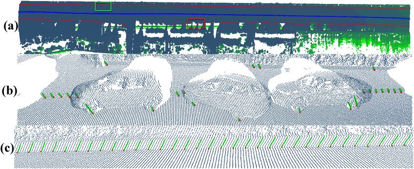
Extraction of road boundary from MLS data using laser scanner ground trajectory 691
On the contrary, extracting boundary directly from gathered clusters composed of many single points with
raw point clouds has gained increasing attention from large elevation gradients. As another contribution of this
point clouds experts. In this regard, k-dimensional (KD) study, multiple points of continuous upward fluctuation
trees [2,14,30] have been widely used to accelerate the are combined as a whole edge block without considera-
nearest neighbor search in data organization. Numerous tion of edge height.
methods based on scan lines that use the original record In addition, boundary points are distributed near
order have been developed for road boundary extraction. straight lines over a short distance [11]. Most road boundary
A scan line was divided into several segments in ref. vectorization is achieved by fitting straight lines to candi-
[2,20,31]. In addition, road segments were detected by date edge points [18,20], which adapts for straight-line or
line-based region growth and then fitted into straight large-radius mildly curved edges. However, setting curve
lines [8] or polynomial curves [15,17,32] have detected boundaries requires prior knowledge to define an appro-
boundary points using moving window operators on a priate fitting model. Based on the approximate equidistant
scan line or adjacent lines based on abrupt changes in relationship between the road edge and scanner trajectory,
elevation, point density, surface roughness [13], and the this study transforms the process of edge point tracking
angles formed by three consecutive points [21,33]. In most onto a pseudo-mileage spacing map, to which a linear
cases, the window size was fixed manually, and multiple model can be applied.
thresholds were defined from experience and adjusted fre- The remainder of this paper is organized as follows.
quently to accommodate distinct point cloud distributions. Section 2 details the proposed method. Section 3 presents
In these methods, candidate boundary points are and discusses the experimental results. Section 4 con-
usually extracted from segments or scan lines. The final cludes the paper.
boundary is determined via clustering, fitting, or boundary
tracking algorithms. Continuous closed polygons is
extracted in ref. [10] as a road boundary. Active contour
models were applied in ref. [6] to fix the optimal road 2 Methodology
boundary on projected 2D raster images of elevation,
reflectance, and pulse width. A discrete Kalman filter In this study, we propose a three-part method to quickly
[11,16] and α-shape [3,4,8] algorithms are often adopted extract road boundaries from MLS data based on the
to identify and track boundary points. To reduce errors scanner ground track. First, the scanner track is estimated
in tracking, multiple constraints are imposed to achieve from raw data using point density and slope. Then, edge
desired edge clusters, e.g., the distance between adjacent blocks composed of several continuously upward fluctuating
points, direction of historical boundary formed by pre- points are searched from both outer sides of the estimated
viously identified points [16], length constraints [1], and tracks. Finally, the spacing between the scanner trajectory
collinearity conditions of adjacent segments [15]. and extracted edge blocks is depicted in a pseudo-spacing
Although plenty of algorithms have been proposed mileage map to describe trends in spacing over distance tra-
for road boundary extraction from MLS data, there is a need veled. A simple linear model is deduced based on the proxi-
for a framework to efficiently extract the road boundary. mity and collinearity of boundary feature points in the map
In majority methods, vehicle trajectories have been used as to quickly detect and track boundary points. Figure 1 presents
a reference to locate the road boundary [3,6,20,34,35]. a simple flow chart of the proposed method.
Thanks to the road design parameters, unnecessary data
located far from the road can be easily filtered out
[9,17,18,21,36]. In addition, huge point clouds can be parti-
tioned into several segments [8,37,38] or cross-sectional 2.1 Estimation of laser scanner ground tracks
profiles [3,17,23,39] along the trajectory direction. However,
trajectory data may not be packaged in the original “.las” This study estimated scanner ground tracks based on
files. Therefore, instead of using external data, this study point density and slope in the three steps.
estimates the scanner ground trajectory directly from raw
point clouds, which is one of the key contributions of the
paper. 2.1.1 Extraction of road feature areas
Moreover, the routine height of curb stones is often
used to extract edges that are highly uniform in height As scan lines are perpendicular to vehicle trajectory, the
[20,24]. Candidate edge points are often detected as scanner ground trajectory is located at the densest part of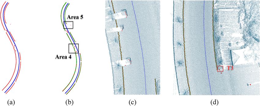
692 Lichun Sui et al.
Searching outwards
Detection of road
Raw Estimation of from the track for edge Road
boundaries in a
MLS the scanner blocks with several boundary
pseudo-mileage
data ground track continuously points
spacing map
fluctuating points
Figure 1: Flowchart of the proposed road boundary extraction method.
the point cloud with a slight slope [40]. Point density ( JS) distributed) swings left and right, which is not consistent
and slope ( Jn) are calculated using the following equations: with the driving rules. Therefore, a refining process is
1 necessary.
JSi = (Xi + k − Xi − k )2 + (Yi + k − Yi − k )2 + (Zi + k − Zi − k )2 , (1)
2k
∣Zi + 2 − Zi − 2∣
Jni = , (2) 2.1.3 Refinement of the estimated scanner ground
(Xi + 2 − Xi − 2)2 + (Yi + 2 − Yi − 2)2
trajectory
where 2k is the number of points counted in the neigh-
borhood (at least 20, to weaken the effect of spacing var- In Figure 2, colored strips indicate the road feature area
iation because of missing points); and Jni is formed TYF divided by time interval Δt, in which CG points (in
between the second point in front and second point red) swing as the point distribution varies when the
behind the i-th point to reduce the impact of noise and vehicle travels forward. To further refine CGi, we fitted
small fluctuations. Then those points for which TY = {P them to an isochromatic series based on T. The CG points
( JSi < median (JS) & Jni < 10°)} can be taken as the road are first returned to the original point data based on the
feature area. nearest neighbor principle (Euclidean distance). Then,
the corresponding scan lines number to the CG points
are detected. A test region of scan line frequency is con-
2.1.2 Obtaining rough scanner tracks structed between CGi and CGi−1 shown in black rectangle
in Figure 3.
Points high above a road with low slope may be extracted The test region is several times wider than the average
to TY because of environmental complexity. To remove point spacing and longer than the CG point spans. The
them, we segmented TY by time interval Δt, based on GPS value of T in test region has slightly change in points
time T. Let m be the number of segments after TY is 1–4, 5–8, and 9–11, while sharp time difference occurs at
segmented. Elevation is analyzed for each segment TYi, points 4–5 and 8–9. The sharp difference indicates the
where TYi = {TY((i −1) · Δt < Ti < i · Δt)}. Those points with approximate interval time between adjacent scan lines.
the most concentrated elevation distribution in TYi are Let it be tL. Then the scan line number CGi belongs to
retained and marked as the i-th road feature area TYFi, can be derived by:
TYFi = {TYi (ZP − ΔZ < Zi < ZP + ΔZ)}, where ZP represents
TCG − T1 1
the peak value in elevation histogram of TYFi and ΔZ SNli = i + , (3)
(0.2 m is recommended) is the allowable elevation toler- tL 2
ance. Rough scanner tracks CG (red points in Figure 2) are where the variable SNli denotes the sequence number of
obtained by averaging the coordinates of all points in the scanline CGi belongs, take the scan line of the first
each TYF, giving CGi = TYFi(X , Y , Z ). point of data set P as line 1.
In Figure 2, the rough estimated trajectory (centers All CGi points from multiple measurements of laser
of gravity of the high point-density areas horizontally foot points corresponding to the same scanning angle,
Figure 2: The rough estimated scanner ground tracks.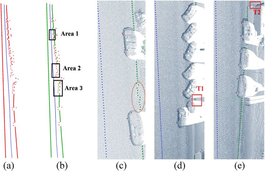
Extraction of road boundary from MLS data using laser scanner ground trajectory 693
illustrates the process of building edge blocks in four
consecutive steps.
As can be seen from this figure, in the first step, a
moving window is created to detect upward fluctuating
points (small squares in cyan in Figure 4) by height
differences. Window size is expressed as the number
of points contained within the window. The half
Figure 3: Test region to obtain the scan lines CGi belongs to. width (BMWi) of the window can be determined by
BMWi = ⌈Ch / (Jsi ⋅ sin θ)⌉, where Ch and θ denote the
minimum height (0.08 m) and minimum slope (30°) of
and their time T should meet the isochromatic sequence the boundary to be detected, respectively. The default
shown in equation (4). values of these parameters are considered according to
TCGi = t1 + (SNli − 1)⋅ td, (4) regulations on exposure height of curb stones in Chinese
city streets. In addition, window width varies with Jsi ; the
where t1 and td represent the reliable estimate of acquisi- larger the window, the fewer points it contains. The ele-
tion time of the refined ground track points on the first vation difference Hdiffi before and after the center point of
scan line, and the elapsed time of each scan line, respec- the window is calculated as:
tively. The point whose acquisition time closest to the
i + BMWi i−1
refined TCGi is taken as the estimated vehicle tracks which Hdiffi = ∑ Zj − ∑ Zj . (5)
is expressed as NPHi. i+1 i − BMWi
The point at which Hdiffi ≥ Ch is the upward point. We
only detected boundaries in the forward direction, that is,
2.2 Composition of edge blocks di + BMWi − di − BMWi > ε , where di + BMWi , di − BMWi denote the
distances of the last and the first point in the window
The raised curb is often detected as quantitative and dis- from NPHi. Tolerant ε is set to −0.1 m (to allow return of
crete candidate boundary points. This study combines 0.1 m). The search length in Figure 4 is set to 15 m,
continuous fluctuating points into edge blocks by according to conventional road design width. Two point
searching forward and backward from NPHi. Figure 4 sets A1 and A2 are formed by forward and backward
Figure 4: The process of composition of edge blocks.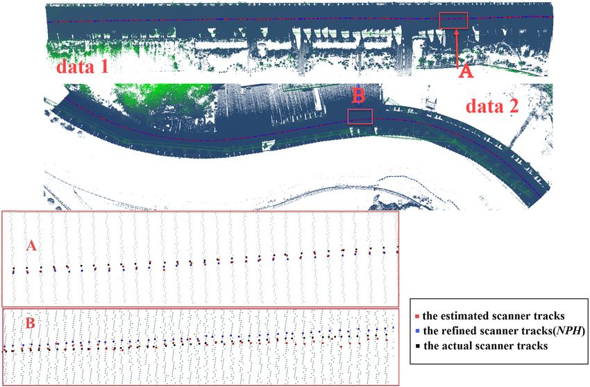
694 Lichun Sui et al.
searches from NPHi in opposite directions. In the fol- 2.3 Boundary tracking
lowing steps, forward search from A1 is taken as an
example. Frequent lane switching is not allowed during scanning,
The second step is to filter points by slope. We only which limits fluctuations in spacing between the road
consider the slope between central point i of the window boundary and the scanner’s ground track. This relation-
and the next point i + 1, which is given by: ship is reflected in a pseudo-mileage spacing map in
Zi + 1 − Zi Figure 5, in which NPHi points are represented as red
Slopei = . (6) circles. Blue and white rectangles denote the starting
(Xi + 1 − Xi)2 + (Yi + 1 − Yi )2
point of each block and generated candidate edge feature
Points with Slopei < tan(θ) are removed from the points, respectively. The gray line shows the scan lines
data. It is possible to have one or two continuous upward located at NPHi. There may be more than one edge block
points that may not be near the road boundary. However, extracted from NPHi. However, the first block in each
if continuous multiple points fluctuate upwards, they scan line is highly likely to belong to the roadside when
are more likely to belong to a boundary. We combined the road surface is relatively smooth. Points on the map
continuous upward fluctuation points into blocks in the are named candidate boundary feature points, corre-
third step. The consecutive number Bni must satisfy sponding to (∑1i Li , BSDij) of each boundary point, where
Bni ≥ max (⌊ηCh / J si ⌋ , 1), where η is the correction coef- Li is the Euclidean distance between adjacent NPHi. There
ficient determined by the ratio of the interquartile range are three processes to present the boundary tracking
to the total range of adjacent point spacing among 10 algorithm.
neighborhood points. The value of η depends on the Process 1: Extracting the initial feature segment of
rate of missing points; a value in the range of 0.7–1 is the road boundary
recommended. In most cases, yi varies little in a certain range of Δx.
In the last step, the elevation of NPHi, extracted in However, there is always a segment from the map longer
Section 2.1.3, is used to remove blocks whose starting than 5 m that accords with a robust linear regression
points are higher than the road surface.The filter is given model of 95% confidence. These segments are found in
in equation (7) and shown in Figure 4 with cyan shadows. the dataset composed of the first block of each scan line
Let (Xi, Yi, Zi) represent the position of NPHi and (BSXj, and are labeled the initial road boundary feature seg-
BSYj, BSZj) denote the coordinates of the start points ments (red line in Figure 6). Inside points satisfying
of the j-th block located on the NPHi scan line. The regression conditions are identified as boundary feature
threshold value of Zth is taken from the greater of the points, and end points at both sides are identified as the
two values of 0.1 m and 3% of the span according to last identification points (red points in Figure 6).
the horizontal slope of the road (generally 1.5–2%). In Figure 6, the initial feature segment of the road
∣BSZj − Zi∣ < Zth boundary is approximately in a straight line. We use this
(7) line as the direction to establish a possible area con-
Zth = max{0.1, 3% (BSXj − Xi)2 + (BSYj − Yi )2 }. taining nearby boundary feature points at the end of
the last identified feature points. The vertex angle of
As shown in Figure 4, the blue and green points are
the first and rest points of blocks, respectively. After mul-
tiple constraints, there are few edge blocks on an NPHi
scan line. If no edge blocks remain, the boundary point
corresponding to NPHi is labeled as null. Otherwise, fea-
ture information of discovered blocks, including BSDij ,
spacing from the starting point of the j-th block to PGi,
and BHij, the elevation difference in the block is extracted
for the boundary tracking process. These features are
calculated as:
BSDij = (BSXj − Xi)2 + (BSYj − Yi )2 + (BSZj − Zi)2
(8)
BHij = BEZj − BSZj ,
where BEZj represents the elevation of the last point in
the block. Figure 5: The pseudo-mileage spacing map.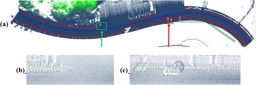
Extraction of road boundary from MLS data using laser scanner ground trajectory 695
road boundary. Then, the prediction yi+1 = yi improves
tracking speed.
Process 3: Tracking boundary feature points using a
hunting zone
We tracked boundary feature points using a hunting
zone (black in Figure 6) controlled by a fan-shaped center
angle α. As shown in Figure 6, α is opened along the
predicted direction, the vertex of which refers to the
Figure 6: Hunting zones derived by Δx and α. last recognized boundary feature point (the last green
point). We recommend an empirical model of α expressed
as α = (a exp(−bΔx)) + c, where, a, b, and c are constant
coefficients controlling the radian-unit fan-shaped angle.
the possible area changes with the distance (x) from the
The recommended values of (0.86, 0.76, 0.12) cause α to
vertex (the last identified points), whose size is deter-
decrease with the passing of Δx . In practice, the search
mined from Process 2.
area is converted into a hunting zone parallel to the
Process 2: Predicting the possible location of the next
y-axis direction and is deduced as follows:
boundary feature point
The vehicle keeps moving in its original direction R = 0.2 Δx ≤ 0.25 m
because of inertia. We first evaluated the separation of
α
()
2 tan 2 ⋅ Δx (10)
the vehicle from the road boundary based on the tail of R = 0.25 m < Δx < 15 m,
cos ψ
recognized edge feature points (not less than 3 m) where
Δy = ymax − ymin. If Δyr ≤ yth, where yth is a set threshold, where [yi + 1−R,yi + 1 + R] constitutes the hunting zone. If the
then the vehicle runs parallel to the road boundary hunting zone does not include a point where x = xi+1, then
and the possible location of the next boundary feature the search continues for x = xi+2. If multiple points are
point is close to the last recognized yi. Otherwise, the found in the hunting zone, the point with the smallest
separation of vehicle from road boundary is represented angle to the search direction is selected. However, as
as a regressed linear model. Then, yi+1 of the next boundary the distance between the current point and the final
feature point at xi+1 can be predicted as: identified boundary feature point (the last green point)
yi + 1 = yi Δyr ≤ yth increases, the reliability of tracking deteriorates. We
(9) set a maximum search length SLth of 15 m. Exceeding
yi + 1 = kl xi + 1 + kb Δyr > yth,
this length, the forward search process is interrupted
where y = klx + kb represents the regressed straight line and tracing in Processes 1–3 is re-implemented from
derived from the tail of the recognized boundary feature the last identified boundary feature point. Figure 7 illus-
points. Let ψ be the angle of the regressed line from the trates the segmentation of feature points in the tracking
positive x-axis, then ki = tan(ψ). The threshold yth is set at process.
0.25 m, giving a maximum deviation of 5° from the road The red line on the left side of Figure 7 is the initial
edge. It is common for vehicles to travel parallel to the edge feature segment recognized for the first time. It
Figure 7: Data segmentation in tracking process.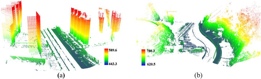
696 Lichun Sui et al.
divides dataset B into two segments B2 and B1, both of
which contain red line segments. Starting from the end
points (in red), the two sides are tracked in opposite
directions. The identified edge feature points tracked in
opposite directions are marked in green. If no point is
marked in SLth from the last identified point, the data
are disconnected. Beginning with the last green identified
point, a new search dataset B3 is constructed, on which
Processes 1–3 are executed again. The initial boundary
feature segment (red line on the right side of Figure 7) is
found for the second time. B3 is divided into B4 and B5
segments for forward and backward search, respectively.
Note that the overlapping search area B6 undergoes a
bidirectional search, forward search in the first dataset
Figure 8: Span cube based on two adjacent edge points. (a)–(c)
B1 and reverse search in B5. This can reduce the prob-
represent the search cube in axonometric, top, and side view,
ability of missing boundary points. Provided that the
respectively; (d) illustrates the length of the span cube.
recording order of data points in B2 and B5 is reversed,
the same search steps as those in B1 and B3 can be used.
boundary point i and the next point i + 1, respectively. φi
is the deviation angle formed by the line direction
obtained by least squares linear regression from five
2.4 Post-processing points before and after point i . When Con = 1, the point
i is connected to the next point; if not, points are not
Once the connection relations of the extracted boundary connected.
points on the scan line are determined, a rough vector-
ized boundary can be quickly obtained. The selection of
boundary mathematical models and the extraction of all
point clouds in the road are not addressed in this paper.
3 Results
The following sections focus on determining the connec-
tion between adjacent boundary points.
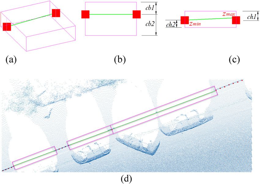
Length density Ld (m−1) of two boundary points is 3.1 Data
defined as the ratio of the number of points in their span-
ning region to their distance. Figure 8 illustrates the span Experimental data were collected with the SSW-IV vehicle
cube based on two adjacent points. In this figure, the red laser modeling and measurement system developed by
points are extracted edge points and the green lines con- the Chinese Academy of Surveying and Mapping. The
nect two adjacent boundary points, cb1, cb2 (set at 0.2 and laser scanner is located at the rear of the vehicle on
0.1) depict the searching width in the direction of heading the right and the scanning plane is perpendicular to the
or departing from the road, and ch1, ch2 in Figure 8(c) direction of travel. Within seconds, five million measure-
indicate the height range of the cube, where ch1 is higher ments and 100 scan lines are collected in a typical mea-
than the tallest point and ch2 lower than the lowest point surement range of 1–500 m with an angular accuracy of
(both set at 0.1). The connector Con describes the connec- 0.1 milliradians. Traveling at a speed of 30 km/h resulted
tion between adjacent boundary points as: in average spacing of 8 cm between adjacent scan lines,
and 0.6 cm between two adjacent points right below the
Con = 1 si − i + 1 ≤ 2 m vehicle. In addition, the scan angle information is not
1
Con = 1 Ld < &2 m < &si − i + 1 ≤ 20 m&φi < 10° , (11) included in the original .las file.
5A s
Con = 0 other The datasets shown in Figure 1 include two types of
road edge line: straight lines and curves. Two types of
where As and si − i + 1 refer to the average point spacing of curbstones are featured, with right angle and S-shaped
raw data and the Euclidean distance between the current cross-sections. Dataset 1 (185.4 MB, 5.7 million points,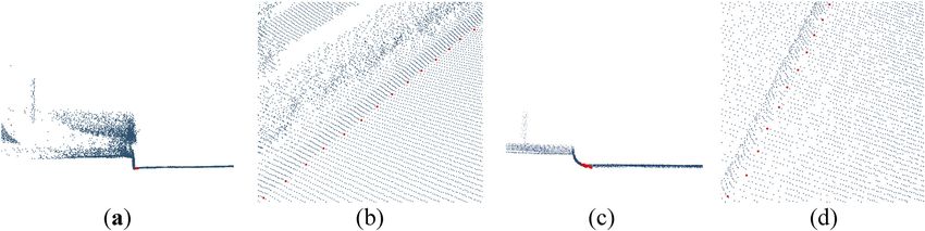
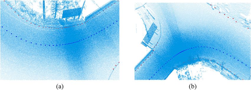
Extraction of road boundary from MLS data using laser scanner ground trajectory 697 Figure 9: The test area rendered by elevation in (a) Dataset 1 and (b) Dataset 2. 308 m long) displayed in Figure 9(a) is located in an 3.2 Estimation of laser scanner ground urban area with multiple road lanes, high-rise buildings, tracks trees, a green belt, poles, and wires. One side of the road edge is a straight line, and the other consists of broken The algorithm was performed on three sample datasets. lines with different tilt angles. Dataset 2 (279.4 MB, 4.8 The ground track of the scanner was estimated from two million points, 300 m long) depicted in Figure 9(b) lies on datasets at time intervals of 0.05 s, with an average dis- a winding highway with towering mountains on one side tance of 0.4–0.6 m. Figure 10 illustrates the differences and low-lying valleys on the other; it is surrounded by between the two estimated scanner ground tracks and several trees, sidewalks, fences, and electric facilities. the actual scanner position (black points). Red and blue With S-shaped cross-sectional roadside stones on both points indicate the horizontal position of NPH before and sides, the edges curve with changing radii. after refinement, respectively. As shown in Figure 10, Figure 10: Comparison of estimated scanner ground tracks with the real scanner position.
698 Lichun Sui et al.
points lie near the location of the vehicle in the road, rough scanner tracks, and consequently, ensure the accu-
and red dots are mixed with blue. After refinement, the racy of the trajectory estimation algorithm.
estimated scanner trajectory (formed by blue points)
is smoother. The results show that the deviation of
NPH (blue points) from the true value is not affected by
road curvature, but only to the roughness of the road 3.3 Extraction of edge blocks
surface. To verify the precision and accuracy of NPH,
we compared horizontal deviation from NPH to the actual Only boundary points on the scan line of estimated tracks
scanner location. Actual location of the scanner is were extracted. Compared to extracting on all scanning
acquired at a frequency several times that of NPH. We lines, the number of sampling boundary points is reduced
extracted scanner position data with the closest data and processing efficiency is improved. Table 1 shows the
acquisition time T. integrity and the noise of the edge blocks extracted from
The result shows that the deviation from the roughly two datasets.
estimated scanner ground tracks of Dataset 1 (such as The extracted edge blocks in Dataset 1 are shown in
Area A in Figure 10) to the actual trajectory is relatively Figure 11. The red points represent the starting point of
similar in each scanning line, while the estimated tracks edge blocks, and the green are other points contained in
of the Dataset 2 (gravity centers of high-density areas) the block. Left of the road, 832 ground track points (blue)
swinging around the actual ones. This phenomenon may correspond to 832 edge blocks (red) arranged neatly
be because of the greater roughness of the road surface of along the roadside in Figure 11(c). Locating the test
the Dataset 2, especially on the right side of Area B in area in a clean urban area with no obstructions on this
Figure 10. However, the refined algorithm redistributes side may be the main reason for this result. On the right,
the estimated deviation from each scan line so that the many vehicles are parked on the roadside, scattering and
refined scanner trajectory is very close to the actual one. fragmenting the extracted edge blocks. As Table 1 shows,
In fact, the more scan lines involved in the refinement, most noisy points were caused by vehicle occlusion in the
the more stable and accurate the refined tracks are. road; outside the road, noise is rare. Of the 813 edge
The estimated NPH shows strong uniformity with blocks extracted on the right side of the road, only seven
the actual scanner location, with a maximum value of points correspond to three edge blocks; the rest corre-
14.3 cm, mean deviation 2.1 cm and standard deviation spond to two at most. At the end of the green belt, two
1.3 cm. For the proposed boundary tracing algorithm, low edge blocks were not extracted.
the minimum width of the buffer is 40 cm, which is five Figure 12 demonstrates the extraction of edge blocks
times larger than the horizontal difference of the esti- in Dataset 2, which encountered the same vehicle occlu-
mated points. Thus, NPH can be used for boundary sion as Dataset 1; most edge block noises were located
tracking. within the road surface. Only five noise blocks were not in
Generally speaking, the point density of road surface the road and each NPHi corresponds to no more than two
closer to the scanner is much higher than that of other blocks in a scan line. Defined edge blocks are very reli-
road points. MLS systems acquire the complete points in able in finding the raised edge and have strong resistance
the lane under the scanning vehicle, i.e., the core data of to noise.
the trajectory estimation algorithm. These dense points Compared with other studies that extracted a greater
of the lanes provide the basis of the correctness of the number of candidate boundary points interspersed with
Table 1: Results of road edge blocks detection
Data Road boundary NPH Edge Road edge Real edge Missed Noise in Noise outside
blocks blocks blocks detection (%) the road the road
Dataset 1 Left 832 832 832 832 0 0 0
Right 611 529 531 0.38 57 25
Dataset 2 Left 841 839 804 805 0.12 20 5
Right 631 620 620 0 11 0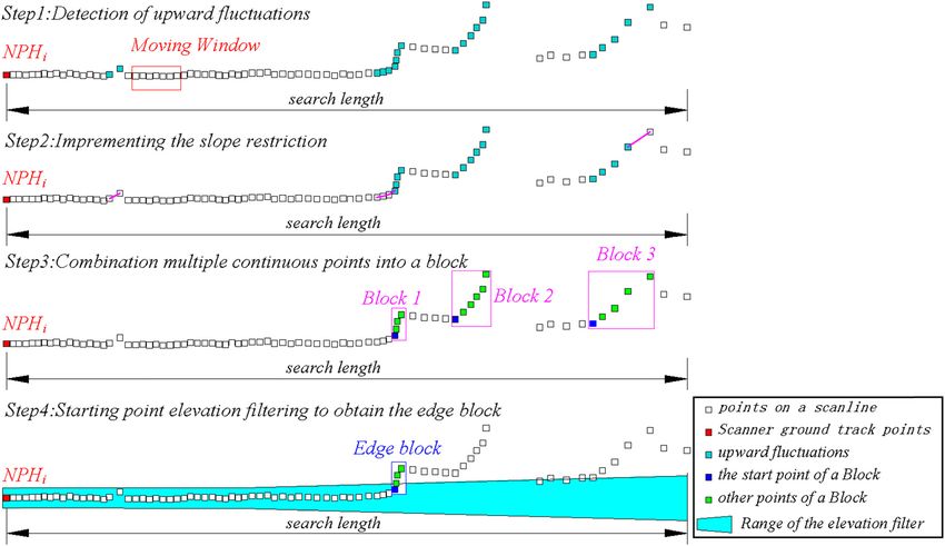
Extraction of road boundary from MLS data using laser scanner ground trajectory 699 Figure 11: Extracted edge blocks in Dataset 1. (a) Location of the starting point of the extracted edge blocks; (b) and (c) are enlarged maps of red and green boxes, respectively. noise [5,10,16,19], the proposed edge block detection constantly changes and tends to be gentle near the road method reduces noise as much as possible. In addition, surface. even if more than one boundary point corresponds to With slope restriction, a defined boundary point has NPHi, there is not much noise on the road surface. It is a slope greater than 30° to the next point. Alternatively, very likely that the first block extracted on each scan line poor data quality, affected by noise and wetness of the belongs to the road edge. Each edge block occupies a road surface, may be responsible. certain length, leaving multiple edge blocks on a scan There is a common phenomenon of missing point further apart than the hunting zone width used in the clouds, which is reflected in sudden changes in spacing edge tracking algorithm. As a result, there are only two between adjacent points in Figure 13(d). On the side view cases in boundary point tracking: there either is or is not shown in Figure 13(a), extracted boundary points are a point within the zone, which makes boundary tracking clustered together, whereas they are scattered in Figure efficient. Figure 13(b) and (d) shows the position of the 13(c). However, they remain the closest point to the starting point of the edge block. The extracted boundary boundary on this scanning line. points (red) accurately locate the road edge. The boundary Except for the minimal contact area between the points detected in Dataset 2 shown in Figure 13(d) are not lower part of a wheel and the road, the outline points as neat as those of the urban road in Figure 13(b). This of vehicles have abrupt changes in elevation and dis- may be because the gradient of S-shaped road curbstone tance. These changes are often geometrically backward, Figure 12: Extracted edge blocks in the winding road of Dataset 2. (a) Shows the location of the starting point of the extracted edge blocks; (b) and (c) are enlarged maps of green and red boxes, respectively.
700 Lichun Sui et al.
Figure 13: Location of extracted boundary points displayed on axonometric and side view. (a) Axonometric view in Dataset 1. (b) Side view in
Dataset 1. (c) Axonometric view in Dataset 2. (d) Side view in Dataset 2.
that is, the horizontal distance (d) from the scanner is Although travel direction (in Figure 14(e)) is not consis-
reduced, which is not in line with the law of the defined tent with the boundary, the spacing between the travel
characteristics of the boundary points. Only a very small direction and the boundary can be traced linearly. There
number of edge blocks at the lower part of wheels were is one boundary point omitted in T1 as it is beyond the
detected, and subsequently were ignored in boundary search length in both directions. Three points in T2
tracking process. Therefore, occlusions because of the exceed the hunting zone because of a sudden turn in
parking cars on the roadside cause little trouble to the the branch. This may also occur at the end of the arc
boundary points detection. green belt and road forks, but the number of such omitted
points is small. Ignoring the form of the boundary,
boundary points in the red circle in Figure 14(c) are
extracted; these are actually on the border rather than
3.4 Boundary tracking the curb. At Area 2, depicted in Figure 14(d), the boundary
is broken into very short, widely spaced parts. The quality
Table 2 lists the boundary points identified by the tracking of this point cloud acquisition is insufficient for boundary
algorithm. The completeness of the boundary tracking extraction. Moreover, long tracking length results in poor
step is above 99.2%. The continuous boundary on the reliability. However, this is a rare case. The disconnection
left side of the road in Dataset 1 was completely detected. overlap area has been searched twice from two directions
In addition, disconnected boundaries (the left side of to detect as lots of tracked points as possible, while con-
Dataset 2) and the branches (the right side of Datasets 1 trolling for the risk of omission and misjudgment.
and 2) result in the removal – during boundary tracking – In contrast, there is only a small amount of occlusion
of four, two, and two boundary points, respectively, as in Dataset 2. The vehicle trajectory is consistent with the
they do not conform to the main convergence direction of road boundary in most cases, which guarantees relia-
boundary points in the neighborhood. bility of the boundary tracking algorithm. Except for
The road boundary tracking results of Dataset 1 on loss of the track at the top of the greenbelt similar to T3
perspective are shown in Figure 14. In the figure, blue in Figure 15(d), ideal boundary tracking is achieved using
points denote NPH, and red points the starting point of spacing between the vehicle and the road edge as a
the edge blocks. Tracked points are also shown in green. model parameter. The tracking algorithm is not
Table 2: Tracing results of road boundary points
Experimental data Road boundary Number of road edge Identified boundary Missed boundary points in Detection rate (%)
blocks points tracking
Dataset 1 Left 832 832 0 100
Right 529 525 4 99.2
Dataset 2 Left 804 802 2 99.7
Right 620 618 2 99.6Extraction of road boundary from MLS data using laser scanner ground trajectory 701
Figure 14: Results of boundary tracking in Dataset 1. (a) Candidate boundary points and (b) boundary points recognized after tracking. (c),
(d), and (e) are enlargement maps of Area 1, Area 2, and Area 3, respectively.
dependent on the line shape of the road. To further verify points. Both sides of the bend show great extraction. At
the universality of the algorithm, a T-junction was selected the intersection of the road, where road boundaries are
for experiments. The results are shown in Figure 16. not continuous, the proposed method is more efficient
Travel speed varies greatly when turning, resulting in and convenient than fitting road boundaries based on
different NPH spacing. However, the estimated scanner multiple models.
ground trajectory (blue points) in Figure 16 is still smooth, With short occlusion length, the correctness and
illustrating the universal reliability of the presented integrity of boundary point extraction are guaranteed
method for estimating scanner trajectory. The boundary by the proximity and collinearity of boundary points
points of the main road continue to track along the ori- on a pseudo-mileage spacing map. Rather than directly
ginal direction (red points in the upper part of Figure establishing a tracking model for boundary lines that
16(b)) when the vehicle turns to the branch. Boundary may require many different models to fit different seg-
points on the lateral bend at the turning are quickly ments [21,41], the presented method uses simple linear
tracked because of aggregation of candidate boundary models to track spacing between the road boundary and
Figure 15: Results of boundary tracking in Dataset 2. (a) Candidate edge points and (b) boundary points recognized after tracking; (c) and (d)
are further enlargement maps of Area 4 and Area 5, respectively.702 Lichun Sui et al.
Figure 16: Extraction of boundary points at a T-junction. (a) The inner bend and (b) the outer bend.
the vehicle. The proposed algorithm does not require the lateral branch boundaries with a small number of edge
road boundary to be strictly parallel to the direction of points. In future research, we will focus on improving.
travel of the vehicle, nor is it related to the line shape of
the road boundary. Another advantage is the speed of the Acknowledgments: Thanks are due to Chuanshuai Zhang
algorithm. The execution time is extremely short as it uses for his data collection and technological help, and to Jun
the original recording order. Comparatively speaking, cal- Wang for assistance with the experiments.
culation of the scanner’s ground trajectory takes longer
than that of searching the road edge blocks and tracking Funding information: This study was supported by the
the boundary points, as they only operate in scan lines National Natural Science Foundation of China, Grant
located on PG. If vehicle trajectory data are available, the Nos. 41890854; 41372330; 41671436; Natural Science Basic
extraction process can be completed in real time. Research Plan in the Shaanxi Province of China, Grant No.
2021JQ-819.
Author contributions: L. C. S. and M. Q. Z. conceptualized
4 Conclusion the model. J. F. Z. and M. Q. Z. deduced the method and
designed the experiment. J. F. Z. and X. W. developed the
This study estimated a scanner’s ground track based model code. M. Q. Z. and J. M. K. performed the data
on the spatial distribution of point clouds. With the collation and accuracy verification. L. C. S. and J. F. Z.
estimated track point and multiple constraints of neigh- prepared the manuscript with contributions from all co-
borhood elevation difference, slope, and continuity of authors.
fluctuation points, accurate edge blocks with strong resis-
tance to noise are defined. Spacing between edge blocks Conflict of interest: Authors state no conflict of interest.
and the scanner track is transformed into a pseudo-
mileage spacing map. As the spacing varies little over a
short distance, the edge is easy to detect and track using a
simple linear model. Experiments on noisy data accu- References
rately extracted the location of edge blocks separated
far from one another on a scan line, which guarantees [1] Yang B, Wei Z, Li Q, Li J. Automated extraction of street-scene
the reliability of this linear tracking model and improves objects from mobile lidar point clouds. Int J Remote Sens.
tracking speed. Our results suggest that the proposed 2012;33(18):5839–61.
method is not dependent on whether the road boundary [2] Miyazaki R, Yamamoto M, Hanamoto E, Izumi H, Harada K.
is parallel to the direction of traveling path of the vehicle, A line-based approach for precise extraction of road and curb
region from mobile mapping data. ISPRS Ann Photogram
nor the line type of the road boundary. Road edge points
Remote Sens Spat Inf Sci. 2014;II(5):243–50.
can be extracted quickly, effectively, and accurately as [3] Wu B, Yu B, Huang C, Wu Q, Wu J. Automated extraction of
long as normal data acquisition quality can be guaran- ground surface along urban roads from mobile laser scanning
teed. However, the tracking model may fail to recognize point clouds. Remote Sens Lett. 2016;7(2):170–9.Extraction of road boundary from MLS data using laser scanner ground trajectory 703
[4] Yang B, Dong Z, Liu Y, Liang F, Wang Y. Computing multiple [21] Sun P, Zhao X, Xu Z, Wang R, Min H. A 3D LiDAR data-based
aggregation levels and contextual features for road facilities dedicated road boundary detection algorithm for autonomous
recognition using mobile laser scanning data. ISPRS J vehicles. IEEE Access. 2019;7:29623–38.
Photogram Remote Sens. 2017;126:180–94. [22] Boyko A, Funkhouser T. Extracting roads from dense point
[5] Xu S, Wang R, Zheng H. Road curb extraction from mobile clouds in large scale urban environment. ISPRS J Photogram
LiDAR point clouds. IEEE Trans Geosci Remote Sens. Remote Sens. 2011;66(6):S2–12.
2017;55(2):996–1009. [23] Guan H, Li J, Yu Y, Ji Z, Wang C. Using mobile LiDAR data for
[6] Kumar P, Mcelhinney CP, Lewis P, Mccarthy T. An automated rapidly updating road markings. IEEE Trans Intell Transp Syst.
algorithm for extracting road edges from terrestrial mobile 2015;16(5):2457–66.
LiDAR data. ISPRS J Photogram Remote Sens. [24] Zhang Y, Wang J, Wang X, Li C, Wang L. 3D LIDAR-based
2013;85(11):44–55. intersection recognition and road boundary detection method
[7] Ibrahim S, Lichti D. Curb-based street floor extraction from for unmanned ground vehicle. 2015 IEEE 18th International
mobile terrestrial lidar point cloud. ISPRS – Int Arch Conference on Intelligent Transportation Systems,
Photogram Remote Sens Spat Inf Sci. 2012;39:193–8. September 15–18, 2015. Gran Canaria, Spain: IEEE; 2015.
[8] Zai D, Li J, Guo Y, Cheng M, Lin Y, Luo H, et al. 3-D road p. 499–504.
boundary extraction from mobile laser scanning data via [25] Yu Y, Li J, Guan H, Jia F, Wang C. Learning hierarchical features
supervoxels and graph cuts. IEEE Trans Intell Transp Syst. for automated extraction of road markings from 3-D Mobile
2018;19(3):802–13. LiDAR point clouds. IEEE J Sel Top Appl Earth Observ Remote
[9] Guo J, Tsai M-J, Han J-Y. Automatic reconstruction of road Sens. 2015;8(2):709–26.
surface features by using terrestrial mobile lidar. Autom [26] Xia S, Chen D, Wang R. A breakline-preserving ground inter-
Constr. 2015;58:165–75. polation method for MLS data. Remote Sens Lett.
[10] Zhang W, editor. LIDAR-based road and road-edge detection. 2019;10(12):1201–10.
2010 IEEE Intelligent Vehicles Symposium, June 21–24, 2010. [27] Lin Y, Wang C, Zhai D, Li W, Li J. Toward better boundary pre-
La Jolla, CA, USA: IEEE; 2010. p. 845–8. served supervoxel segmentation for 3D point clouds. ISPRS
[11] Hervieu A, Soheilian B, editors. Road side detection and J Photogram Remote Sens. 2018;143(Sep):39–47.
reconstruction using LIDAR sensor. 2013 IEEE Intelligent [28] Sha Z, Chen Y, Li W, Wang C, Nurunnabi A, Li J. A boundary-
Vehicles Symposium (IV), June 23–26, 2013. Gold Coast, enhanced supervoxel method for extraction of road edges in
Australia: IEEE; 2013. p. 1247–52. MLS point clouds. ISPRS – Int Arch Photogram Remote Sens
[12] Sherif Ibrahim DL. Curb-based street floor extraction from Spat Inf Sci. 2020;XLIII(B1-2020):65–71.
mobile terrestrial lidar point cloud. International Archives of [29] Xu Y, Ye Z, Yao W, Huang R, Stilla U. Classification of LiDAR
the Photogrammetry, Remote Sensing and Spatial Information point clouds using supervoxel-based detrended feature and
Sciences, Volume XXXIX-B5, 2012, XXII ISPRS Congress, perception-weighted graphical model. IEEE J Sel Top Appl
25 August–01 September 2012, Melbourne, Australia; 2012. Earth Observ Remote Sens. 2019;13:72–88.
p. 193–8 [30] Ibrahim S, Lichti D. Curb-based street floor extraction from
[13] Yadav M, Singh AK, Lohani B. Extraction of road surface from mobile terrestrial lidar point cloud. Int Arch Photogram Remote
mobile LiDAR data of complex road environment. Int J Remote Sens Spat Inf Sci. 2012;XXXIX(B5):193–8.
Sens. 2017;38(16):4655–82. [31] Han J, Kim D, Lee M, Sunwoo M. Enhanced road boundary and
[14] El-Halawany SI, Lichti DD. Detecting road poles from mobile obstacle detection using a downward-looking LIDAR sensor.
terrestrial laser scanning data. GISci Remote Sens. IEEE Trans Vehicular Technol. 2012;61(3):971–85.
2013;50(6):704–22. [32] Yang M, Wan Y, Liu X, Xu J, Wei Z, Chen M, et al. Laser data
[15] Yang B, Fang L, Li J. Semi-automated extraction and delinea- based automatic recognition and maintenance of road
tion of 3D roads of street scene from mobile laser scanning markings from MLS system. Opt Laser Technol.
point clouds. ISPRS J Photogram Remote Sens. 2018;107:192–203.
2013;79:80–93. [33] Antonio Martín-Jiménez J, Zazo S, Arranz Justel JJ, Rodríguez-
[16] Liu Z, Wang J, Liu D. A new curb detection method for Gonzálvez P, González-Aguilera D. Road safety evaluation
unmanned ground vehicles using 2D sequential laser data. through automatic extraction of road horizontal alignments
Sens (Basel). 2013;13(1):1102–20. from mobile LiDAR System and inductive reasoning based on a
[17] Jung J, Che E, Olsen MJ, Parrish C. Efficient and robust lane decision tree. ISPRS J Photogram Remote Sens.
marking extraction from mobile lidar point clouds. ISPRS J 2018;146:334–46.
Photogram Remote Sens. 2019;147:1–18. [34] Yalcin O, Sayar A, Arar OF, Akpinar S, Kosunalp S. Approaches
[18] Rodríguez Cuenca B, García Cortés S, Ordóñez, Galán C, of road boundary and obstacle detection using LIDAR. IFAC
Alonso MC. An approach to detect and delineate street curbs Proc Volumes. 2013;46(25):211–5.
from MLS 3D point cloud data. Autom Constr. 2015;51:103–12. [35] Wang H, Cai Z, Luo H, Cheng W, Li J, editors. Automatic road
[19] Serna A, Marcotegui B. Urban accessibility diagnosis from extraction from mobile laser scanning data. International
mobile laser scanning data. ISPRS J Photogram Remote Sens. Conference on Computer Vision in Remote Sensing,
2013;84:23–32. December 16–18, 2012. Xiamen, China: IEEE; 2013.
[20] Wijesoma WS, Kodagoda K, Balasuriya AP, editors. Road- p. 136–9.
boundary detection and tracking using ladar sensing. IEEE [36] Anttoni J, Juha H, Hannu H, Sensors KAJ. Retrieval algorithms
Transactions on Robotics and Automation. Lausanne, for road surface modelling using laser-based mobile mapping.
Switzerland: IEEE; 2004;20(3). p. 456–4. Sens (Basel). 2008;8(9):5238–49.704 Lichun Sui et al.
[37] Wang H, Luo H, Wen C, Cheng J, Li P, Chen Y, et al. Road [40] Goulette F, Nashashibi F, Abuhadrous I, Ammoun S,
boundaries detection based on local normal saliency from Laurgeau C. An integrated on-board laser range sensing
mobile laser scanning data. IEEE Geosci Remote Sens Lett. system for on-the-way city and road modelling. In Proceedings
2015;12(10):2085–9. of the ISPRS Commission I Symposium “From Sensors to
[38] Zhang Y, Wang J, Wang X, Dolan JM. Road-segmentation-based Imagery”, Paris, France; July 2006.
curb detection method for self-driving via a 3D-LiDAR sensor. [41] Wang X, Cai Y, Shi T, editors. Road edge detection based on
IEEE Trans Intell Transport Syst. 2018;19(12):3981–91. improved RANSAC and 2D LIDAR Data. 2015 International
[39] Guan H, Li J, Yu Y, Wang C, Chapman M, Yang B. Using mobile Conference on Control, Automation and Information Sciences
laser scanning data for automated extraction of road mark- (ICCAIS), October 29–31, 2015. Changshu, China: IEEE.
ings. ISPRS J Photogram Remote Sens. 2014;87:93–107. p. 191–6.You can also read


