GENERATING ARTIFICIAL NEAR INFRARED SPECTRAL BAND FROM RGB IMAGE USING CONDITIONAL GENERATIVE ADVERSARIAL NETWORK - DLR
←
→
Page content transcription
If your browser does not render page correctly, please read the page content below
ISPRS Annals of the Photogrammetry, Remote Sensing and Spatial Information Sciences, Volume V-3-2020, 2020
                                             XXIV ISPRS Congress (2020 edition)

 GENERATING ARTIFICIAL NEAR INFRARED SPECTRAL BAND FROM RGB IMAGE
       USING CONDITIONAL GENERATIVE ADVERSARIAL NETWORK

                                             Xiangtian Yuan1 ∗, Jiaojiao Tian1 , Peter Reinartz1
                      1
                          Remote Sensing Technology Institute (IMF), German Aerospace Center (DLR), Germany -
                                          (Xiangtian.yuan, Jiaojiao.tian, Peter.reinartz)@dlr.de

KEY WORDS: Near-infrared, RGB, Gerative adversarial networks, Robust loss function, Conditional GAN

ABSTRACT:

Near infrared bands (NIR) provide rich information for many remote sensing applications. In addition to deriving useful indices to
delineate water and vegetation, near infrared channels could also be used to facilitate image pre-processing. However, synthesizing
bands from RGB spectrum is not an easy task. The inter-correlations between bands are not clearly identified in physical models.
Generative adversarial networks (GAN) have been used in many tasks such as generating photorealistic images, monocular depth
estimation and Digital Surface Model (DSM) refinement etc. Conditional GAN is different in that it observes some data as a
condition. In this paper, we explore a cGAN network structure to generate a NIR spectral band that is conditioned on the input
RGB image. We test different discriminators and loss functions, and evaluate results using various metrics. The best simulated NIR
channel has a mean absolute error of around 5 percent in Sentinel-2 dataset. In addition, the simulated NIR image can correctly
distinguish between various classes of landcover.

                      1. INTRODUCTION                                   spectral nonlinear mapping, and a spatial sub network, which
                                                                        models the spatial correlation. Then hyperspectral bands are
In remote sensing, near-infrared bands (NIR) have been playing          generated by minimizing a mean squared error between gener-
important roles in many aspects. They exhibit additional po-            ated bands and real bands.
tential for representing ground objects in comparison to RGB
bands, especially in representing vegetations. For example, in-         In recent years, generative adversarial networks (GANs) have
dices involving NIR have been developed and used for tasks              been extensively used in remote sensing community to tackle
such as landcover classification. These indices includes Nor-           various tasks. For example, GAN and its variants are capable
malized Vegetation Index (NDVI) and Normalized water index              or refining Digital Surface Models (DSMs) derived from stereo
(NDWI), which have been proven to be effective in highlighting          matching (Bittner et al., 2019). In addition, GANs are applied
vegetation and open water feature in remote sensing imagery             in hyperspectral image classification (Zhan et al., 2017), PAN-
(McFeeters, 1996). In addition to identifying vegetation and            sharpening (Liu et al., 2018) and super resolution (Ledig et al.,
water, NIR band is also capable of discerning materials such as         2017) tasks.
plastic, minerals, sea foams, trace gases, and the health prob-
lems of trees. In data-hungry machine learning or deep learn-           Due to the versatility of GANs, we want to test if GANs are
ing methods for landcover classification, these characteristics         capable of generating realistic NIR band reflectance. The gen-
enable NIR bands to be used to improve coarse ground truth,             erated NIR bands should keep the original image textures, as
and correct wrong labels with their capability of distinguish-          well as the physical radiometric properties. To this purpose,
ing between classes with subtle difference in spectral signature.       GAN in conditional setting is more suitable, meaning that the
Moreover, NIR-derived indices have also been used in some               generated NIR bands will be conditioned on the visible spec-
tasks such as atmospheric correction (Kaufman, Sendra, 1988).           tra (red, green and blue). This conditional setting ensures that
                                                                        the generated NIR bands are not only realistic, but also close
But NIR bands are not always available in every sensor. Some            to RGB input in terms of information content. To this end, ad-
low cost satellite might not be equipped with sensor capable of         ditional loss functions such as L1 or L2 are added to the GAN
capturing NIR bands. Some airborne systems also only consist            loss to ensure that the output is close to the ground truth (Isola
of cameras capturing RGB bands. Moreover, sometimes when                et al., 2017). However, such losses are susceptible to outliers.
doing landcover change detection, data from old sensors might           Some robust loss functions are able to handle outliers by put-
not provide NIR bands as the newer ones, thus hindering the ac-         ting less sensitivity to large error. A single robust loss function
curacy of change detection. Therefore, synthesizing NIR bands           proposed by (Barron, 2019) encompasses several common ro-
from RGB is of practical values.                                        bust loss functions. This robust loss function is controlled by a
                                                                        single continuous-valued parameter that can also be optimized
The generation of NIR band from RGB can be regarded as a                when training neural networks.
nonlinear mapping from RGB to NIR. Neural networks have
been proven to be effective in nonlinear mapping. For example,          In this work, we will present a method to generate NIR band
one paper (Fu et al., 2018) proposed a network structure for            from RGB bands, which applies a robust loss function in condi-
hyperspectral image reconstruction from RGB bands. The net-             tional GAN setting. We tested the method on Sentinel-2 Data-
work consists of a spectral sub network, which performs the             set and analysed the applicability of the proposed method. The
                                                                        contribution of our work is twofold: we tested a conditional
  ∗ Corresponding   author                                              GAN for task that not only requires perceptive realness but also

         This contribution has been peer-reviewed. The double-blind peer-review was conducted on the basis of the full paper.
                     https://doi.org/10.5194/isprs-annals-V-3-2020-279-2020 | © Authors 2020. CC BY 4.0 License.                       279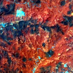
ISPRS Annals of the Photogrammetry, Remote Sensing and Spatial Information Sciences, Volume V-3-2020, 2020
                                             XXIV ISPRS Congress (2020 edition)

NIR band with meaningful radiometric properties; we also ad-          2017). It classifies whether a N × N patch in the input im-
opted a robust loss function that contributes to better learning      age is real or fake, and average all the patches in the image.
in the generative model.                                              The discriminator is made of several blocks consisting of 2D
                                                                      convolution, batch normalization and leaky ReLU layers. The
The paper is structured as follows. In chapter two we describe        stride of all convolutions are 2 except for the last and second
in detail the concepts and methodology involved; in chapter           last convolutions. The size of receptive field of previous block
three, dataset and experiment settings are detailed. Results are      is calculated as:
analysed in chapter four, followed by conclusions in chapter
five.                                                                            (outputsize − 1) × stride + kernelsize               (1)

                                                                      It should be noted that the patch size of the patch discriminator
                    2. METHODOLOGY
                                                                      is defined as the size of receptive field in input that corresponds
                                                                      to one output pixel. Therefore, the deeper the discriminator,
GANs are built on game theory (Goodfellow et al., 2014) and
                                                                      the larger the patch size. The detail of a 3-layer (excluding the
have been used in multitudes of tasks in computer vision. In
                                                                      last two layers) PatchGAN discriminator is shown in Figure 1.
remote sensing, GANs have been proven to be effective in many
                                                                      Ignoring padding, the patch size is 70 × 70 for such 3-layer
applications and have achieved good results. The characteristics
                                                                      patch discriminator. It could be understood as a form of texture
of cGAN will be briefly described in this chapter.
                                                                      loss (Isola et al., 2017).
2.1   Conditional GAN
                                                                      Another option is a pixel level discriminator, which only clas-
                                                                      sifies real or fake on pixel level. Different from PatchGAN, the
GAN comprises generator and discriminator. The generator
                                                                      kernel size and stride equal to 1. Therefore, the feature map
tries to produce output while the discriminator tries to classify
                                                                      size remains unchanged across the network and no texture in-
if the output is fake or real (Goodfellow et al., 2014). The input
                                                                      formation is considered by discriminator. An illustration of the
of GAN is usually random noise vector, and the output is image
                                                                      pixel discriminator is shown in Figure 2.
that is similar to realistic images. Different from conventional
GANs, conditional GANs (Mirza, Osindero, 2014) observe in-
                                                                      Both discriminators’ last layer is a binary cross entropy layer
put data. In our case, the network should generate NIR band
                                                                      that classifies if the generated image is true or false. The result
while observing RGB bands. Then the discriminator tries to
                                                                      is averaged over the whole image.
distinguish between the real and the fake image from generator
until it can not distinguish anymore. In cGAN, the discrimin-
ator is also conditioned on the input RGB bands similar to the
generator. Therefore, NIR band corresponding to RGB bands
can be generated from the cGAN.

2.1.1 Generator Generating realistic NIR band from RGB
bands can be regarded as a mapping from input to output of the
same spatial resolution. As the input and output are representa-
tion of the same ground objects, they should match in structure,
                                                                         Figure 1. Illustration of PatchGAN Discriminator. The first
texture and have same semantics. A number of GAN generat-
                                                                       block has no batch normalization. The first three convolutions
ors adopt encoder-decoder structures that first reduce the spatial
                                                                           have a filter size of 4 × 4 and stride of 2. The last two
resolution of input and gradually recover it. This structure loses
                                                                      convolution layers has stride of 1, therefore retaining the spatial
the low level information from previous stages, resulting in lack
of details. Therefore, encoder-decoder network with skip con-           resolution. The output is passed on to a binary cross entropy
nection is more suitable for this task. This structure is capable             function. The output is a score for whole image.
of retaining information from different stages in the network,
which is popularly known as U-Net structure (Ronneberger et
al., 2015). This generator is adopted in image-to-image trans-
lation model Pix2pix (Isola et al., 2017). The U-net in our ex-
periment consists of 8 blocks in both encoder and decoder. In
encoder each block encompasses convolution, batch normaliz-
ation and LeakyReLU of slope 0.2. In decoder each block com-
prises transposed convolution, batch normalization and ReLU
layers. The convolution has a filter size of 4 and stride of 2 in
both encoder and decoder. In some conditional GANs, Gaus-              Figure 2. Illustration of Pixel Discriminator. The convolution
sian noise z is provided to generator as input to avoid determ-       filters have a size of 1 × 1 and stride of 1. The classification of
inistic results matching delta function (Isola et al., 2017). Dif-       real and fake is only on pixel level, without any contextual
ferent from this approach, Pix2pix model employs drop out in             information. The result after binary cross entropy (BCE) is
generator during both training and testing phase. Although this                                    averaged.
approach results in reduced stochasticity, it is still suitable for
our task as our task does not need much randomness as other           2.2   Loss Function Formulation
computer vision tasks such as image translation.
                                                                      2.2.1 GAN Loss In GANs, random noise z conforming to
2.1.2 Discriminator As for discriminator, various options             certain probability distribution is mapped to the desired output
are available depending on the task. One choice is the Markovian      y by generator G. Conditional GAN, on the other hand, learns a
discriminator, which is also termed as PatchGAN (Isola et al.,        mapping not solely from random noise z , but from both random

         This contribution has been peer-reviewed. The double-blind peer-review was conducted on the basis of the full paper.
                     https://doi.org/10.5194/isprs-annals-V-3-2020-279-2020 | © Authors 2020. CC BY 4.0 License.                      280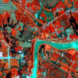
ISPRS Annals of the Photogrammetry, Remote Sensing and Spatial Information Sciences, Volume V-3-2020, 2020
XXIV ISPRS Congress (2020 edition)
noise z and input image x. G : {x, z} → y . Discriminator D is The logarithmic of the partition function can be approxim-
trained adversarially against generator G to distinguish between ated using the cubic Hermit spline. The negative log likelihood
real image and generated image. The objective function of con- of the distribution can avoid skewing towards ignoring outlier
ditional GAN can be expressed as: by forcing extra penalty for small errors. The details can be
found in paper (Barron, 2019). Therefore, the final objective
LcGAN (G, D) = Ex,y [LogD(x, y)] for cGAN with robust loss function can be expressed as:
(2)
+ Ex,z [log(1 − D(G(x, z)))]
arg min max = LcGAN (G, D) + λLRobust (G) (9)
G D
The loss of the unconditional GAN can be written as:
LGAN (G, D) = Ey [LogD(y)]
(3) 3. EXPERIMENT
+ Ez [log(1 − D(G(z)))]
We use the multispectral images from SEN12MS dataset based
on Sentinel-1 and Sentinel-2 dataset (Schmitt et al., 2019). The
2.2.2 Traditional Loss It has been found beneficial to com- Sentinel-2 data from SEN12MS is level 1-C Top of Atmosphere
bine GAN loss with traditional loss functions such as L1 or reflectance (TOA) product. The images have in total 13 band
L2 (Isola et al., 2017). In our task, the generated NIR band with spatial resolution from 10m to 60 m. In our experiment,
should not only be distinguishable from the real NIR band, but we selected the red (R), green (G), blue (B) and near-infrared
also has to be close to the real NIR band numerically. There- (NIR) bands with 10 m resolution. The dataset encompasses
fore, traditional loss is helpful in enforcing results to be close areas including desert, field, forests, urban areas, water bodies
to ground truth. Compared with L2, L1 loss encourages less etc. Example images are shown in Figure.4. The images in
blurring (Isola et al., 2017). L1 loss is calculated as: SEN12MS are distributed across the world as can be seen from
Figure.3. It shows that the data are distributed globally, with
LL1 (G) = Ex,y,z [ z − G(x, z) ] (4)
1 varying latitudes and climate conditions. The landcover type
also varies drastically in different locations. The dataset is cat-
The final loss can be expressed as:
egorised by seasons. In this paper, we used data acquired in
summer for training and testing to avoid problems incurred by
arg min max = LcGAN (G, D) + λLL1 (G) (5)
G D properties of multi-seasonal dataset. Details of band informa-
tion can be seen in Table.1.
2.2.3 Robust Loss L1 and L2 losses suffer from the prob-
lem of outliers, meaning that outlier contributes equally to loss
as inlier. The ability to handle outliers is termed robustness in
machine learning. Robustness is a crucial property that is de-
sired in machine learning models. There are several robust loss
functions that have reduced sensitivity to large errors, such as
Cauchy/Lorentzian (Black, Anandan, 1996), Geman-McClure
(Geman, McClure, 1985), Welsch (Dennis Jr, Welsch, 1978),
Charbonnier (Charbonnier et al., 1994) and generalized Char-
bonnier (Sun et al., 2010). These loss functions have saturating
or even reduced gradient when the loss is large. A robust loss
function proposed by (Barron, 2019) is the superset of many
common robust loss functions mentioned above. It is able to
adjust its robustness as a continuous parameter during training. Figure 3. Visualization of locations of images in the experiment.
The loss function is defined as: Blue dots denote the location of clusters of smaller images.
!α/2
|α − 2| (x/c) 2 Wavelength(nm) Bandwidth Resolution
f (x, α, c) = +1 − 1 (6) Bands
α |α − 2| S2A S2B (nm) (m)
Red 664.6 664.9 31 10
Green 559.8 559.0 36 10
It is a generalisation of many losses. In Equation 6, α controls
the robustness of the loss; c > 0 is the scale parameter that Blue 492.4 492.1 66 10
controls the size of quadratic bowl nean x = 0. A general NIR 832.8 832.9 106 10
probability distribution can be constructed from the robust loss,
so that the log-likelihood of the probability density is a shifted Table 1. Data Description from (European Space Agency, 2015).
version of the robust loss function. The distribution is defined S2A and S2B are the two satellites respectively. Wavelength is
as: the central wavelength
1
p(x|µ, α, c) = exp(−f (x − µ, α, c)) (7)
cZ(α) 3.1 Data Pre-processing
We randomly selected 30000 images from the summer scenes
In this equation, Z(α) is a partition function: for training and 300 images for testing. In Sentinel-2 Level-1C
data, the digital number (DN) is TOA reflectance multiplied by
Z ∞
10000. We therefore converted the DN to physically meaning-
Z(α) = exp(−f (x, α, 1)) (8) ful reflectance and zero-centered the pixel value for training. In
−∞
This contribution has been peer-reviewed. The double-blind peer-review was conducted on the basis of the full paper.
https://doi.org/10.5194/isprs-annals-V-3-2020-279-2020 | © Authors 2020. CC BY 4.0 License. 281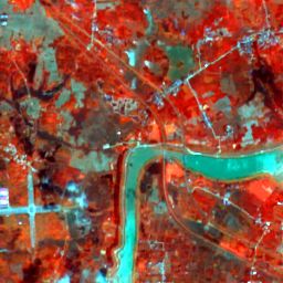
ISPRS Annals of the Photogrammetry, Remote Sensing and Spatial Information Sciences, Volume V-3-2020, 2020
XXIV ISPRS Congress (2020 edition)
SSIM (x, y) = [l(x, y)]α · [c(x, y)]β · [s(x, y)]γ (12)
In the above SSIM definition, α, β, γ are parameters that define
the relative importance of the three components. The mean in-
tensities are µx and µy , standard deviations are σx and σy , C1
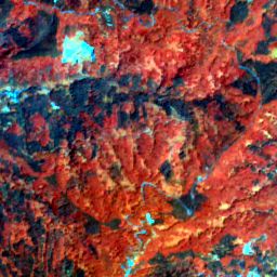
(a) Image with (b) Image with (c) Image with (d) Image with
mostly high mostly low mostly barren around half
and C2 are constants that are used to avoid zero denominator
vegetation vegetation and landscape water and half instability, and are related to dynamic range of pixel values.
urban area high vegetation Mean intensity and standard deviation are weighted by a Gaus-
sian weighting function of σ = 1.5. If we set α, β and γ all
Figure 4. Example images from different regions with various equal to 1, the equation becomes:
landcover types. As can be seen from images, landcover is very
distinct from region to region.
(2µx µy + C1 )(2σxy + C2 )
generative models, data pre-processing is very crucial for learn- SSIM (x, y) = (13)
ing, and we find this pre-processing strategy effective. (µ2x + µ2y + C1 )(σx2 + σy2 + C2 )
3.2 Training Settings
In addition to approximating the reflectance values, we expect
We test cGAN networks with pixel discriminator and patch dis- the near-infrared channel to correctly reflect the characteristic
criminator. We also test a U-net generator without cGAN set- of various landcover types. Specifically, the generated NDVI
ting in order to verify if the cGAN objective facilitates better should also have low value at water bodies and high values
learning. Among these models, we compare traditional L1 loss at vegetation areas. We implement a simple classification rule
and robust loss in the final objective. The experiment is per- which performs quantization on the NDVI and derives four classes
formed based on Pytorch framework. We used Adam optimizer that can be roughly summarized as water, baren, low veget-
(Kingma, Ba, 2014) and learning rate of 0.0002. The parameter ation, high vegetation. The classe definition is illustrated in
of the robust loss function is optimized together with network Equation.14. It should be noted that the classification is an over
parameters. Batch size is set to 16. The input patch size is generalization for all the landcover types in the dataset. But
256 × 256 without any cropping or rotation. The parameter as we only want to test if fake NIR is capable of separating
weights are initialized by uniform distribution between 0 to 1. classes with distinctive spectral characteristics, the classifica-
The λ is set to 100 for the cGAN because the L1 loss is signi- tion scheme is still meaningful used in our evaluation.
ficantly smaller than cGAN loss. We train the network for 200
epoch. In training process, dropout is employed in generator to P ixel = W ater, if :
serve as random noise. −1
ISPRS Annals of the Photogrammetry, Remote Sensing and Spatial Information Sciences, Volume V-3-2020, 2020
                                             XXIV ISPRS Congress (2020 edition)

the highest mIoU scores for NDVI classification. The cGAN-            However, the best results still show some degree of information
PixelD model also acquires the lowest MAE and MAPE for                loss compared with the original NIR band. Specifically, the
both NDWI and NDVI. As for loss function, robust loss shows           generated images are relatively blurry in edges compared with
improvement over L1 loss function in every model variation.           the original NIR band. The reduced texture is possibly caused
On the other side, cGAN-PatchD with L1 loss function results          by the convolution operation and down sampling.
the worst performance in all the evaluation. In this model vari-
ation, robust loss has demonstrated the biggest improvement
over L1 loss.
                                                                                           5. CONCLUSION

         Network        Loss    MAE      MAPE SSIM                    NIR band is important in remote sensing applications as it provides
                                (×10−3 ) (%)                          additional information about landcover types. They have also
                                                                      shown significance in many interdisciplinary researches. How-
                   L1             10.70      5.54   93.08
           U-Net                                                      ever, not every equipment is capable of capturing NIR bands, or
                  Robust          10.60      5.46   93.13             sometimes NIR bands are missing in time series dataset. Gen-
                   L1             19.95     14.33   79.89             erating NIR band from RGB bands has very important practical
      cGAN-PatchD
                  Robust          10.85      5.19   92.28             uses. Generative adversarial models have been proven to have
                   L1              9.99      4.82   93.43             good performance in many generative tasks. They have been
      cGAN-PixelD                                                     transferred to many applications in remote sensing field such as
                  Robust           9.67      4.73   93.63
                                                                      DSM refinement and monocular depth estimation. In this pa-
                                                                      per, we have shown that cGAN is a viable method to be used in
  Table 2. The result comparison of different methods. MAE,           NIR band generation from RGB bands. The quality of the gen-
    MAPE and SSIM of generated NIR band is calculated.                erated NIR band is numerically good, with around 5 percent
                                                                      of mean absolute percentage error. In addition, it can in gen-
        Network        Loss    MAE      MAE      mIoU                 eral reflect accurate land cover class information through vari-
                               (×10−3 ) (×10−3 ) (%)                  ous NIR-based indices. However, the model still suffers from
                                                                      some texture loss that could potentially harm the usability of
                               NDWI     NDVI                          generated data. In the future, we will try to design a better gen-
                  L1             21.85      20.76    95.39            erator structure that can retain more texture information, and a
          U-net                                                       stronger discriminator that can distinguish between more subtle
                 Robust          21.79      20.70    95.34
                                                                      differences. In addition, imagery from different seasons will
                  L1             55.56      58.81    87.43            later be tested in following research to verify if the method is
     cGAN-PatchD
                 Robust          21.80      20.11    95.41            applicable when atmospheric property is distinct. Training and
                  L1             21.97      18.85    95.68            testing on multi-sensor dataset will also be experimented.
     cGAN-PixelD
                 Robust          18.90      17.61    95.79
                                                                                       ACKNOWLEDGEMENTS
 Table 3. The MAE results for NDWI and NDVI respectively,
and the mIoU based on NDVI classification. The mIoU score is          We would like to thank the authors of cited papers for interest-
              the average among all four classes.                     ing ideas and methodology. We are also grateful to researchers
                                                                      for generously disclosing the code that makes research more
In Figure. 5, 6 and 7 we present some example results from            efficient.
various models. We find that the lowest MAE is always achieved
in noisy images due to the relative low absolute reflectance val-
ues. These NIR bands have even discrete values. Therefore we                                 REFERENCES
exclude noisy images in visualization. We select some random
images to show the performance in different landcover types,          Barron, J. T., 2019. A general and adaptive robust loss function.
including water, forest, mountain, field and urban areas. We          Proceedings of the IEEE Conference on Computer Vision and
present the result in false color for better visualization. NDVI      Pattern Recognition, 4331–4339.
indices are shown in jet color map for visual comparison. We
plot the histograms of fake and real NIR bands to compare the         Bittner, K., Körner, M., Fraundorfer, F., Reinartz, P., 2019.
probability distributions. The blue one denotes the original NIR      Multi-Task cGAN for Simultaneous Spaceborne DSM Refine-
while orange one is that of fake NIR band. Except for some            ment and Roof-Type Classification. Remote Sensing, 11(11),
noisy images, almost all the fake NIR images demonstrate high         1262.
level of realness compared with the real ones. The cGAN-
                                                                      Black, M. J., Anandan, P., 1996. The robust estimation of mul-
PixelD model acquired best results in all evaluation metrics.
                                                                      tiple motions: Parametric and piecewise-smooth flow fields.
As can be seen in figure.5e and figure.5j, the histograms of the
                                                                      Computer vision and image understanding, 63(1), 75–104.
generated NIR bands in general match reasonably well with the
histograms of the real NIR bands. Patch discriminator cGAN            Charbonnier, P., Blanc-Feraud, L., Aubert, G., Barlaud,
model, on the other hand, shows decreased performance. It is          M., 1994. Two deterministic half-quadratic regularization al-
the only combination that has mIoU below 90 percent. As we            gorithms for computed imaging. Proceedings of 1st Interna-
can see in figure.6e and figure.6j, the distributions show big dif-   tional Conference on Image Processing, 2, IEEE, 168–172.
ferences and shifts from that of the real NIR bands. The NDVI
values also have large difference in some specific areas. The         Dennis Jr, J. E., Welsch, R. E., 1978. Techniques for non-
U-net model can also yield reasonable results without cGAN            linear least squares and robust regression. Communications in
objectives, but the result is not as good as cGAN-PixelD model.       Statistics-simulation and Computation, 7(4), 345–359.

         This contribution has been peer-reviewed. The double-blind peer-review was conducted on the basis of the full paper.
                     https://doi.org/10.5194/isprs-annals-V-3-2020-279-2020 | © Authors 2020. CC BY 4.0 License.                   283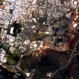
ISPRS Annals of the Photogrammetry, Remote Sensing and Spatial Information Sciences, Volume V-3-2020, 2020
XXIV ISPRS Congress (2020 edition)
(a) False color image (b) False color image (c) NDVI image from (d) NDVI image from (e) Histogram comparison
with real NIR band with fake NIR band real NIR band fake NIR band between real and fake NIR bands
(f) False color image (g) False color image (h) NDVI image from (i) NDVI image from (j) Histogram comparison
with real NIR band with fake NIR band real NIR band fake NIR band between real and fake NIR band
Figure 5. The results of U-net with l1 loss.
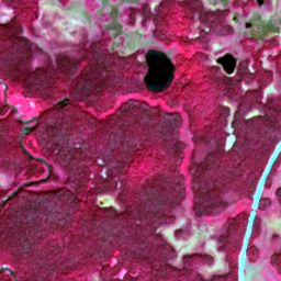
(a) False color image (b) False color image (c) NDVI image from (d) NDVI image from (e) Histogram comparison
with real NIR band with fake NIR band real NIR band fake NIR band between real and fake NIR bands
(f) False color image (g) False color image (h) NDVI image from (i) NDVI image from (j) Histogram comparison
with real NIR band with fake NIR band real NIR band fake NIR band between real and fake NIR band
Figure 6. The result of cGAN-PatchD with l1 loss.
(a) False color image (b) False color image (c) NDVI image from (d) NDVI image from (e) Histogram comparison
with real NIR band with fake NIR band real NIR band fake NIR band between real and fake NIR bands
(f) Real NIR band in (g) Fake NIR band in (h) NDVI image from (i) NDVI image from (j) Histogram comparison
false color false color real NIR band fake NIR band between real and fake NIR band
Figure 7. The result of cGAN-PixelD with robust loss.
This contribution has been peer-reviewed. The double-blind peer-review was conducted on the basis of the full paper.
https://doi.org/10.5194/isprs-annals-V-3-2020-279-2020 | © Authors 2020. CC BY 4.0 License. 284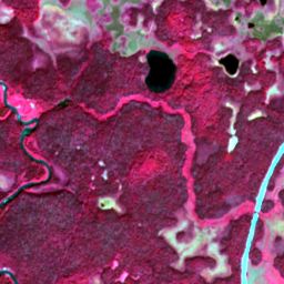
ISPRS Annals of the Photogrammetry, Remote Sensing and Spatial Information Sciences, Volume V-3-2020, 2020
                                             XXIV ISPRS Congress (2020 edition)

European Space Agency, 2015. SENTINEL-2 User Handbook.               Zhan, Y., Hu, D., Wang, Y., Yu, X., 2017. Semisupervised hy-
[Online]. Available from:    http://sentinel.esa.int/                perspectral image classification based on generative adversarial
documents/247904/685211/Sentinel-2_User_Handbook.                    networks. IEEE Geoscience and Remote Sensing Letters, 15(2),
[Accessed 15th Jan 2020].                                            212–216.

Fu, Y., Zhang, T., Zheng, Y., Zhang, D., Huang, H., 2018. Joint
camera spectral sensitivity selection and hyperspectral image
recovery. Proceedings of the European Conference on Com-
puter Vision (ECCV), 788–804.

Geman, S., McClure, D., 1985. Bayesian image analysis: An
application to single photon emission tomography. Amer. Stat-
ist. Assoc, 12–18.

Goodfellow, I., Pouget-Abadie, J., Mirza, M., Xu, B., Warde-
Farley, D., Ozair, S., Courville, A., Bengio, Y., 2014. Generat-
ive adversarial nets. Advances in neural information processing
systems, 2672–2680.

Isola, P., Zhu, J.-Y., Zhou, T., Efros, A. A., 2017. Image-to-
image translation with conditional adversarial networks. Pro-
ceedings of the IEEE conference on computer vision and pat-
tern recognition, 1125–1134.

Kaufman, Y. J., Sendra, C., 1988. Algorithm for automatic at-
mospheric corrections to visible and near-IR satellite imagery.
International Journal of Remote Sensing, 9(8), 1357–1381.

Kingma, D. P., Ba, J., 2014. Adam: A method for stochastic
optimization. arXiv preprint arXiv:1412.6980.

Ledig, C., Theis, L., Huszár, F., Caballero, J., Cunningham,
A., Acosta, A., Aitken, A., Tejani, A., Totz, J., Wang, Z. et al.,
2017. Photo-realistic single image super-resolution using a gen-
erative adversarial network. Proceedings of the IEEE confer-
ence on computer vision and pattern recognition, 4681–4690.

Liu, X., Wang, Y., Liu, Q., 2018. Psgan: a generative ad-
versarial network for remote sensing image pan-sharpening.
2018 25th IEEE International Conference on Image Processing
(ICIP), IEEE, 873–877.

McFeeters, S. K., 1996. The use of the Normalized Difference
Water Index (NDWI) in the delineation of open water features.
International journal of remote sensing, 17(7), 1425–1432.

Mirza, M., Osindero, S., 2014. Conditional generative ad-
versarial nets. arXiv preprint arXiv:1411.1784.

Ronneberger, O., Fischer, P., Brox, T., 2015. U-net: Convo-
lutional networks for biomedical image segmentation. Interna-
tional Conference on Medical image computing and computer-
assisted intervention, Springer, 234–241.

Schmitt, M., Hughes, L. H., Qiu, C., Zhu, X. X., 2019.
SEN12MS–A Curated Dataset of Georeferenced Multi-Spectral
Sentinel-1/2 Imagery for Deep Learning and Data Fusion. arXiv
preprint arXiv:1906.07789.

Sun, D., Roth, S., Black, M. J., 2010. Secrets of optical flow
estimation and their principles. 2010 IEEE computer society
conference on computer vision and pattern recognition, IEEE,
2432–2439.

Wang, Z., Bovik, A. C., Sheikh, H. R., Simoncelli, E. P., 2004.
Image quality assessment: from error visibility to structural
similarity. IEEE transactions on image processing, 13(4), 600–
612.

         This contribution has been peer-reviewed. The double-blind peer-review was conducted on the basis of the full paper.
                     https://doi.org/10.5194/isprs-annals-V-3-2020-279-2020 | © Authors 2020. CC BY 4.0 License.                 285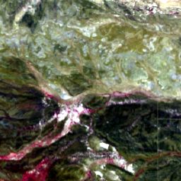
You can also read