Geospatial Analytics for COVID-19 Active Case Detection
←
→
Page content transcription
If your browser does not render page correctly, please read the page content below
Computers, Materials & Continua                                                            Tech Science Press
DOI:10.32604/cmc.2021.013327
Article

              Geospatial Analytics for COVID-19 Active Case Detection
          Choo-Yee Ting1, * , Helmi Zakariah2 , Fadzilah Kamaludin2, Darryl Lin-Wei Cheng1 ,
                                Nicholas Yu-Zhe Tan1 and Hui-Jia Yee2

                                 1
                                   Multimedia University, Cyberjaya, 63100, Malaysia
                           2
                            AIME Healthcare Sdn Bhd, Kuala Lumpur, 59200, Malaysia
                        *
                          Corresponding Author: Choo-Yee Ting. Email: cyting@mmu.edu.my
                               Received: 02 August 2020; Accepted: 12 November 2020

                 Abstract: Ever since the COVID-19 pandemic started in Wuhan, China, much
                 research work has been focusing on the clinical aspect of SARS-CoV-2.
                 Researchers have been leveraging on various Artificial Intelligence techniques
                 as an alternative to medical approach in understanding the virus. Limited stud-
                 ies have, however, reported on COVID-19 transmission pattern analysis, and
                 using geography features for prediction of potential outbreak sites. Predicting
                 the next most probable outbreak site is crucial, particularly for optimizing the
                 planning of medical personnel and supply resources. To tackle the challenge,
                 this work proposed distance-based similarity measures to predict the next most
                 probable outbreak site together with its magnitude, when would the outbreak
                 likely to happen and the duration of the outbreak. The work began with
                 preprocessing of 1365 patient records from six districts in the most populated
                 state named Selangor in Malaysia. The dataset was then aggregated with
                 population density information and human elicited geography features that
                 might promote the transmission of COVID-19. Empirical findings indicated
                 that the proposed unified decision-making approach outperformed individual
                 distance metric in predicting the total cases, next outbreak location, and the
                 time interval between start dates of two similar sites. Such findings provided
                 valuable insights for policymakers to perform Active Case Detection.

                 Keywords: COVID-19; geospatial analytics; active case detection

1 Introduction
    The world is currently experiencing COVID-19 pandemic, which had started at Wuhan, China
in December 2019. Despite the reduction in daily confirmed cases in China, outside of China has
shown a drastic increase in daily confirmed cases. Countries like the United States, Brazil, and
India recorded a daily increase of more than 10000 confirmed cases [1].
     In South-East Asia, Malaysia had experienced its first three COVID-19 confirmed cases on
25 January 2020 [2]. Subsequent cases were reported, and many of them were imported cases,
including those from China and the United States [3]. In late February, the number of COVID-19
confirmed cases increased when there were Malaysians who travelled back from China during that

                     This work is licensed under a Creative Commons Attribution 4.0 International License,
                     which permits unrestricted use, distribution, and reproduction in any medium, provided
                     the original work is properly cited.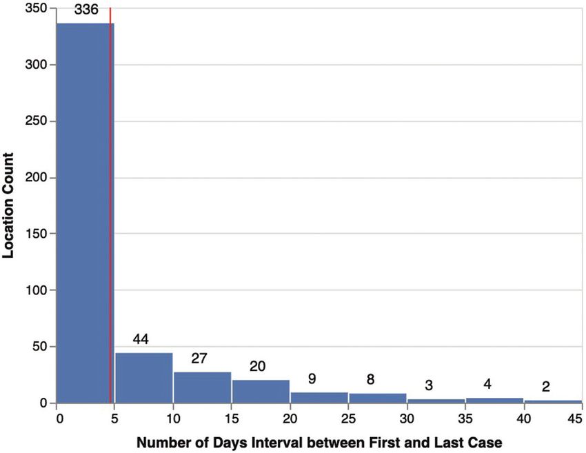
836                                                                             CMC, 2021, vol.67, no.1

time. In March 2020, the Tabligh event that had involved almost 12000 participants was then
resorted to the high daily growth rate in Malaysia, particularly in the state of Selangor [4]. Due to
the exponential growth in confirmed cases, Movement Control Order (MCO) was introduced on
18 March 2020, which was later extended to its 2nd phase on 1 April 2020 and 3rd phase on
15 April 2020 and subsequently entered into its 4th phase of MCO which ends on 12 May
2020 [5]. Currently, Malaysia is in its Recovery MCO (RMCO) until 31 August 2020. During the
two MCOs, both the federal and state governments have implemented various interventions to
prevent a further outbreak by identifying close contacts and conducting mass testing for Active
Case Detection (ACD). MCO is a measure to keep the healthcare system from being overwhelmed
by “flattening the curve” [6] and to minimize the negative impact to all economic sectors caused
by the prolong MCO. One of the many approaches initiated by the Selangor state government
was to deploy geospatial analytics to identify the next most probable areas with an outbreak and
estimate the magnitudes.
     Geospatial analytics has been employed to tackle challenges in site selection for various busi-
ness domains. This has included the retail business [7–12], real-estate [13], public safety [14], disas-
ter monitoring and prevention [12], government [14], planetary [15], agriculture [16], and renewal
energy [17,18]. Researchers have employed different machine learning methods in geospatial ana-
lytics. One of the most common methods that incorporate human knowledge is through Analytical
Hierarchical Technique [18–22]. Other researchers employed Decision Support Systems [23] and
Fuzzy Logic [24].
    Researchers have recently attempted Geographic Information Systems (GIS) for tackling
challenges related to COVID-19 and utilization of Big Data to provide insights in decision-
making [25–27]. Another recent study by Mollalo and colleagues highlighted the use of GIS in
modelling the incident and spread of COVID19 in the United States [28]. The utilization of GIS
has also been reported in Iran, where epidemiological maps of cases were developed to monitor
the incident locations and rates. In Malaysia, geospatial analytics has been deployed for Active
Case Detection (ACD) in late April 2020 in Selangor, Malaysia. However, successful ACD requires
tackling the following challenges:
    (i) how to identify the next most probable outbreak sites (i.e., residential areas)?
   (ii) how to estimate the magnitude of COVID-19 cases for a particular site (i.e.,
        residential area)?
  (iii) what is the time interval between the current and the subsequent case, given two similar
        sites (i.e., residential area)?
     In this paper, the discussion has focused on COVID-19 outbreak that happened at a resi-
dential area, and therefore the “site” refers residential area. Tackling the above challenges began
with gathering, preprocessing and transformation of raw datasets (see Section 3) into an analytical
dataset (see Section 4.1) before different distance metrics can be applied. A detailed discus-
sion about the raw datasets and their transformation can be found in Section 4. In Section 5,
findings of different distance metrics together with their comparison with the proposed unified
decision-making mechanism will be reported.

2 Distance Measure Metrics
    A similarity or dissimilarity measure is a real-valued function that quantifies the similarity
between two items, which in this context refer to records in a database. There are various similarity
measure techniques proposed by researchers [29], and they can be categorized into (i) distance-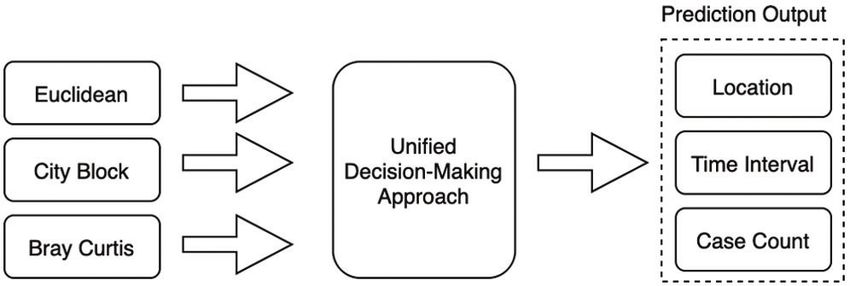
CMC, 2021, vol.67, no.1                                                                             837

based similarity measure, (ii) feature-based similarity measure, and (iii) probabilistic similarity
measure. Among the three techniques, the distance-based similarity measure metric remains most
commonly applied in both the academic and commercial settings. A proper distance requires a
function d to follow the following properties:
     (i)   positivity: d(x, y) ≥ 0
    (ii)   symmetry: d(x, y) = d(y, x)
   (iii)   identity-discerning: d(x, y) = 0, ∴ x = y
   (iv)    triangle inequality: d(x, z) ≤ d(x, y) + d(y, z)
     The commonly applied point-based distance measures are the Euclidean distance, City Block
distance, and Bray Curtis [30]. Both Euclidean distance and City Block are a special case of the
Minkowski family [31–34]. The Minkowski distance can be defined by
              n             1/m

dminkowski =     |xi − yi |m
                                  , m≥1                                                      (1)
                  i=1

where m is a positive real number while xi and yi are two vectors in n-dimension space. By
instantiating m = 1, Eq. (1) is modified to take new form as shown below, and it is known as the
City Block distance (also referred to as the Manhattan distance). The distance between two items is
the sum of the differences of their corresponding components. The City Block distance fulfils the
positivity property in which it is always greater than or equal to zero, as well as identity-discerning
property where the measurement would be high for points that show dissimilarity and zero for
identical points.

               n
dcityblock =         |xi − yi |                                                                      (2)
               i=1

     When Eq. (1) is instantiated by m = 2, the Euclidean distance can then be defined by
              n             1/2

deuclidean =     |xi − yi |2                                                                         (3)
                 i=1

     Euclidean inherited the characteristics of Minkowski, and therefore with the existence of large-
scale continuous values, the large-scale attributes would dominate the others [35–37]. To overcome
such challenges, researchers introduced normalization of continuous features as a solution to the
issue [36]. By introducing the coefficient 1/2 the output of Euclidean distance is scaled down
(normalized) so that a comparison between two points can be accurately presented. Researchers
had proposed an improved version of Euclidean distance such as the Weighted Euclidean [38]. It
is employed to overcome the large-scale attribute issue by the Euclidean distance (Eq. 2), which
incorporates feature weights w1 , w2 , w3 , . . . , wn on each dimension. While having different weights
is crucial, redundant weight assignment could dominate the similarity between data points [39].
Due to incomplete information about influence of geography characteristics towards COVID-19,
this study firstly normalized the continuous data before applying Euclidean distance metric.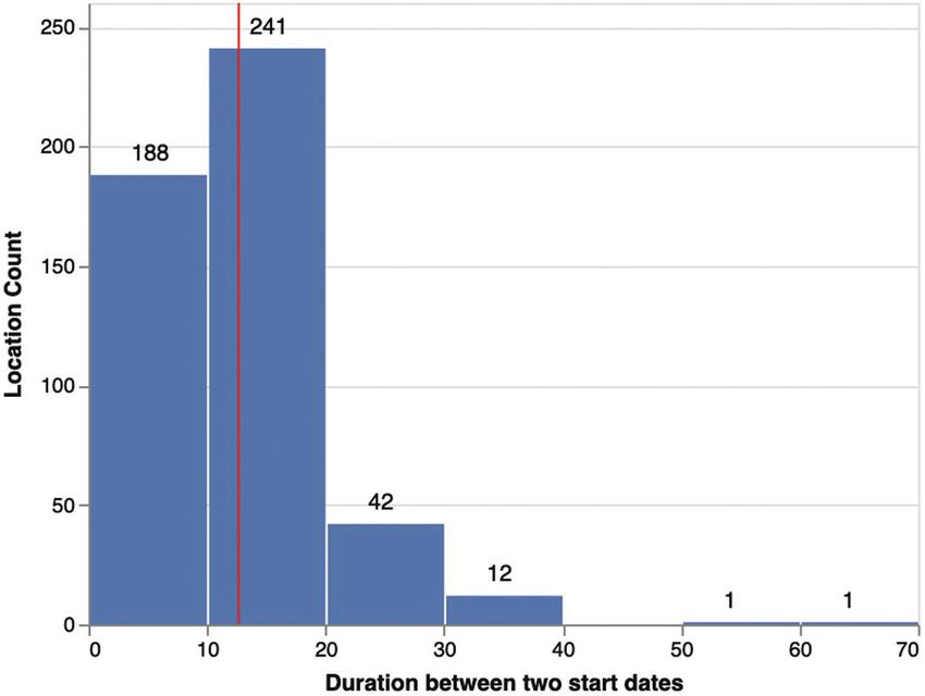
838                                                                          CMC, 2021, vol.67, no.1

     Bray Curtis distance measure [30] quantifies the difference between two samples. The dissimi-
larity is computed on the raw sum of each sample and the sum of differences between the features
of each sample. Similarity can be obtained if the distance or dissimilarity is subtracted by 100.

                |xi − xj |
dbraycurtis =                                                                                 (4)
                |xi + xj |

    In this study, only point-based distance metrics were considered. This is because the number
of variables that formed the analytical dataset is fixed, and the distance (magnitude) between two
points is crucial for prediction work to addresses the challenges successfully.

3 Raw Dataset
    This section begins with a discussion about the raw datasets and the relevant transforma-
tion process to form an analytical dataset. Subsequently, the discussion will be centred around
the implementation of different distance metrics onto the analytical dataset to answer the
research questions.
     Tab. 1 shows the different datasets used in this research work. The first dataset, De , consists
of 1365 patient addresses, with many of them incomplete addresses [40]. The second dataset, Dpop ,
consists of raw population density about children under five, elderly over 60, men, woman, women of
reproductive age, and youth [41]. Preprocessing on the raw dataset was needed because the dataset
provides only population density estimation at the level of individual latitude and longitude. In
this study, the population density was calculated using 500 m radius for each patient location.

                                   Table 1: Dataset information
Dataset                          Description                                                  Source
Patient address (De )            A list of 1365 patient addresses. Many of the                 [40]
                                 addresses are incomplete
Population density (Dpop )       Population density for children under five, elderly           [41]
                                 over 60, men, woman, women of reproductive
                                 age, youth
Residential area (Dres )         A list of residential areas in the state of Selangor,        [42,43]
                                 totalling up to 3374 residential areas as of
                                 2019-10-01.
Point of interest (Dpoi )        A list of 22 categories of point of interest relevant        [44]
                                 to COVID-19 as suggested by epidemiologists
Daily cases (Dcase )             Daily COVID-19 confirmed cases from 2020-02-03               [40]
                                 to 2020-04-23

    The third dataset, Dres , consists of 3374 residential areas in the Selangor state. It originated
from the Valuation and Property Services Department Malaysia [42] and has been digitized by
Brickz.my [43]. The purpose is to detect the names and types of residential area the patients live.
    The fourth dataset, Dpoi , comprises most of the points of interest(POI) in the Selangor state.
The dataset was subscribed from Telekom Malaysia [44], and it has 116402 POI grouped into
1116 categories. Examples of POI are Burger King, KFC, McDonald, Ace Hardware, Starbucks, Ikea,
Parkson, and many more. In the dataset, each point of interest is tagged to a particular category.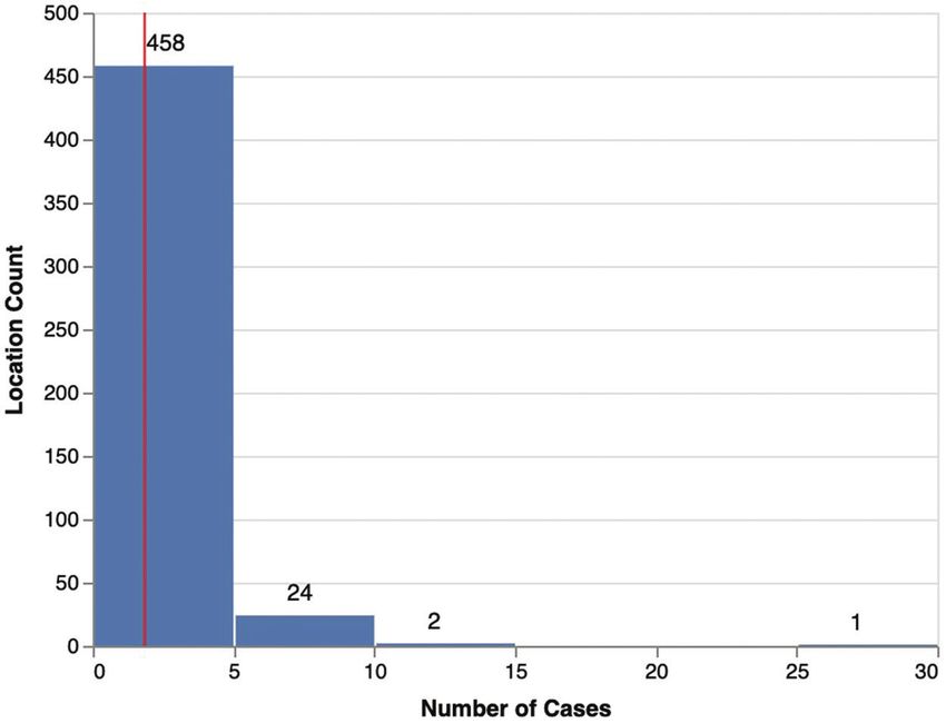
CMC, 2021, vol.67, no.1                                                                          839

Examples of the category are Food & Beverages, Convenient Store, Wet Market, Hardware Store,
Hypermarket, and many more.
     Dcase contains daily COVID-19 confirmed cases in Selangor from 2020-03-03 to 2020-04-
23. The daily cases were transformed into weekly cumulative cases to reflect the SARS-CoV-2
virus incubation period of 5.6 to 7.7 days at 95% CI [45]. Therefore, a 7-day monitoring period
is proposed.

4 Method
    The raw dataset discussed in Section 3 does not allow distance metrics to be applied directly
as well as addressing the research challenges. Therefore, preprocessing and transformation are
prerequisite to constructing an analytical dataset that fits the distance metrics. The subsections
below aim to provide a high-level process from the construction of analytical dataset to proposal
of distance metric utilization. The final subsection highlight the proposal of a unified modelling
approach to avoid bias in a recommendation when relying merely on one distance metric.

4.1 Construction of Analytical Dataset
    A well-designed data structure for the analytical dataset can lead to success in addressing
the research challenges. However, identifying the right variables for the analytical dataset is a
non-trivial task. One of the difficulty is to identify the right points of interest (POI) and their
categories. In this study, two epidemiologists had been consulted to identify POI categories that
are likely to affect COVID-19 transmission. The categories are Agriculture-based trading com-
panies, ATM, Bazaar, Convenient Shop, F&B, Government Health Center, Hardware shops, Higher
Education Institution, Hypermarket, Islamic School, Medical Services, Mini Market, Pharmacy, Shop,
Shopping Complex, Supermarket, Toll, Trading Food, Transport, 24-Hour Shores, Wet Market, and
Whole Sale Market. In total, 22 categories were identified to be included as part of the analytical
dataset (D22
           poi ).

                          Table 2: Analytical dataset with partial features

Patient     Elderly       Children   ...   Start      Convenient Place of       ...   Week_1
address     over 60       under 5          date       store      worship              cases
LocA        321           470        ...   01/3/20    6            3            ...   4           ...
LocB        398           550        ...   15/3/20    11           4            ...   5           ...
...         ...           ...        ...   ...        ...          ...          ...   ...         ...

    Apart from the subsetted POI dataset (D22 poi), the analytical dataset, Danalytics , was formed
by aggregating De , Dpop , Dres , and Dcase . The columns in Tab. 2 are formed by concatenating all
the variables from the datasets. The final analytical dataset consists of 111 variables and captures
mostly numerical values except for the columns “Residential Area” and “Start Date.” Tab. 2 shows
the partial analytical dataset with each record representing a patient’s details. The first record in
Tab. 2 for instance, there is a patient who lives in LocA and within 500 m there are 321 elderly
people with age more than 60, six convenient stores, and three places of worship. The first case
at LocA was reported on 1 March 2020. The second record in the table shows a patient who lives
at LocB , which is having higher population density and more POI as compared to LocA . The first
case reported at LocB was 15 March 2020, which is two weeks after LocA had its first case. In
840 CMC, 2021, vol.67, no.1
this study, place of worship is one of the crucial variable because in Selangor, a major COVID-19
outbreak happened after the Tabligh event ended in middle of March 2020 [4].
4.2 Measuring the Similarity Between Sites
The construction of analytical dataset has led to the design of algorithms that utilizes the
distance metrics to tackle the research questions. There are two algorithms designed, with the
first identifying top-3 most similar locations to a location of interest. The second algorithm
estimates the time interval and total cases for the next most probable locations with at least one
COVID-19 case.
Algorithm 1 was proposed to tackle the first research challenge in which it predicts the next
most prob-able location with at least a confirmed case. The input to the algorithm is the analytical
dataset, Danalytics , the distance metrics where metric ∈ {Euclidean, City Block, Bray Curtis}, and a
location of interest L. As shown in the algorithm, the location of interest is measured against
L
all locations in the analytical dataset to elicit its respective similarity scores (Smetric ). This can
be performed via the function metric—Similarity—Loc( ). The output of the algorithm is a
top3(L)
dataset, Dmetric , which contains locations with the three highest similarity scores for L.
top3(L)
The output of Algorithm 1, Dmetric , is fed into Algorithm 2 to estimate the mean duration
for L to observe its first case. This is performed through the function dayDiff-mean( ) which
calculates the mean of time interval for L’s similar locations that had demonstrated at least one
case. The algorithm also estimates of mean total cases through the function case-mean( ).
4.3 Decision-Making Strategy
The three different distance metrics produce different distance scores and the top-3 locations.
Relying solely on one distance metric for decision-making can be risky and bias. Therefore, this
study proposed a unified approach to decision-making by calculating the mean value from the
output of the three different distance metrics. The high-level process flow is shown in Fig. 1, while
the detailed steps are shown in Algorithm 3.CMC, 2021, vol.67, no.1 841
Figure 1: Decision-making strategy
Algorithm 3 discusses the procedure to aggregate the scores are given by different distance-
based similarity measure techniques. To normalize the bias inherent within the metrics, inner-
join was performed on the output of Algorithm 1 generated using different metrics. The
aggregated dataset was then fed into two functions, namely calc-caseCount-mean( ) and
L ) and the day
calc-dayDiff-mean( ) to produce the final prediction on the total cases (Cfinal
interval for that particular location of interest to have its first case (tL
final ).
5 Empirical Findings
5.1 Statistical Overview of Dataset
This section begins with a statistical overview of the dataset used in this study. Histograms are
generated based on the following criteria: (i) sites (i.e., residential areas) and total cases, (ii) day
interval between the first and last case of a site, (iii) day difference for start dates of two similar
site, (iv) average similarity score between a site and its three most similar sites.
Fig. 2 shows that most of the residential areas in the Selangor state had experienced 5 cases
and below, totalling up to 458 locations. There were 24 residential areas with cases between 5 and
10. There was only one location with more than 25 cases.
As shown in Fig. 3, there were 336 resident areas had their first and last cases within an
interval of 5 days. From the raw dataset, most of the residential areas had either 1 or 2 cases only
within 5 days period. Those residential areas that had more than 15 days interval contributed to
10.15% of the total residential areas.
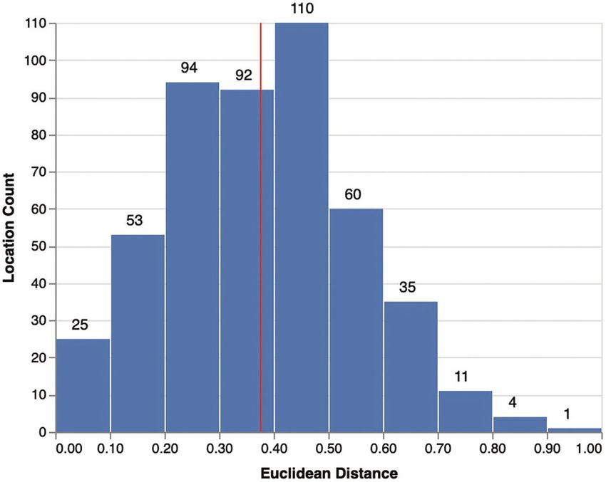
The graph above shows the average distance scores between any one residential area and its
top-3 similar ones (Fig. 4). When calculated via Euclidean distance, most of the residential areas
depicted the distance less than 0.5, indicating that there are common characteristics among the
residential areas in the Selangor state. To be specific, there are 77.1% of residential areas with
average distance scores less than 0.5.842 CMC, 2021, vol.67, no.1
Figure 2: Residential areas with different number of cases
Figure 3: Day intervals between the first and last case
Fig. 5 shows the distribution of duration between the start dates of two residential areas. It
was found that in average the time interval between any two similar residential areas was 12 days.
In other words, for any two similar residential areas, the latter residential area will likely to observe
a case after a case was observed a area similar to it. However, low possibility could be observedCMC, 2021, vol.67, no.1 843
for any two similar residential area to have a large time interval. This is shown in the figure that
only one location with a time interval of more than 60 days.
Figure 4: Average distance score between a residential area with its top-3 similar areas
Figure 5: Average duration between 2 start dates844 CMC, 2021, vol.67, no.1
5.2 Performance of Distance Metrics
5.2.1 Prediction of Total Cases
In this study, a total of 532 records were used for evaluation of the performance of the
top3(L) top3(L)
three distance metrics. These records were selected because they appeared in Deu , Dbc ,
top3(L)
and Dcb .
The predicted total cases were benchmarked against the actual total cases, and the
evaluation metrics are Mean Absolute Error (MAE), Mean Square Error (MSE), and Root Mean
Square Error (RMSE). As shown in Tab. 3, the results showed that Euclidean outperformed Bray
Curtis and City Block in predicting the total case using MAE, however, the Unified Modeling
approach outperformed the rest when MSE and RMSE were used.
Table 3: Total case prediction by three difference evaluation metrics and proposed a unified
decision-making approach
MAE MSE RMSE
Euclidean 6.7105 74.3157 8.6206
Bray curtis 7.1390 77.7706 8.8187
City Block 6.8872 81.8571 9.0474
Unified decision-making 6.7431 71.0797 8.4308
5.2.2 Outbreak Duration Prediction
Tab. 4 shows the prediction of duration between the first and last case in a particular
residential area.
Comparing among the three distance measure techniques, Euclidean outperformed Bray Curtis
and City Block for all three evaluation metrics. Comparing to the prediction of total cases,
the Unified Modeling approach consistently depicted the lowest error rates in the prediction of
duration between the first and last case when MAE, MSE, and RMSE was used.
Table 4: Prediction of outbreak duration
MAE MSE RMSE
Euclidean 5.1303 54.9494 7.4127
Bray Curtis 5.1478 56.6946 7.5295
City block 5.1234 63.2988 7.9560
Unified decision-making 5.0490 54.5591 7.3864
Table 5: Difference in two start dates
MAE MSE RMSE
Euclidean 5.5344 46.3068 6.8049
Bray Curtis 5.5764 46.9360 6.8509
City block 5.6347 49.5900 7.0420
Unified decision-making 5.3842 43.4475 6.5914CMC, 2021, vol.67, no.1 845
5.2.3 Day Interval Between Start Dates of Two Similar Sites
One of the challenges in this research work was to predict the duration between the start
dates of two similar residential areas. This would allow medical resources to be planned and
optimized in the event that a COVID-19 patient is detected at a particular residential area.
The proposed algorithms were able to predict the day intervals between a former and a latter
residential area. Based on the experiment findings shown in Tab. 5, the Unified Decision-Making
approach, had again, outperformed Bray Curtis, Euclidean, and City Block with 5.3842, 43.4475,
and 6.5914, respectively.
6 Conclusion
Although there has not been a conclusive study of the SARS-CoV-2 virus that is causing the
COVID19 pandemic now, it has generally been characterized by having high infectious rate and
having varying incubation period. More worrying is when there are patients that are reported to be
asymptomatic. Such characteristics have together explained the rapid development of an epidemic
in Malaysia and worldwide. While waiting for the vaccine to be developed, one of the solutions
to minimize outbreak is via active monitoring and mass screening. Performing mass screening
can be taxing in both human and medical resources. A possible solution to the challenge is by
deploying geospatial analytics. The research work presented in this paper attempt to answer the
following questions: (i) how to identify the site (residential areas) where COVID-19 cases may
appear next? (ii) what is the estimate of COVID-19 cases for that new residential area? (iii) what
is the time interval before a COVID-19 case is observed at a similar residential area? Answering
the questions require relevant datasets. Four different datasets were identified, and they are the
patient addresses, population density, residential areas, daily cases, and point of interest. These
datasets were transformed into an analytical dataset before feeding into distance-based similarity
measure metrics.
In this study, three distance-based similarity measures had been employed in this study
to measure the distance (a.k.a similarity) between two records. The distance metrics used are
Euclidean distance, City Block distance, and Bray Curtis distance. Rather than relying on the results
elicited by one distance metric, an unified modelling approach, which takes the average of 3
output, was proposed. The empirical findings suggested that the unified modelling approach is a
promising approach to tackle the challenges listed above. The proposed approach outperformed
any single distance metric such as Euclidean, City Block, and Bray Curtis in almost all the
evaluation metrics, which have included the MAE, MSE, and RMSE. It is therefore suggesting
that the Unified Decision-Making approach to similarity measures can be a solution to effective
monitoring and proactive intervention.
The work can be extended to three perspectives. First is to deploy other types of distance
metrics such as cosine distance, average distance, and weighted Euclidean. Second, the study could
deploy machine learning approach such as classification and clustering to predict the total case
and duration of an outbreak at a particular zone. Third, this research work has listed 22 categories
of Point of Interest relevant to COVID-19 transmission. Further work could be done to rank the
categories according to their importance towards influencing COVID-19 transmission.
Acknowledgement: The authors thank the Government of Selangor to provide partial COVID-19
patient information for the purpose of academic use.846 CMC, 2021, vol.67, no.1
Funding Statement: The authors received no specific funding for this study.
Conflicts of Interest: The authors declare that they have no conflicts of interest to report regarding
the present study.
References
[1] WHO, “Novel coronavirus (2019-ncov) situation reports,” 2020. [Online]. Available: https://www.who.
int/emergencies/diseases/novel-coronavirus-2019/situation-reports.
[2] Reuters, “Malaysia confirms first cases of coronavirus infection,” 2020. [Online]. Available:
https://www.reuters.com/article/china-health-malaysia/malaysia-confirms-first-cases-of-coronavirus-
infection-idUSL4N29U03A.
[3] Theedgemarketscom, “Three covid-19 cases confirmed in malaysia today, bringing total to 22,” 2020.
[Online]. Available: https://www.theedgemarkets.com/article/ two-new-confirmed-covid19-cases-malaysia.
[4] T. Sukumaran, “How the coronavirus spread at malaysia’s tabligh islamic gathering,” 2020. [Online].
Available: https://www.scmp.com/week-asia/explained/article/3075968/how-coronavirus-spread-malaysias-
tabligh-islamic-gathering.
[5] F. M. Today, “Mco extended 2 weeks to may 12,” 2020. [Online]. Available: https://www.
freemalaysiatoday.com/category/nation/2020/04/23/mco-extended-2-weeks-to-may-12/.
[6] J. C. McGinty, “What will it take to flatten the coronavirus curve?,” 2020. [Online]. Available:
https://www.wsj.com/articles/what-does-it-mean-to-flatten-the-curve-to-fight-coronavirus-11585301402.
[7] K. L. Ailawadi and P. W. Farris, “Managing multi- and omni-channel distribution: Metrics and research
directions,” Journal of Retailing, vol. 93, no. 1, pp. 120–135, 2017.
[8] E. T. Bradlow, M. Gangwar, P. Kopalle and S. Voleti, “The role of big data and predictive analytics
in retailing,” Journal of Retailing, vol. 93, no. 1, pp. 79–95, 2017.
[9] M. G. Dekimpe, “Retailing and retailing research in the age of big data analytics,” International Journal
of Research in Marketing, vol. 37, no. 1, pp. 3–14, 2020.
[10] D. Grewal, A. L. Roggeveen and J. Nordfalt, “The future of retailing,” Journal of Retailing, vol. 93,
no. 1, pp. 1–6, 2017.
[11] Y. Liu, H. Wang, G. Li, J. Gao, H. Hu et al., “ELAN: An efficient location-aware analytics system,”
Big Data Research, vol. 5, pp. 16–21, 2016.
[12] A. Trivedi and A. Singh, “A hybrid multi-objective decision model for emergency shelter location-
relocation projects using fuzzy analytic hierarchy process and goal programming approach,” Interna-
tional Journal of Project Management, vol. 35, no. 5, pp. 827– 840, 2017.
[13] M. Lukas and E. López-Morales, “Real estate production, geographies of mobility and spatial con-
testation: A two-case study in santiago de chile,” Journal of Transport Geography, vol. 67, pp. 92–101,
2018.
[14] J. Wang, C.-H. Tsai and P.-C. Lin, “Applying spatial-temporal analysis and retail location theory
to public bikes site selection in taipei,” Transportation Research Part A: Policy and Practice, vol. 94,
pp. 45–61, 2016.
[15] P. Cui, D. Ge and A. Gao, “Optimal landing site selection based on safety index during planetary
descent,” Acta Astronautica, vol. 132, pp. 326–336, 2017.
[16] M. Chavez, P. Berentsen and A. O. Lansink, “Assessment of criteria and farming activities for tobacco
diversification using the analytical hierarchical process (ahp) technique,” Agricultural Systems, vol. 111,
pp. 53–62, 2012.
[17] M. Shaheen and M. Z. Khan, “A method of data mining for selection of site for wind turbines,”
Renewable and Sustainable Energy Reviews, vol. 55, pp. 1225–1233, 2016.
[18] M. Vasileiou, E. Loukogeorgaki and D. G. Vagiona, “GIS-based multi-criteria decision analysis for
site selection of hybrid offshore wind and wave energy systems in Greece,” Renewable and Sustainable
Energy Reviews, vol. 73, pp. 745–757, 2017.CMC, 2021, vol.67, no.1 847
[19] J. Garcia, A. Alvarado, J. Blanco, E. Jimenez, A. Maldonado et al., “Multi-attribute evaluation
and selection of sites for agricultural product warehouses based on an analytic hierarchy process,”
Computers and Electronics in Agriculture, vol. 100, pp. 60–69, 2014.
[20] T. Sahin, S. Ocak and M. Top, “Analytic hierarchy process for hospital site selection,” Health Policy
and Technology, vol. 8, no. 1, pp. 42–50, 2019.
[21] A. A. Merrouni, F. E. Elalaoui, A. Mezrhab, A. Mezrhab and A. Ghennioui, “Large scale pv sites
selection by combining gis and analytical hierarchy process. Case study: Eastern morocco,” Renewable
Energy, vol. 119, pp. 863–873, 2018.
[22] M. Fabjanowicz, M. Bystrzanowska, J. Namiesnik, M. Tobiszewski and J. Plotka-Wasylka, “An ana-
lytical hierarchy process for selection of the optimal procedure for resveratrol determination in wine
samples,” Microchemical Journal, vol. 142, pp. 126–134, 2018.
[23] C. Eastwood, D. Chapman and M. Paine, “Networks of practice for co-construction of agricultural
decision support systems: Case studies of precision dairy farms in Australia,” Agricultural Systems,
vol. 108, pp. 10–18, 2012.
[24] A. Y. Topraklı, A. Adem and M. Dagdeviren, “A courthouse site selection method using hesitant fuzzy
linguistic term set: A case study for turkey,” Procedia Computer Science, vol. 102, pp. 603–610, 2016.
[25] C. Zhou, F. Su, T. Pei, A. Zhang, Y. Du et al., “Covid-19: Challenges to GIS with big data,” Geography
and Sustainability, vol. 1, no. 1, pp. 77–87, 2020.
[26] Z. Arab-Mazar, R. Sah, A. A. Rabaan, K. Dhama and A. J. Rodriguez-Morales, “Mapping the
incidence of the covid-19 hotspot in iran implications for travellers,” Travel Medicine and Infectious
Disease, vol. 34, pp. 101630, 2020.
[27] M. Lewin, “How better location intelligence can help businesses cope with covid-19_2020,” 2020.
[Online]. Available: https://resources.esri.ca/news-and-updates/how-better-location-intelligence-can-help-
businesses-cope-with-covid-19.
[28] A. Mollalo, B. Vahedi and K. M. Rivera, “GIS-based spatial modeling of covid-19 incidence rate in
the continental united states,” Science of the Total Environment, vol. 728, pp. 138884, 2020.
[29] F. G. Ashby and D. M. Ennis, “Similarity measures,” 2020. [Online]. Available:
http://www.scholarpedia.org/.
[30] J. R. Bray and J. T. Curtis, “An ordination of the upland forest communities of southern wisconsin,”
Ecological Monographs, vol. 27, no. 4, pp. 325–349, 1957.
[31] J. Dattorro, Convex optimization & euclidean distance geometry. USA: Meboo Publishing, 2005.
[32] J. Gower, “Euclidean distance geometry,” Mathematical Scientist, vol. 7, no. 1, pp. 1–14, 1982.
[33] J. Han, M. Kamber and J. Pei, Data mining concepts and techniques. 3rd ed., Waltham, Mass: Morgan
Kaufmann Publishers, 2012.
[34] S.-H. Cha, “Comprehensive survey on distance/similarity measures between probability density func-
tions,” City, vol. 1, no. 2, pp. 1, 2017.
[35] A. S. Shirkhorshidi, S. Aghabozorgi and T. Y. Wah, “A comparison study on similarity and dissimilarity
measures in clustering continuous data,” PLoS ONE, vol. 10, no. 12, pp. e0144059, 2015.
[36] A. K. Jain, M. N. Murty and P. J. Flynn, “Data clustering: A review,” ACM Computing Surveys, vol. 31,
no. 3, pp. 264–323, 1999.
[37] J. Mao and A. K. Jain, “A self-organizing network for hyperellipsoidal clustering (hec),” IEEE
Transactions on Neural Networks, vol. 7, no. 1, pp. 16–29, 1996.
[38] R. V. Rao, D. Singh, F. Bleicher and C. Dorn, “Weighted euclidean distance-based approach as
a multiple attribute decision making method for manufacturing situations,” International Journal of
Multicriteria Decision Making, vol. 2, no. 3, pp. 225–240, 2012.
[39] D. Hand, P. Smyth and H. Mannila, Principles of Data Mining. Cambridge, Massachusetts, USA: MIT
Press, 2001.
[40] S. Government, “Dasar keselamatan ict,” 2020. [Online]. Available: https://www.selangor.gov.my/.848 CMC, 2021, vol.67, no.1
[41] HDX. Malaysia, “High resolution population density maps + demographic estimates,” 2020.
[Online]. Available: https://data.humdata.org/dataset/malaysia-high-resolution-population-density-maps-
demographic-estimates.
[42] JPPH, “Valuation and property services department Malaysia,” 2020. [Online]. Available:
https://www.jpph.gov.my/v3/ms/.
[43] Brickz, Brickz, “True property prices,” 2020. [Online]. Available: https://www.brickz.my/.
[44] T. Malaysia, “Telekom malaysia,” 2020. [Online]. Available: https://www.tm.com.my/Pages/Home.aspx,
Accessed: 2020-04-27.
[45] S. A. Lauer, K. H. Grantz, Q. Bi, F. K. Jones, Q. Zheng et al., “The incubation period of coronavirus
disease 2019 (covid-19) from publicly reported confirmed cases: Estimation and application,” Annals of
Internal Medicine, vol. 172, no. 9, pp. 577–582, 2020.You can also read


