Globalemu: A novel and robust approach for emulating the sky-averaged 21-cm signal from the cosmic dawn and epoch of reionisation

MNRAS 000, 1–11 (2021) Preprint 12 April 2021 Compiled using MNRAS LATEX style file v3.0

 globalemu: A novel and robust approach for emulating the sky-averaged
 21-cm signal from the cosmic dawn and epoch of reionisation
 H. T. J. Bevins,1★ W. J. Handley,1,2 A. Fialkov,2,3 E. de Lera Acedo1,2 and K. Javid1,2
 1 Astrophysics Group, Cavendish Laboratory, J. J. Thomson Avenue, Cambridge, CB3 0HE, UK
 2 Kavli Institute for Cosmology, Madingley Road, Cambridge CB3 0HA, UK
 3 Institute of Astronomy, University of Cambridge, Madingley Road, Cambridge CB3 0HA, UK
arXiv:2104.04336v1 [astro-ph.CO] 9 Apr 2021

 Accepted XXX. Received YYY; in original form ZZZ

 ABSTRACT
 Emulation of the Global (sky-averaged) 21-cm signal from the Cosmic Dawn and Epoch of Reionization with neural networks
 has been shown to be an essential tool for physical signal modelling. In this paper we present globalemu, a Global 21-cm signal
 emulator that uses redshift as a character defining variable along side a set of astrophysical parameters to estimate the brightness
 temperature of the 21-cm signal. Combined with a physically motivated pre-processing of the data this makes for a reliable
 and fast emulator that is relatively insensitive to the neural network design. A single high resolution signal can be emulated in
 1.3 ms when using globalemu in comparison to 133 ms, a factor of 102 improvement, when using the existing public state of
 the art emulator 21cmGEM evaluated with the same computing power. We illustrate, with the same training and test data used
 for 21cmGEM, that globalemu is almost twice as accurate as 21cmGEM and for 95% of models in a test set of ≈ 1, 700 we can
 achieve a of ≤ 5.37 mK and a mean of 2.52 mK across the band = 7 − 28 (approximately 10% the expected
 noise of 25 mK for the Radio Experiment for the Analysis of Cosmic Hydrogen (REACH)). Further, globalemu provides a
 flexible framework in which the neutral fraction history and Global signal models with updated astrophysics can be emulated
 easily. The emulator is pip installable and available at: https://github.com/htjb/globalemu. globalemu will be used by
 the REACH collaboration to perform physical signal modelling inside a Bayesian nested sampling loop.
 Key words: dark ages – reionization – first stars – early universe – software: data analysis – software: simulations

 1 INTRODUCTION dark-ages-polarimeter-pathfinder/) and MIST (Mapper of
 the IGM Spin Temperature, http://www.physics.mcgill.ca/
 The Global 21-cm signal from the Cosmic Dawn (CD) and Epoch of
 mist/) among others.
 Reionization (EoR), if observed, will provide detailed information
 about the large scale properties of the early universe. The observable The intensity of the signal is measured against the radio back-
 signal is the sky averaged 21-cm emission from the spin flip tran- ground, typically assumed to be equal to the CMB temperature,
 sition in neutral hydrogen at redshifts = 5 − 50 and redshifted to and characterised by an absorption trough and an emission at late
 frequencies of approximately = 50 − 200 MHz. redshifts. The relative magnitude of the signal features is deter-
 An absorption signal was reported at 78 MHz by the Experiment to mined by various astrophysical processes including; the Wouthuysen-
 Detect the Global Epoch of Reionization Signature (EDGES) collab- Field effect (Wouthuysen 1952; Field 1959), Lyman- heating and
 oration in 2018 (Bowman et al. 2018). However, the reported signal CMB heating (Chuzhoy & Shapiro 2007; Venumadhav et al. 2018;
 is significantly larger in amplitude than that predicted by standard Villanueva-Domingo et al. 2020; Mittal & Kulkarni 2020; Reis et al.
 ΛCDM cosmology (Reis et al. 2021) and there are concerns about 2021), X-ray heating and ionization of the hydrogen gas by UV emis-
 the data analysis used (Hills et al. 2018; Singh & Subrahmanyan sion (Madau et al. 1997). A detailed discussion of the physics describ-
 2019; Sims & Pober 2020; Bevins et al. 2021). Efforts are under- ing the Global 21-cm signal can be found in Furlanetto et al. (2006),
 way to make further observations of the signature with a variety of Pritchard & Loeb (2012), Barkana (2016) and Mesinger (2019). The
 different radio telescopes including SARAS (Shaped Antenna mea- physical processes themselves and hence the Global signal can be
 surement of the background RAdio Spectrum, Singh et al. 2018), characterised by a set of astrophysical parameters (see section 3 and
 REACH (Radio Experiment for the Analysis of Cosmic Hydrogen, Cohen et al. (2020)): the star formation efficiency, ∗ , the minimal
 de Lera Acedo 2019), PRIZM (Probing Radio Intensity at High-Z virial circular velocity, , the X-ray efficiency, , the CMB optical
 from Marion, Philip et al. 2019), LEDA (Large-aperture Experiment depth, , the slope of the X-ray spectral energy density (SED), , the
 to Detect the Dark Ages, Price et al. 2018), DAPPER (Dark Ages Po- low energy cut off of the X-ray SED, min , and the mean free path of
 larimeter PathfindER, https://www.colorado.edu/project/ ionizing photons, mfp .
 Hybrid approaches are used to calculate realizations of the 21-cm
 signal, over a large cosmological volume and redshift range, which
 ★ E-mail: htjb2@cam.ac.uk then can be averaged at every redshift separately to give the Global

 © 2021 The Authors

2 H. T. J. Bevins et al.
signal (e.g. Mesinger et al. 2011; Visbal et al. 2012; Fialkov & processing. We provide a demonstration of its accuracy and efficiency
Barkana 2014; Cohen et al. 2017; Reis et al. 2021). Each simulation in this paper using the same data used to train 21cmGEM and the
takes several hours to perform on a desktop (Monsalve et al. 2019) corresponding trained models are publicly available on GitHub. We
and though this is much faster than hydrodynamical simulations this use GitHub actions to perform continuous integration.
time is too long to allow us to constrain astrophysical parameters In section 2 we describe the novel approach used to parameterise
using data. Therefore the desire to emulate the Global signal with globalemu. Section 3 describes the training and test data used to
neural networks, trained on the results of the large scale simulations, illustrate the capabilities of globalemu in this paper and the astro-
has arisen. The neural networks can produce a realisation of the physical parameters in the simulations of the Global signal. We then
Global signal in a fraction of a second by interpolating between describe the predominantly physically motivated pre-processing of
the simulated cosmological and astrophysical models. This means the inputs and outputs of the neural network in section 4. A discussion
they can be used to physically model the signal in, for example, of the neural network structure follows in section 5 and the quality
Bayesian nested sampling loops1 , as in the REACH data analysis of emulation is assessed in section 6. We conclude in section 7.
pipeline (Anstey et al. 2020), in which millions of calculations need
to be made to infer cosmological parameters (Liu & Shaw 2020;
Chatterjee et al. 2021, Sims et al. 2021 (in prep.)).
 21cmGEM is the only existing emulator used to accurately, with
a maximum normalised RMSE of 10.55%, and quickly (see sec-
tion 6.1) emulate the Global 21-cm signal (Cohen et al. 2020). It has
 2 PARAMETERISING THE PROBLEM
previously been used to provide constraints on the parameter space
of the 21-cm signal using EDGES high-band data (Monsalve et al. There are several approaches that can be used to emulate the Global
2019). The emulator uses Principle Component Analysis (PCA, Pear- 21-cm signal with a neural network. The ultimate goal of the emulator
son 1901), the seven astrophysical parameters detailed above and in is to take in a set of astrophysical parameters and return an estimate
section 3, additional information about the mean collapsed fraction of the signal brightness temperature as a function of redshift, ( ),
of halos as a function of redshift, coll ( ), the fraction of X-ray energy where the relationship has been learned from detailed numerical
above 1 keV, XR>1keV , and 2 keV, XR>2keV , and relies on a divi- simulations. This can be done directly with a neural network that
sion of the signal into 2 or 3 distinct segments defined by the turning returns a value of for each redshift data point it has be trained
points. It involves the application of a decision tree for classification on. However, assuming the network is trained on high resolution
and several regression neural networks estimating PCA components, signals this would result in a large number of outputs, making it
the frequencies and temperatures of turning points as well as addi- hard to train, and would be limited in predictive power to specific
tional parameters such as the frequency at which the neutral fraction values of redshift. The process can also be achieved by estimating,
equals 0.16, ( = 0.16). via a neural network, coefficients of a compressed representation of
 In this paper we present globalemu which uses a novel and ro- the signal space. For example, using PCA as with 21cmGEM (Cohen
bust approach with a single small scale neural network to emulate et al. 2020) or learning coefficients of basis functions for polynomials
the Global 21-cm signal given a comprehensive set of astrophysi- or wavelets that when combined return the Global signal. However,
cal parameters and redshift range. Where previously 21cmGEM was whilst this approach reduces the number of outputs compared to a
designed to take in astrophysical parameters and return a low dimen- direct emulation, if incorrectly designed this can result in information
sional representation of the Global signal as a function of redshift, loss and is equally limited in predictive power.
globalemu takes in the same astrophysical parameters and redshift We take the novel approach of using redshift as an input to the
and returns the signal temperature at the corresponding redshift (see network alongside the astrophysical parameters and returning from
Fig. 1). This greatly simplifies the complexity of the relationship the network a single temperature corresponding to the given redshift.
being learnt by the neural network. It means we can achieve accurate This is beneficial for two reasons; the small number of inputs and
results, with the smoothness of the signal imposed by the interpola- outputs means that the network can retain a simple structure and
tion of the neural network between signals in the training data set, second the network will be able to interpolate between the values
using a small network and without the need for a compressed rep- of redshift that it has been trained on. The smooth structure of the
resentation of the signals like PCA where there is a potential loss output from the network is guaranteed by the smooth interpolation
of information. Additionally, globalemu relies on a physically mo- performed by the neural network and by the smooth structure of the
tivated pre-processing of the training data and can emulate a high signals it is learning. Vectorised calls to the network are used to
resolution, = 0.1 over the range = 5 − 50, Global 21-cm signal emulate the temperature as a function of redshift.
in ≈ 1.3 ms. globalemu will be used extensively by the REACH In globalemu we also provide the ability to emulate the evolution
collaboration and has been designed to have an average accuracy less of the neutral fraction, , of hydrogen as a function of redshift.
than or equal to 10% of the expected noise in the REACH system, We use an identical framework as when emulating the Global signal
estimated at 25 mK (REACH Collaboration 2021 (in prep.)). to do this with a set of astrophysical parameters and a redshift as
 globalemu is written in Python using tensorflow and the KERAS inputs to a neural network and a corresponding value of as an
backend, it is pip installable via pip install globalemu and output.
available at https://github.com/htjb/globalemu. It is flexi- We have made efforts to avoid the introduction of "neural network
ble enough to be retrained on any set of Global 21-cm signal mod- magic" into our emulator. We have built a network that can emulate
els whilst maintaing the novel design and physically motivated pre- the Global 21-cm signal to a high degree of accuracy without the need
 for L1 and L2 regularisation, dropout (Srivastava et al. 2014), batch
 normalisation (Ioffe & Szegedy 2015) or other similar concepts. We
1 Note that here we are not referring to a Bayesian Neural Network (see Javid have achieved this by focusing on the pre-processing of the networks
et al. 2020) but rather parameter optimisation algorithms such as polychord inputs and outputs in the desire to set our problem up in a way that
(see Handley et al. 2015a,b). is simple to solve with a basic neural network of a ‘reasonable’ size.

MNRAS 000, 1–11 (2021)

globalemu: Emulating the Global 21-cm signal 3

 21cmGEM globalemu
 x5 or 6 + Decision Tree
 log(f∗ )
 log(Vc )
 log(fX ) log(f∗ )
 τ log(Vc )

 PCA components etc.
 α log(fX )

 Hidden Layers
 νmin τ
 T
 Rmfp α
 f∗ fcoll (20) νmin
 f∗ fX fcoll (15) Rmfp
 ζfcoll (10) z
 fXR>1keV
 fXR>2keV

Figure 1. Left Panel: There currently exists only one other global signal emulator, 21cmGEM, and we provide here an illustration of the regression neural
networks used there. Note that 21cmGEM uses either 5 or 6 of these networks and a decision tree when making predictions. For one of the regression networks
used the only input parameters are the seven astrophysical parameters detailed in section 3 (excluding redshift). However, for the others there is an additional five
derived parameters (see text and Cohen et al. (2020)) and we illustrate the full set of 12 inputs. The number of output nodes depends on the specific application
of the network and they can correspond to either PCA components (4 nodes), additional parameters such as ( = 0.16) (1 node) and the frequencies
and brightness temperatures of turning points in the signal (7 or 5 nodes). The hidden layer in all of the 21cmGEM regression networks has 40 nodes. For a
full illustration of the 21cmGEM algorithm and detailed description see Fig. 11 and section 4.2 in Cohen et al. (2020). Right Panel: An illustration of the
globalemu neural network. Note the use of only one network to emulate the global signal in comparison to the 5 or 6 used for 21cmGEM. Here the input layer
has eight nodes (seven astrophysical parameters plus redshift) and the output layer is a single node returning the brightness temperature corresponding to the
input redshift. We show a sizable hidden layer structure here with the red nodes and ‘...’ however we note that the reduced number of inputs and outputs implies
that a small architecture will be sufficient to achieve a high level of accuracy in the emulation (see section 5).

3 THE TRAINING AND TEST DATA Lyman- flux and late onset of X-ray heating leading to a shallower
 absorption trough and weak or non-existent emission above 0 mK in
In this paper we use the same model signals and corresponding as-
 the signal.
trophysical parameters used to train and test 21cmGEM (available
at https://doi.org/10.5281/zenodo.4541500, Cohen et al. • : The minimal virial circular velocity has a value in the range
2021). Examples of the Global signals from the training set are 4.2 − 100 km/s and is proportional to the cube root of the minimum
shown in Fig. 2. In total the data set contains 27,292 training mod- threshold mass for star formation. A low value of corresponds to
els and 2,174 test models with each model being dependent on 7 a small minimum mass threshold which in turn leads to an earlier
astrophysical parameters. Each Global signal in the data set has 451 onset of Lyman- coupling, responsible for the absorption feature
redshift data points and this means that each signal corresponds to in the Global 21-cm signal, and shifts the minimum of the signal to
451 training points with the same astrophysical parameters and dif- higher redshifts.
ferent redshits. Therefore, for globalemu the 27,292 training mod-
 • : The X-ray efficiency of sources has a range between 0 −
els become 12,308,692 training data points. However, we continue
 1000 and a high value corresponds to a high total X-ray luminosity.
throughout this paper to talk generally of training signals rather than
 This leads to an earlier onset of X-ray heating which also shifts the
data points because the emulator will be used to determine the signal
 minimum of the signal to higher redshifts, contributes to a shallower
structure over a redshift range (see section 6 for more details).
 absorption and results in a significant emission feature during re-
 The data pre-processing is explained in detail in section 4. Explic-
 ionisation at low redshifts.
itly, the inputs (Cohen et al. 2017; Monsalve et al. 2019; Cohen et al.
2020) to the neural network when training on the 21cmGEM data are • : The CMB optical depth in the 21cmGEM data sets takes a
as follows (ranges are based on those in the 21cmGEM training data value in the range 0.04 − 0.2 and a higher value of corresponds to
set, see section 2.5 of Cohen et al. (2020)); a higher value of the ionizing efficiency of sources, . For high we
 would see an earlier reionisation of the hydrogen gas. We note that
 • ∗ : The star formation efficiency takes values in the range is given as 0.054 ± 0.007 by Planck Collaboration VI (2020) and
0.0001 − 0.5 and characterises the amount of gas converted to stars that this falls at the lower end of the range in our training and testing
in the dark matter halos. A low star formation rate results in a low data set. More recent parameter studies have explored lower values

 MNRAS 000, 1–11 (2021)

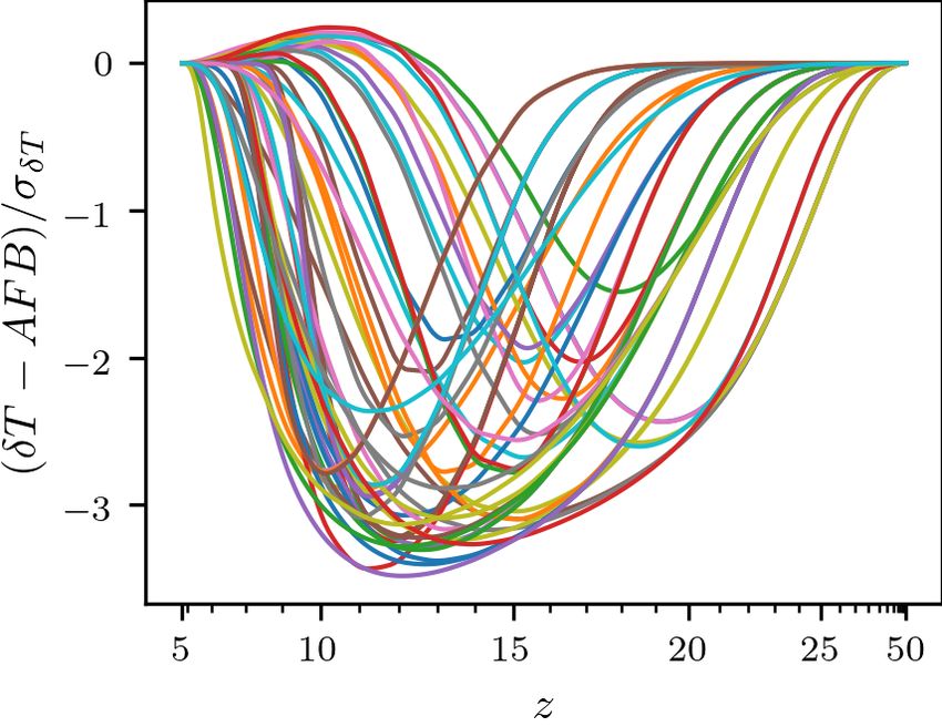
4 H. T. J. Bevins et al.
of in greater detail (Reis et al. 2021). However, the 21cmGEM data
is sufficient to demonstrate the abilities of globalemu.
 • : The power defining the slope of the X-ray SED with a range
given by 1 − 1.5. The Global 21-cm signal is expected to have a
very weak dependence on with the largest effect happening at low
redshifts.
 • min : The low energy cut off of the X-ray SED has a range of
0.1 − 3 keV. Low values of min correspond to a soft X-ray SED,
efficient X-ray heating and a weak absorption feature in the 21-cm
signal.
 • mfp : The mean free path of ionizing photons, with a range
10 − 50 Mpc. mfp is expected to have a very weak effect and only at
low redshifts (see e.g. Monsalve et al. 2019). A low mfp corresponds
to a slower ionization of the neutral hydrogen gas.
 • : The redshift of the 21-cm brightness temperature is a measure
of time and provides details about when each feature of the signal Figure 2. A subsample of 50 Global 21-cm signals from the 21cmGEM train-
occurred. For example the brightness temperature is expected to ing set used here to demonstrate the efficiency of globalemu. The signals
reach 0 mK, corresponding to the end of the EoR, at low redshifts show the expected variety of structure with deep and shallow absorption
or more recent times. It is interchangeable with frequency given that troughs caused by Lyman- coupling and terminated by X-ray heating. We
the rest frequency, , of the 21-cm line is 1420 MHz also see emission against the CMB background at low redshifts in some of
 the models where there has been sufficient heating. Also shown in black is the
 
 +1= . (1) Astrophysics Free Baseline (AFB) (section 4.1) which we model and remove
 from the training signals before we pass them through the neural network.
 To ensure that we make a fair comparison of our results with Subtraction of the AFB prevents our network from attempting to learn a
those found when using 21cmGEM we make the same physically steadily decreasing temperature at high redshifts prior to star formation.
motivated cuts to the test data as are detailed in section 2.4 of Cohen
et al. (2020). This equates to limits on the ionizing efficiency of
 is expected to be (and shown to be, section 6) simpler. We note
sources, < max = 40, 000 ∗ and on the neutral fraction history at
 that for & 30 the neutral fraction is expected to always be 1 and
 = 5.9, ( = 5.9) < 0.16. Respectively the limits are motivated
 so we only emulate the neutral fraction over the range = 5 − 30.
by stellar models (Bromm et al. 2001) and quasar absorption troughs
 The models have not been released publicly but the parameter ranges
(McGreer et al. 2014). We also note that some of the parameters in
 are the same for this data set as detailed above. A subsample of the
the testing data have different ranges and the ranges are as follows;
 training models is shown in Fig. 3.
 ∗ : 0.0001 − 0.5, : 4.2 − 76.5 km/s, : 0 − 10, : 0.055 − 0.1, :
 We note that a non-uniform coverage of the parameter space in
1 − 1.5, min : 0.1 − 3 keV and mfp : 10 − 50 Mpc. In total the final
 the training data set, as with the 21cmGEM data, may introduce
testing data set is comprised of 1703 models.
 bias in the neural network. The network will tend to learn regions
 globalemu includes a simple to use python graphical user in-
 of the astrophysical parameter space where the sampling is heavier
terface (GUI)2 in which the variation of the signal with each of the
 better than others. For the purposes of illustrating the accuracy of the
astrophysical parameters listed above can be explored in more detail.
 emulation in this paper this is not an issue. However, it can become
We note that the GUI is a feature made possible by the speed of emu-
 an issue when using an emulator to physically model a signal in a
lation when using globalemu (see section 6). There is an equivalent
 data set where parameter estimation may be biased towards a false
GUI for the neutral fraction history emulation.
 set of parameters. Training a network on a more uniform data set can
 As previously stated, globalemu is not limited to emulating sig-
 alleviate this issue.
nals modelled with the above astrophysical parameters. It is flexible
enough that more complicated astrophysical relationships can also
be emulated. For example one explanation for the unexpected depth
of the EDGES absorption trough is the presence of a higher than ex- 4 DATA PRE-PROCESSING
pected radio background which can be characterised with a quantity The details in the following discussion outline the pre-processing for
 radio determining the normalisation of the radio emissivity (assum- the network predicting the Global 21-cm signal. In section 4.4 we
ing the source of the excess radio background is stellar, Reis et al. briefly discuss the pre-processing for the neutral fraction networks
2020). globalemu is in principle capable of being trained on models which is a largely similar process. The pre-processing is summarised
that consider radio in addition to the above 7 astrophysical parameters as a flow chart in Fig. 4.
and redshift as inputs since it assumes nothing about the astrophysi-
cal parameters themselves. Equally globalemu could be trained on
less complex models. 4.1 Astrophysics Free Baseline Subtraction
 For the neutral fraction, , we use a set of models produced as a
by-product of the detailed 21cmGEM Global signal simulations. The In the region where the structure of the Global 21-cm signal is
data set is smaller with 10,047 training models and 791 test models expected to be dominated by collisional coupling it is independent
however the relationship between the astrophysical parameters and on the 7 astrophysical parameters used here as inputs to the emulator.
 This means that, in the corresponding redshift range, each of the
 signals in our training and testing data sets have the same brightness
2 After installation via pip or from source the GUI can be called from the temperatures. To prevent our network unnecessarily learning a non-
terminal using the command globalemu. See the documentation at https: trivial structure in this region we can treat it as an Astrophysics Free
//globalemu.readthedocs.io/ for more details. Baseline (AFB), model and remove it from the signals before they

MNRAS 000, 1–11 (2021)

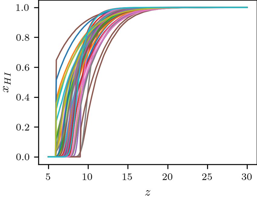
globalemu: Emulating the Global 21-cm signal 5

 Training Data
 (Section 3)

 Astrophysics Free
 Baseline
 (Section 4.1)

 Resampling
 (Section 4.2)
Figure 3. A subsample of 50 neutral fraction histories from the training set
used in this paper. At high redshift the hydrogen in the universe is predom-
inantly neutral and consequently = 1. As the gas is ionised by UV
emission from the first stars that form the neutral fraction decreases until
 Output Input
 = 0 at the end of the EoR.
 Normalisation Normalisation
 (Section 4.3) (Section 4.3)
are passed to the network for training. By doing this our network will
learn a simpler relationship at high redshift between the parameters
and ( ) than the existing steadily decreasing trend (see Fig. 2).
 In appendix A we give an approximate calculation of the AFB Neural Network
for the simulated signals that comprise the training data sets. The Training
calculation is approximate because it follows the mean evolution of (Section 5)
the signal and in contrast the simulations are produced over large
scale cosmological volumes evolved over cosmological time then Figure 4. The pre-processing applied to the training data in globalemu.
averaged. We therefore normalise our result to the temperature of the Each box is outlined in more detail in the corresponding sections. The red
signals in the training set at = 50 and find that this is sufficient to path is the pre-processing steps used for the Global 21-cm Signals, the blue
represent the astrophysics free component of the models. path for the neutral fraction histories and the gold path are steps that occur
 when training both neural networks.
 As stated, the AFB is then subtracted from the models before
training the network and added back in after making predictions.
 21cmGEM uses five extra parameters in addition to the seven subtracting the AFB, across the training data set
astrophysical parameters used here. Three of these additional pa-
rameters rely on the fraction of mass contained in halos above the Δ( ( )) = max ( ) − min ( ), (2)
minimum cooling threshold, coll ( ), and help the network learn the and we treat this as a probability distribution
signal structure at high redshift where collisional coupling (cosmol-
ogy) dominates. Here we do not consider these parameters as we are Δ( ( ))
 (Δ( ( ))) = Í . (3)
instead removing the AFB. The final two parameters, for reference, Δ( ( ))
are the fractions of X-ray energy above 1 keV and 2 keV. These pa- Where the variation in the signal at a given redshift across the
rameters are added to further characterise the X-ray SED but we find training data set is large the probability distribution is also large (see
with globalemu that we do not need to consider them to achieve Fig. 5). We then calculate the corresponding cumulative distribution
accurate results. function (CDF) and use inverse transform sampling to produce a
 new redshift distribution with a high sampling rate in regions of high
 variation. For each signal we can then perform an interpolation to
4.2 Resampling of signals get the corresponding values.
The turning points, and gradients between them, of the Global 21-cm
signal encode all of the information about the efficiency of Lyman- 
 4.3 Output and Input Normalisation
coupling, X-ray heating and reionization. They are therefore highly
dependent on the relevant astrophysical parameters and in the region Neural networks typically perform better when the outputs and inputs
where the features typically occur variation in the signals is signif- are of order unity and uniformly distributed. Hence it is typical to
icant. The original signal models are sampled uniformly in redshift manipulate the data sets via logarithms, normalisation and/or stan-
and there is not particular physical motivation for this. However, to dardisation to improve performance.
improve the quality of modelling we resample the signals at a higher After subtracting the AFB and resampling our signals we also
rate across the redshift ranges that typically correspond to the lo- proceed to divide the signals by the standard deviation across the
cations of the turning points and at a lower rate where the signal training data set. This type of scaling was motivated by the typically
structure deviates less from the ‘average’ signal (e.g. above ≈ 30 used standardisation technique however we wanted to ensure that
where the signal is free of astrophysics). when scaling our signals a value of = 0 remained as 0 because it
 To do this we look at the variation in the signal amplitudes, after holds physical meaning (an equivalence between the spin temperature

 MNRAS 000, 1–11 (2021)

6 H. T. J. Bevins et al.

 Figure 6. The equivalent signals from Fig. 2 after pre-processing. Subtraction
 of the AFB and the subsequent resampling mean that the important informa-
 tion encoding the dependence on the astrophysical parameters is retained and
 appropriately emphasised in the training data. Here we have plotted the re-
 sampled redshift data points as being uniformly distributed since this is how
 the network is set up to interpret the input. The following division by the
 standard deviation across the training data set scales the signals to order unity
 without changing the physically significant value of ( ) = 0 where the
 spin temperature of the neutral hydrogen is equivalent to the radio background
 temperature. Minor ticks are at intervals of one on the x-axis.

 For , ∗ and the distributions are uniform in log-space and
 so we perform the Min-Max normalisation on the logarithm of these
 variables and use these as our inputs.

Figure 5. Top panel: The probability distribution calculated from the dif-
ference between the maximum and minimum signal temperatures in the 4.4 Pre-processing
21cmGEM training data set using equation (2) and equation (3). Bottom
 As discussed we provide provision in globalemu to emulate the
panel: The cumulative distribution function (CDF) corresponding to the
 neutral fraction of hydrogen as a function of redshift. For this network
probability distribution in the top panel. We use this CDF to resample the
training Global 21-cm signals in order to capture the variation at low redshifts the pre-processing just involves resampling of the signals since:
across the distribution and allow the emulator to better learn this behaviour.
 • The equivalent AFB for the neutral fraction has a value of 1
 at all redshifts and to subtract this from our training data set would
and radio background, = ). The signals shown in Fig. 2, as seen invert our signals providing no benefit to training.
by the neural network, after pre-processing are shown in Fig. 6. • The neutral fraction has a value between 0 and 1 by definition
 For the input redshift distribution we transform our resampled and so we do not need to normalise the output of the network to be
redshifts back onto a uniform distribution between 0 and 1, before of order unity.
they are input into the network, using the CDF detailed in the previous
 The benefits of performing resampling for the neutral fraction
section. It is the combination of resampling and uniform redshift input
 histories are the same as for the Global signal network. It allows the
that ensures the neural network ‘sees’ ‘stretched’ signals as in Fig. 6.
 network to learn the variation in the training models and interpolation
This technique allows the neural network to interpolate the signal
 across redshift with a higher degree of accuracy. We perform the
at redshifts it hasn’t been trained on to a higher degree of accuracy
 resampling with the equivalent of equation (2) and equation (3).
where the signals vary greatly than if we had used uniform sampling.
 Fig. 7 shows the same set of neutral fraction histories as in Fig. 3
 For the other input astrophysical parameters we use a Min-Max after pre-processing.
normalisation scaling each feature between 0 and 1. For example,
considering the distribution of the CMB optical depth, in our
training data as a vector we normalise it such that
 − min
 ˜ = . (4)
 max − min 5 NEURAL NETWORK STRUCTURE
The decision to use this type of normalisation was arrived at after As stated, the goal with globalemu is to maintain a simple network
testing standardisation, Min-Max normalisation and division by the that is highly accurate without having to use dropout, regularisation,
max values for the input parameters while maintaining the physically batch normalisation etc. However, in the design of any neural network
motivated pre-processing for the signal temperatures detailed in the the optimizer, the architecture, loss function, activation function and
above sub-sections. learning rate are core considerations.

MNRAS 000, 1–11 (2021)

globalemu: Emulating the Global 21-cm signal 7

Figure 7. The equivalent neutral fraction histories from Fig. 3 after pre-
processing. For the neutral fraction histories, since the signals are already of
order unity and subtraction of the equivalent AFB would not be beneficial,
the pre-processing just involves resampling of the signals around regions of
high variation. As with Fig. 6 the minor ticks are at intervals of one on the
x-axis.

5.1 Architecture
Dropout (Srivastava et al. 2014) and the commonly used L1 and L2
regularisation are typically employed to prevent overfitting where the Figure 8. The mean and 95 percentile (see section 6.2) for a set of
network learns the training data to such a high degree of accuracy different network architectures trained for 12h (approximately 250 epochs)
that it is unable to generalise. Overfitting is generally a result of on a HPC with the 21cmGEM Global signal training data and assessed with
using a neural network that is too big and has an excessive number the corresponding test data. The architectures have between 1 and 4 layers of
 varying sizes between 4 and 64 nodes. They are ordered based on the number
of layers and nodes. On the other hand a network that is too small
 of weights in the network (equivalent to the number of connections) as this is
often produces poor quality predictions and consequently the aim is to
 a useful measure of network size and an indication of predictive power. The
produce a ‘reasonably’ sized network. The scope of what constitutes a graph is used to determine a ‘reasonable’ architecture considering the practical
reasonably sized network is dependent on the number of input/output target accuracy of on average 10% the expected noise of a Global 21-cm
nodes, the variation in the training data and the complexity of the experiment (here illustrated by the black dashed line at 2.5 mK). Throughout
relationship between the inputs and outputs. the rest of the paper we use a network with 3 layers each consisting of 16
 By using the novel approach of having redshift as an input to the nodes which is the first to produce a mean value within our target accuracy.
network both our Global signal and neutral fraction emulators have, in Our choice is highlighted with a dotted vertical line.
the case of the 21cmGEM data, eight input nodes and one output node
meaning that our network can remain small in size. Additionally, we
have made a significant effort to simplify the problem with physically Fig. 8 illustrates the processes used to determine our architec-
motivated pre-processing which also helps to reduce what constitutes ture for the Global network. We consider a set of different net-
as ‘reasonable’ size for our networks. work sizes with one to four layers and 4, 8, 16, 32 or 64 nodes
 globalemu is set up in such a way that the number of layers and in each layer. For each of the tested networks we run a ‘full’, 12
layer sizes can be adjusted by the user. As a result we do not provide hours on a HPC equating to approximately 250 epochs using the full
a prescription of what constitutes a ‘reasonable’ size as this may 21cmGEM training data, training of globalemu. We then assess the
not be pragmatic. We note, however, that a significant effort can be accuracy of the trained models using the ≈ 1, 700 testing models
undertaken to determine the optimum ‘reasonable’ architecture that in the 21cmGEM dataset. We compare the mean and 95 percentile
maximises accuracy and that this can also be impractical. Instead we (see section 6.2) for each architecture. We find that a network
suggest that as a minimum requirement a ‘reasonable’ architecture of size [16, 16, 16] is the first to meet our target accuracy of on
for a trained globalemu model should meet the following criteria: average 10% the expected noise in a Global 21-cm experiment.
 While we may be able to achieve a better accuracy with a larger
 • The network should not over fit the training data otherwise the network this pragmatic approach leads to a sufficiently accurate net-
predictive power will be lost. work for physical signal modelling in the data analysis pipeline of
 • The network should have an average accuracy . 10% the noise a Global experiment like REACH. We also note that a smaller net-
of a typical Global 21-cm experiment (see section 6.2 for a further work can be evaluated faster than a larger architecture and that this is
discussion). important when we are making multiple evaluations inside a nested
 sampling loop.
 Based on the above criteria, the size of our input and output layers
and a minimal exploration starting from a small network, trained with
the pre-processed signals, and increasing the size until our accuracy
 5.2 Loss Function and Learning rate
criteria was met without overfitting we use a network with 3 hidden
layers all of size 16 for both the Global signal and neutral fraction globalemu uses the Mean Squared Error, typical for a regression
emulation in this paper. network, as the loss function. In the case of the Global signal network

 MNRAS 000, 1–11 (2021)

8 H. T. J. Bevins et al.
is given by emulating the 1,703 test models and taking an average time per sig-
 
 nal. The tests are performed with matlab and python respectively
 1 ∑︁ on the same computer with the following processors: Intel® Core™
 = ( sim,i ( ) − pred,i ( )) 2 (5)
 
 =0
 i3-10110U CPU @ 2.10GHz × 4. For 21cmGEM we make a vec-
 torised call to the emulator as this results in a quicker performance
where is a batch size equivalent to the number of redshift data then repeated single calls. We use a for loop to repeatedly call glob-
points in each signal. sim ( ) is the simulated signal temperature alemu which currently doesn’t support such vectorised calls as they
at a given redshift and pred ( ) is the emulated equivalent. glob- are not needed for physical signal modelling in a nested sampling
alemu trains the neural networks in batches primarily to prevent loop.
memory related issues since the training data can be large (≈ 27, 000 For globalemu we record a total time of 2.29 s and a corre-
models times 451 redshift points ≈ 12 million data points for the sponding average time per signal of 1.3 ± 0.01 mK. In compar-
21cmGEM data). We find that a reasonable batch size is equal to the ison when emulating the same signals in a vectorised call with
number of redshift data points in each model. 21cmGEM we record a total time of 227.18 s and an average
 For the 21cmGEM data and the globalemu framework we deter- time per signal of 133 ms. We therefore achieve a factor of 102
mine an effective learning rate to be 0.001. As with the architecture improvement in emulation time with globalemu. We note that
the learning rate can be adjusted by the user of globalemu to meet when using the pymatbridge (https://github.com/arokem/
the requirements of the data that they are training on. python-matlab-bridge) python wrapper for matlab the aver-
 age time take to run a single prediction with 21cmGEM using a
 vectorised call is comparable to a direct call in matlab.
5.3 Optimizer
The neural network optimizer is used to change the networks hyper-
parameters to minimise the loss function. There is a number of dif- 6.2 Measuring Accuracy
ferent optimizers available (Ruder 2016) and the choice can be de- In this section we primarily consider the accuracy of the Global
pendent on the complexity of the problem and loss surface. A more signal emulator because the neutral fraction network has a similar
robust optimizer is less likely to fall into and get stuck in local min- design. We note, as previously stated, that the relationship between
ima when training the network resulting in more accurate emulation. the neutral fraction and the astrophysical parameters is expected to
Therefore the choice of optimizer is important in designing an effec- be simpler and therefore easier to learn.
tive emulator. However, since globalemu is designed to minimise To assess the accuracy of globalemu when emulating a Global
the complexity of the relationship between the inputs and outputs and 21-cm signal simulation we use a combination of two metrics; the
a MSE loss surface is relatively smooth3 our choice is less consequen- root mean squared error ( ) and the normalised given
tial. We use, therefore, the commonly applied ADAM (Kingma & in Cohen et al. (2020) as
Ba 2014) optimizer which is a momentum based modified stochastic
gradient descent algorithm. 
 =
 Ÿ , (6)
 | sim ( )|
 where
5.4 Activation Functions v
 u
 t 
For both the Global signal and neutral fraction history network, we 1 ∑︁
 = ( sim,i ( ) − pred,i ( )) 2 . (7)
use a tanh activation function in the hidden layers which can range 
 =0
between (-1, 1). However, for our final layer in the Global signal net-
 For the neutral fraction network Ÿ and (with sim ( )
work we use a linear activation since the pre-processed temperature
can be positive or negative and range between approximately −4 and and the equivalent for the emulation in place of temperature) are
 ( )| = 1. We assess the accuracy in the uniform
 equal since | sim
0.5. Similar consideration is given to the output layer in the neutral
fraction network where we use a ReLU (Rectified Linear Unit) ac- redshift space and consequently our assessment is independent of the
tivation which ensures that the output is always positive. Again the loss function used for training.
activation functions can be changed by the user of globalemu to is a dimensionless quantity used by 21cmGEM and by
 Ÿ
meet the requirements of their data. We note that the above output assessing the quality of our network with this metric we can make
layer activations are designed to prevent unphysical outputs and that direct comparisons between the two emulators. We also want our
this is a crucial consideration for any user. emulator to have an accuracy significantly lower than the expected
 noise floor of Global 21-cm experiments. This is required if the
 emulator is to be used to confidently model the Global 21-cm signal
 and draw conclusions about the astrophysics during the CD and EoR.
6 RESULTS
 To assess this accuracy requirement we can use the dimensionful
6.1 Emulation Time metric.
 As highlighted in the previous section, we suggest an average ac-
In Cohen et al. (2020) the reported average time taken per signal with
 curacy of . 10% the expected noise of a Global 21-cm experiment
21cmGEM is 160 ms when emulating a set of signals in a vectorised
 such as REACH, equivalent to an . 2.5 mK, to be a suf-
call. Here we compare the speed of 21cmGEM and globalemu by
 ficient limit. Since the accuracy of emulation is a function of the
 bandwidth, we report the accuracy across the entire range of the
3 This can be assessed with a plot of the loss vs epoch number during training. simulations = 5 − 50 ( = 5 − 30 for the neutral fraction network)
We find that for the results presented in section 6 the surface is smooth up and across the expected REACH Phase I bandwidth of = 7 − 28
until the loss has plateaued and training is complete at which point we see (REACH Collaboration 2021 (in prep.)). The target is demonstra-
noise like behaviour. tively achievable (see following section). It is also a practical target,

MNRAS 000, 1–11 (2021)

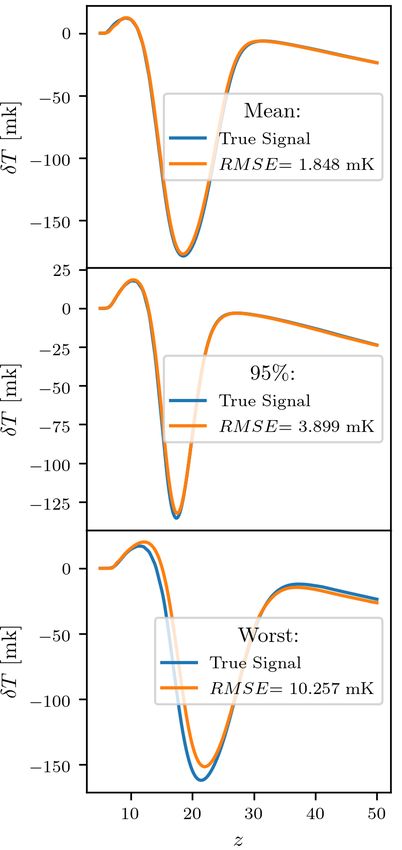
globalemu: Emulating the Global 21-cm signal 9
if we want to use globalemu for physical signal modelling, given
that the noise in a 21-cm experiment has a fundamental effect on our
confidence in any astrophysical parameter values inferred from the
data and that this will likely be larger than the uncertainty introduced
from globalemu.

6.3 Global 21-cm Signal
Fig. 9 shows that the mean value across the redshift range
 = 5 − 50 is 1.85 mK and that the maximum value is 10.26 mK.
Further, Tab. 1 shows that performing the same calculation of the
 inside the REACH band, = 7 − 28 gives a mean value of
2.52 mK which is very close to the desired 2.5 mK limit. We also
report in the table the value for which 95% of the models
have a value smaller than or equal to. In the REACH band this
equates to 5.37 mK. For all of the reported results the 95 percentile
is significantly lower than the maximum values (a factor of 3 for
the Global signal and a factor of approximately 1.5 to 2 depending
on bandwidth for the neutral fraction histories). This means that out
of a set of 1, 703 Global signals only 85 have values above
3.90 mK across the band = 5 − 50 for example. We note that the
values reported, averages across redshift ranges, in the REACH band
are generally higher than across the whole redshift range because
the REACH band excludes redshifts & 30 where the emulation is
expected to be very precise.
 Appendix B shows the explored parameter space for the Global
21-cm signal in the 21cmGEM test data set and the corresponding
error when emulating the signals with globalemu.
 Finally, in Tab. 1 we also report the Ÿ values in both the
REACH band and across the whole redshift range. Cohen et al.
(2020) report similar results for 21cmGEM and particularly we note
that, when training and testing on the same data sets, we recover a
mean Ÿ of 1.12% compared to 1.59% when using 21cmGEM.
Similarly we report a maximum value of 6.32% in comparison to
the value of 10.55% reported by Cohen et al. for 21cmGEM. This
further demonstrates that globalemu can achieve a high degree of
accuracy in its emulation.
 Figure 9. The figure shows the mean, 95 percentile and the worst emulations,
 based on the , for the Global 21-cm signal across the entire test set
6.4 Neutral Fraction of 1,703 models. Full details of the accuracy of the emulation can be found
 in Tab. 1 and a discussion can be found in the text.
For the neutral fraction history network we show similar results.
Fig. 10 demonstrates the quality of the emulation with the mean, 95
percentile and the worst results when emulating the neutral fraction resample both the Global signals and neutral fractions so that the
and these values are detailed in Tab. 1. The results generally are of regions which vary significantly across the training data sets can be
higher quality than that for the Global signal and, noting that the pre- better characterised by the networks.
processing for the two networks is near identical and the networks The above framework allows the complex relationships between
themselves are of the same size, this supports the understanding that the astrophysical parameters and the Global signal or neutral fraction
the relationship between the inputs and outputs is simpler here. In the history as functions of redshift to be effectively learnt with small
band = 5 − 50 only 39 of 791 test models have Ÿ ≥ 0.47%. neural networks. Each Global signal of 451 redshift data points can
 be emulated in on average 1.3 ms. We note that this is a factor
 of approximately 102 improvement on the 133 ms we record with
 matlab when predicting the same signals on the same computer with
7 CONCLUSIONS
 21cmGEM.
globalemu uses a novel approach to emulate, with neural networks, We demonstrate the effectiveness of globalemu by using the
the Global 21-cm signal and the evolution of the neutral fraction 21cmGEM training and testing data. This allows for a direct compar-
during the CD and EoR by considering redshift as an input to the ison between our results and the results of 21cmGEM. We find that
neural networks alongside the astrophysical parameters. In tandem globalemu can emulate to a higher degree of accuracy the Global
with this reparameterisation of the problem we use a predominantly 21-cm signal than 21cmGEM with a maximum normalised 
physically motivated pre-processing for both the Global signal and of 6.32% in comparison to 10.55% over the range = 5 − 50. We
neutral fraction. We subtract from the Global signals an astrophysics also demonstrate that globalemu can emulate a Global 21-cm signal
free baseline which obviates the need for the network learning a non- to, on average, less than 10% the expected noise of a Global 21-cm
trivial but well-understood relationship at high redshift. We then experiment like REACH.

 MNRAS 000, 1–11 (2021)

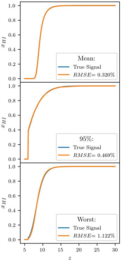
10 H. T. J. Bevins et al.
 Global Signal Neutral Fraction

 = 5 − 50 = 7 − 28 = 5 − 30 = 7 − 28

 Minimum 0.30 mK 0.31 mK 0.09% 0.08%
 Mean 1.85 mK 2.52 mK 0.29% 0.26%
 
 95 ℎ percentile 3.90 mK 5.37 mK 0.47% 0.44%
 Maximum 10.26 mK 15.10 mK 1.12% 0.65%

 Minimum 0.21% 0.26% – –
 Mean 1.12% 1.53% – –
 
 Ÿ 
 95 ℎ percentile 2.41% 3.22% – –
 Maximum 6.32% 9.31% – –
Table 1. Detailed results of the emulation using globalemu and the 21cmGEM training and test data for both the Global signal and the neutral fraction history.
We find that globalemu achieves the desired accuracy of on average ≈ 10% the expected noise of a typical Global 21-cm experiment (equating to ≈ 2.5 mK in
the REACH band of = 7 − 28). Of note are the recorded 95% percentiles, the for which 95% of the models have values smaller than or equal to, which
are significantly lower than the maximum values. A discussion comparing the results of 21cmGEM and globalemu, in terms of Ÿ , can be found
in the text. Briefly we find that our Global signal emulator has a maximum 
 Ÿ approximately half that achieved with 21cmGEM. For the neutral fraction
 = Ÿ and so we only report one set of results. We find a higher degree of accuracy here with an identical network and similar pre-processing
indicating a simpler relationship.

 Finally, globalemu is a flexible python package that can be easily Cohen A., Fialkov A., Barkana R., Monsalve R. A., 2020, MNRAS, 495,
retrained on updated models with new astrophysical dependencies. 4845
For example additional astrophysical phenomena such as Lyman- Cohen A., Fialkov A., Barkana R., Monsalve R. A., 2021, 21cmGEM Training
heating (Reis et al. 2021) or additional radio background produced and Testing Data Sets, doi:10.5281/zenodo.4541500
by galaxies (or an indeterminate synchrotron-like source) (Fialkov de Lera Acedo E., 2019, in 2019 International Conference on Elec-
 tromagnetics in Advanced Applications (ICEAA). pp 0626–0629,
& Barkana 2019; Reis et al. 2020) can be incorporated and easily
 doi:10.1109/ICEAA.2019.8879199
trained upon. While the results achieved with the 21cmGEM data are
 Fialkov A., Barkana R., 2014, Monthly Notices of the Royal Astronomical
impressive, the novelty of globalemu is in its flexibility, incorpora- Society, 445, 213
tion of redshift as an input and physically motivated pre-processing. Fialkov A., Barkana R., 2019, Monthly Notices of the Royal Astronomical
Particularly the final two points allow for an accurate mapping from Society, 486, 1763
parameters to temperature with a single neural network reducing the Field G. B., 1959, ApJ, 129, 536
points of failure and need for excessive fine-tuning. Furlanetto S. R., Oh S. P., Briggs F. H., 2006, Phys. Rep., 433, 181
 Handley W. J., Hobson M. P., Lasenby A. N., 2015a, MNRAS, 450, L61
 Handley W. J., Hobson M. P., Lasenby A. N., 2015b, MNRAS, 453, 4384
 Hills R., Kulkarni G., Meerburg P. D., Puchwein E., 2018, Nature, 564, E32
ACKNOWLEDGEMENTS
 Ioffe S., Szegedy C., 2015, arXiv e-prints, p. arXiv:1502.03167
HB acknowledges the support of the Science and Technology Facili- Javid K., Handley W., Hobson M., Lasenby A., 2020, arXiv e-prints, p.
ties Council (STFC) through grant number ST/T505997/1. WH and arXiv:2004.12211
AF were supported by Royal Society University Research Fellow- Kingma D. P., Ba J., 2014, arXiv e-prints, p. arXiv:1412.6980
 Liu A., Shaw J. R., 2020, PASP, 132, 062001
ships. EA was supported by the STFC through the Square Kilometer
 Madau P., Meiksin A., Rees M. J., 1997, ApJ, 475, 429
Array grant G100521.
 McGreer I. D., Mesinger A., D’Odorico V., 2014, Monthly Notices of the
 Royal Astronomical Society, 447, 499
 Mesinger A., 2019, The Cosmic 21-cm Revolution; Charting the first billion
DATA AVAILABILITY years of our universe, doi:10.1088/2514-3433/ab4a73.
 Mesinger A., Furlanetto S., Cen R., 2011, 21cmFAST: A Fast, Semi-
The Global 21-cm signals used in this paper are publicly available at Numerical Simulation of the High-Redshift 21-cm Signal (ascl:1102.023)
https://doi.org/10.5281/zenodo.4541500 and provided by Mittal S., Kulkarni G., 2020, MNRAS,
Cohen et al. (2021). Monsalve R. A., Fialkov A., Bowman J. D., Rogers A. E. E., Mozdzen T. J.,
 Cohen A., Barkana R., Mahesh N., 2019, ApJ, 875, 67
 Pearson K., 1901, The London, Edinburgh, and Dublin Philosophical Maga-
 zine and Journal of Science, 2, 559
REFERENCES Philip L., et al., 2019, Journal of Astronomical Instrumentation, 8, 1950004
Anstey D., de Lera Acedo E., Handley W., 2020, arXiv e-prints, p. Planck Collaboration VI 2020, A&A, 641, A6
 arXiv:2010.09644 Price D. C., et al., 2018, MNRAS, 478, 4193
Barkana R., 2016, Phys. Rep., 645, 1 Pritchard J. R., Loeb A., 2012, Reports on Progress in Physics, 75, 086901
Bevins H. T. J., Handley W. J., Fialkov A., Acedo E. d. L., Greenhill L. J., Reis I., Fialkov A., Barkana R., 2020, MNRAS, 499, 5993
 Price D. C., 2021, MNRAS Reis I., Fialkov A., Barkana R., 2021, arXiv e-prints, p. arXiv:2101.01777
Bowman J. D., Rogers A. E., Monsalve R. A., Mozdzen T. J., Mahesh N., Ruder S., 2016, arXiv e-prints, p. arXiv:1609.04747
 2018, Nature, 555, 67 Sims P. H., Pober J. C., 2020, MNRAS, 492, 22
Bromm V., Kudritzki R. P., Loeb A., 2001, ApJ, 552, 464 Singh S., Subrahmanyan R., 2019, ApJ, 880, 26
Chatterjee A., Choudhury T. R., Mitra S., 2021, arXiv e-prints, p. Singh S., Subrahmanyan R., Udaya Shankar N., Sathyanarayana Rao M.,
 arXiv:2101.11088 Girish B. S., Raghunathan A., Somashekar R., Srivani K. S., 2018, Ex-
Chuzhoy L., Shapiro P. R., 2007, ApJ, 655, 843 perimental Astronomy, 45, 269
Cohen A., Fialkov A., Barkana R., Lotem M., 2017, MNRAS, 472, 1915 Srivastava N., Hinton G., Krizhevsky A., Sutskever I., Salakhutdinov R.,

MNRAS 000, 1–11 (2021)

globalemu: Emulating the Global 21-cm signal 11
 temperature, , via the collisions and that temperature cools adia-
 batically at a faster rate than the background radiation, . The spin
 temperature, , which encodes the number of hydrogen atoms in
 the two hyperfine levels of the ground state (Furlanetto et al. 2006)
 during this period is given by
 1 1/ + / 
 = (A1)
 1 + 
 where is the collisional coupling coefficient. For our approxima-
 tion of the AFB calculated here we use a reference value for the gas
 temperature of ,ref = 33.7340 K at ref = 40 from the simulations
 used to produce the training and test data sets. We then scale ,ref
 adiabatically using
 (1 + ) 2
 = ,ref (A2)
 (1 + ref ) 2
 to get as a function of redshift.
 The coupling is dominated by H-H collisions and so we only
 consider these in our simulation. The coupling coefficient for this
 interaction is given by Furlanetto et al. (2006)
 
 10 ∗
 = , (A3)
 10 
 where 10 is the rate coefficient for the spin deactivation of neutral
 hydrogen, ∗ is the energy defect and 10 is the spontaneous emission
 coefficient of the 21-cm transition. is the relative number density
 of neutral hydrogen given by as
 
 = 3.40368 × 1068 (1 − )Ω (1 + ) 3 (A4)
 
 where = 0.274 and is the Helium abundance by mass, is critical
 mass density of the universe in sol /cMpc3 , is the proton mass
 in sol and Ω the the baryon density parameter.
 From the above we can then calculate as
 − 
 = (1 − exp(− 0 )), (A5)
 1+ 
Figure 10. The figure shows the mean, 95 percentile and the worst emulations where 0 is the 21-cm optical depth of the diffuse IGM
for the neutral history across the entire test set of 791 models. The level of
 3ℎ 3 10 
accuracy here is higher than that for the Global signal, despite using a similar 0 = , (A6)
pre-processing and identical network, demonstrating that the relationship 32 02 ( )
between the astrophysical parameters, redshift and the network output is
simpler here. where 0 is the rest frequency of the 21-cm emission and ( ) is
 the Hubble rate. In our calculation we use the same cosmological
 parameters that were used to generate the signals (see Cohen et al.
 2014, Journal of Machine Learning Research, 15, 1929 2020). Here the neutral fraction, has a value of 1 since there is
Venumadhav T., Dai L., Kaurov A., Zaldarriaga M., 2018, Phys. Rev. D, 98, no astrophysics involved in the AFB.
 103513
Villanueva-Domingo P., Mena O., Miralda-Escudé J., 2020, Physical Review
 D, 101, 083502 APPENDIX B: ERROR VS PARAMETER
Visbal E., Barkana R., Fialkov A., Tseliakhovich D., Hirata C. M., 2012,
 Nature, 487, 70 Fig. B1 shows the parameter space explored in the 21cmGEM test
Wouthuysen S. A., 1952, AJ, 57, 31 data set as a scatter plot. The data points are coloured based on
 the value calculated when comparing the corresponding true
 signal with the emulation, over the range = 5−50, from globalemu.
 Fig. B2 shows the equivalent graph with the colours determined
APPENDIX A: CALCULATING THE ASTROPHYSICS using the dimensionless Ÿ metric across the band = 5 − 50.
FREE BASELINE
To approximate the astrophysics free baseline (AFB) we need to This paper has been typeset from a TEX/LATEX file prepared by the author.
consider the physics defining the signal structure during the period
dominated by collision coupling. During this period neutral hydro-
gen atoms collide with other neutral hydrogen atoms, protons and
electrons. The spin temperature of hydrogen is coupled to the gas

 MNRAS 000, 1–11 (2021)

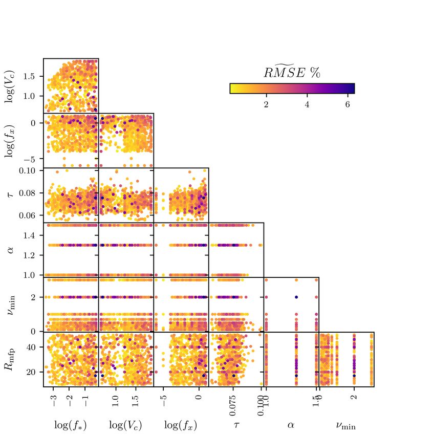
12 H. T. J. Bevins et al.

Figure B1. The parameter space explored by the 21cmGEM test data set. Each panel shows the 1, 703 models plotted as data points based on the corresponding
astrophysical parameter values. They are coloured according to the calculated when comparing the true signals to the emulation from globalemu across
the range = 5 − 50.

MNRAS 000, 1–11 (2021)