Hardware Acceleration of DNNs - Lecture 7: Visual Computing Systems Stanford CS348K, Spring 2021

Page created by Maurice Sutton
 
CONTINUE READING
Hardware Acceleration of DNNs - Lecture 7: Visual Computing Systems Stanford CS348K, Spring 2021
Lecture 7:

Hardware Acceleration
      of DNNs
    Visual Computing Systems
  Stanford CS348K, Spring 2021
Hardware Acceleration of DNNs - Lecture 7: Visual Computing Systems Stanford CS348K, Spring 2021
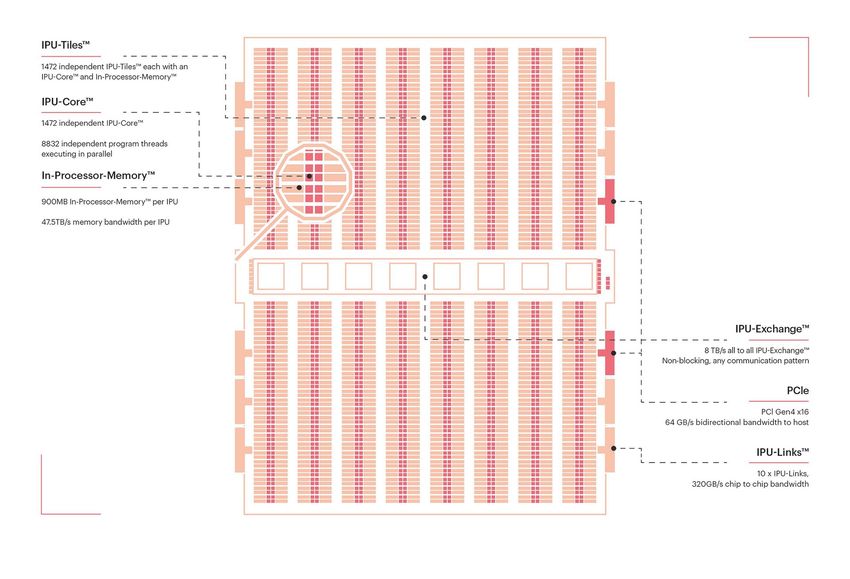
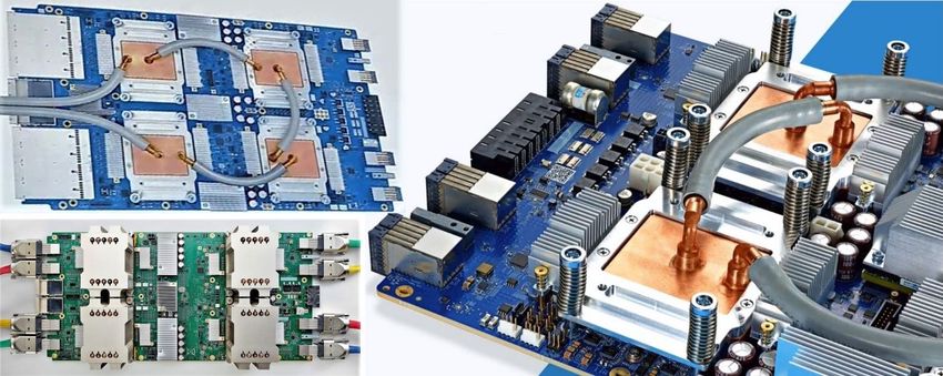
Hardware acceleration of DNN inference/training

                                                   Huawei Kirin NPU

      Google TPU3                            GraphCore IPU

                                                                      Apple Neural Engine

     Intel Deep Learning
    Inference Accelerator
                                           SambaNova
                                          Cardinal SN10

                                                                             Ampere GPU with
                                                                               Tensor Cores
            Cerebras Wafer Scale Engine
                                                                              Stanford CS348K, Spring 2021
Hardware Acceleration of DNNs - Lecture 7: Visual Computing Systems Stanford CS348K, Spring 2021
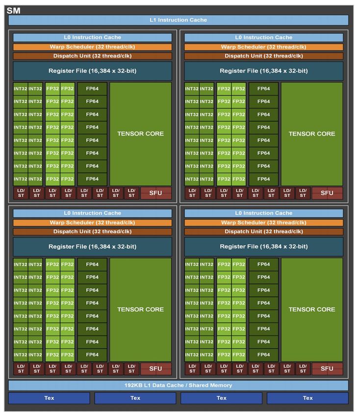
Investment in AI hardware

      NVIDIA Market Cap
         2014 - 2021

                            Stanford CS348K, Spring 2021
Hardware Acceleration of DNNs - Lecture 7: Visual Computing Systems Stanford CS348K, Spring 2021
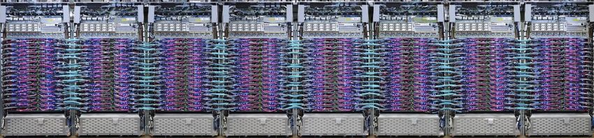
Two computer architecture reminders

                                Stanford CS348K, Spring 2021
Hardware Acceleration of DNNs - Lecture 7: Visual Computing Systems Stanford CS348K, Spring 2021
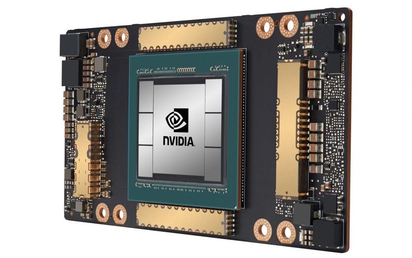
Compute specialization = energy efficiency
   ▪ Rules of thumb: compared to high-quality C code on CPU...

   ▪ Throughput-maximized processor architectures: e.g., GPU cores
          -   Approximately 10x improvement in perf / watt
          -   Assuming code maps well to wide data-parallel execution and is compute bound

   ▪ Fixed-function ASIC (“application-specific integrated circuit”)
          -   Can approach 100-1000x or greater improvement in perf/watt
          -   Assuming code is compute bound and
              and is not floating-point math

[Source: Chung et al. 2010 , Dally 08]                  [Figure credit Eric Chung]
                                                                                     Stanford CS348K, Spring 2021
Hardware Acceleration of DNNs - Lecture 7: Visual Computing Systems Stanford CS348K, Spring 2021
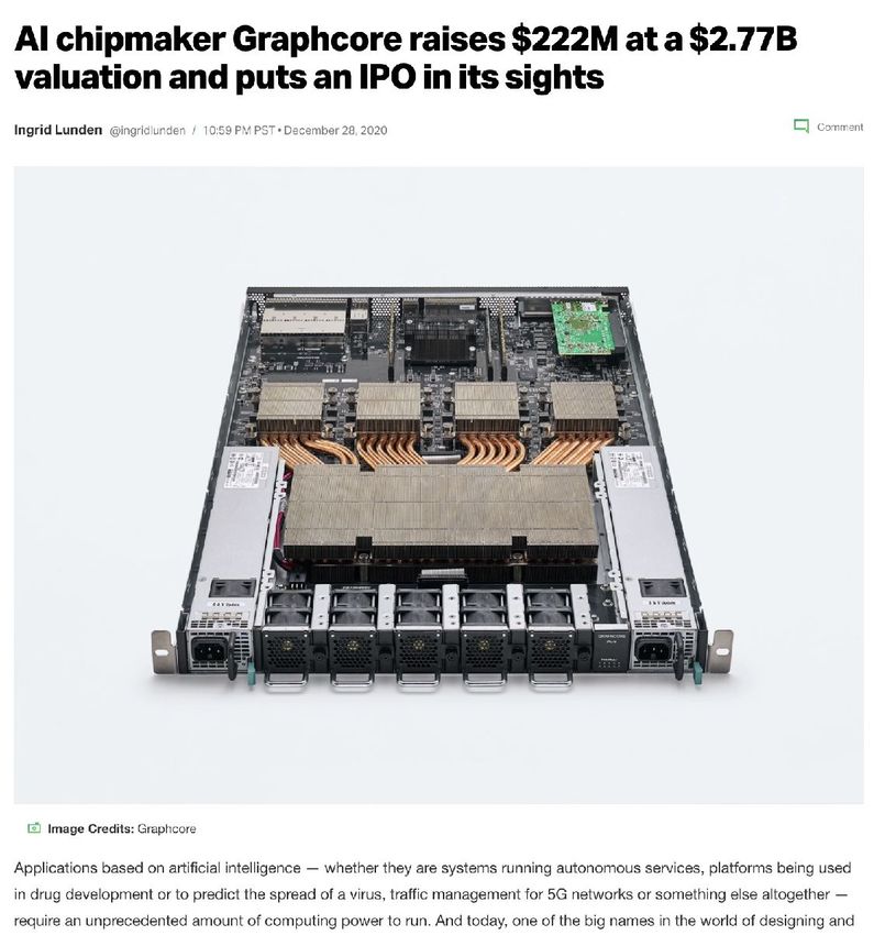
Data movement has high energy cost
   ▪ Rule of thumb in modern system design: always seek to reduce amount of
         data movement in a computer

   ▪ “Ballpark” numbers                                                                      [Sources: Bill Dally (NVIDIA), Tom Olson (ARM)]

          -   Integer op: ~ 1 pJ *
          -   Floating point op: ~20 pJ *
          -   Reading 64 bits from small local SRAM (1mm away on chip): ~ 26 pJ
          -   Reading 64 bits from low power mobile DRAM (LPDDR): ~1200 pJ

   ▪ Implications
          -   Reading 10 GB/sec from memory: ~1.6 watts
          -   Entire power budget for mobile GPU: ~1 watt
              (remember phone is also running CPU, display, radios, etc.)
          -   iPhone 6 battery: ~7 watt-hours (note: my Macbook Pro laptop: 99 watt-hour battery)
          -   Exploiting locality matters!!!

* Cost to just perform the logical operation, not counting overhead of instruction decode, load data from registers, etc.
                                                                                                                            Stanford CS348K, Spring 2021
Hardware Acceleration of DNNs - Lecture 7: Visual Computing Systems Stanford CS348K, Spring 2021
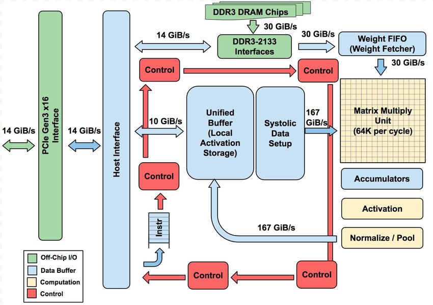
On-chip caches locate data near processing
                    Processors run efficiently when data is resident in caches
                            Caches reduce memory access latency *
                          Caches reduce the energy cost of data access

                         L1 cache
                          (32 KB)

  Core 1
                         L2 cache
                         (256 KB)

                                                             38 GB/sec           Memory
                    .                                                            DDR4 DRAM
                    .                    L3 cache
                    .                     (8 MB)                                 (Gigabytes)
                         L1 cache
                          (32 KB)

  Core N
                         L2 cache
                         (256 KB)

* Caches also provide high bandwidth data transfer to CPU                        Stanford CS348K, Spring 2021
Hardware Acceleration of DNNs - Lecture 7: Visual Computing Systems Stanford CS348K, Spring 2021
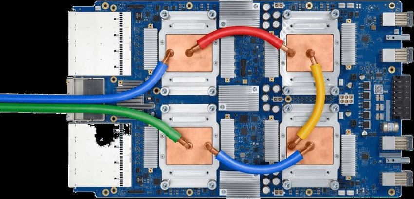
Memory stacking locates memory near chip
Example:
NVIDIA A100 GPU

Up to 80 GB HMB2 stacked memory
2 TB/sec memory bandwidth

Also note: A100 has 40 MB L2 cache
(increased from 6.1 MB on V100)

                                     Stanford CS348K, Spring 2021
Hardware Acceleration of DNNs - Lecture 7: Visual Computing Systems Stanford CS348K, Spring 2021
Improving hardware efficiency
     for DNN operations

                                Stanford CS348K, Spring 2021
Hardware Acceleration of DNNs - Lecture 7: Visual Computing Systems Stanford CS348K, Spring 2021
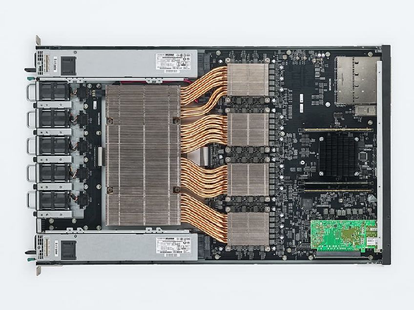
Amortize overhead of instruction stream
control using more complex instructions
▪ Fused multiply add (ax + b)
▪ 4-component dot product x = A dot B
▪ 4x4 matrix multiply
   -   AB + C for 4x4 matrices A, B, C

▪ Key principle: amortize cost of instruction stream processing
   across many operations of a single complex instruction

                                                            Stanford CS348K, Spring 2021
Efficiency estimates *
 ▪ Estimated overhead of programmability (instruction stream, control, etc.)
        -    Half-precision FMA (fused multiply-add)                                                2000%
        -    Half-precision DP4 (vec4 dot product)                                                  500%
        -    Half-precision 4x4 MMA (matrix-matrix multiply + accumulate) 27%

                                                                         NVIDIA Xavier (SoC for automotive domain)

                                                                         Features a Computer Vision Accelerator (CVA),
                                                                         a custom module for deep learning
                                                                         acceleration (large matrix multiply unit)

                                                                         ~ 2x more efficient than NVIDIA V100 MMA
                                                                         instruction despite being highly specialized
                                                                         component. (includes optimization of gating
                                                                         multipliers if either operand is zero)

* Estimates by Bill Dally using academic numbers, SysML talk, Feb 2018                                     Stanford CS348K, Spring 2021
Ampere GPU SM (A100)                                Single instruction to
                                                    perform 2x8x4x8 int16 +
                                                    8x8 int32 ops

                       Each SM core has:
                       64 fp32 ALUs (mul-add)
                       32 int32 ALUs
                       4 “tensor cores”
                       Execute 8x4 x 4x8 matrix mul-add instr
                       A x B + C for matrices A,B,C
                       A, B stored as fp16, accumulation with fp32 C

                       There are 108 SM cores in the GA100 GPU:
                       6,912 fp32 mul-add ALUs
                       432 tensor cores
                       1.4 GHz max clock
                       = 19.5 TFLOPs fp32
                       + 312 TFLOPs (fp16/32 mixed) in tensor cores

                                                          Stanford CS348K, Spring 2021
Google TPU
(version 1)

              Stanford CS348K, Spring 2021
Google’s
     Hence, theTPU  (v1)
                TPU is closer in spirit to an FPU (floating-point unit) coproc

          Figure
Figure credit: Jouppi et1.  ​TPU
                        al. 2017   Block Diagram. The main computation part is theStanford CS348K,
                                                                                             FigureSpring 20212
TPU area proportionality
  Hence, the TPU is closer in spirit to an FPU (floating-point unit) coprocessor
 nt unit) coprocessor than it is to a GPU.

                                                                              Arithmetic units ~ 30% of chip
                                                                              Note low area footprint of control

                                                                              Key instructions:
                                                                                read host memory
                                                                                write host memory
                                                                                read weights
                                                                                matrix_multiply / convolve
                                                                                activate

he      Figure 2. ​Floor Plan of TPU die. The shading follows Figure 1.
 nputs The light (blue) data buffers are 37% of the die, the light (yellow)
d its compute is 30%, the medium (green) I/O is 10%, and the dark
Unit (red) control is just 2%. Control is much larger (and much more
 B.     difficult to design) in a CPU or GPU
    Figure credit: Jouppi et al. 2017                                                             Stanford CS348K, Spring 2021
Systolic array   (matrix vector multiplication example: y=Wx)
                                           Weights FIFO

                          PE          PE                  PE     PE
                          w00          w10                w20     w30

                          PE          PE                  PE     PE
                          w01          w11                 w21     w31

                          PE          PE                  PE     PE
                          w02          w12                w22     w32

                          PE          PE                  PE     PE
                          w03          w13                w23     w33

                         +            +                   +      +

                                     Accumulators (32-bit)       Stanford CS348K, Spring 2021
Systolic array   (matrix vector multiplication example: y=Wx)
                                           Weights FIFO

                          PE          PE                  PE     PE
                   x0
                          w00          w10                w20     w30

                          PE          PE                  PE     PE
                          w01          w11                 w21     w31

                          PE          PE                  PE     PE
                          w02          w12                w22     w32

                          PE          PE                  PE     PE
                          w03          w13                w23     w33

                         +            +                   +      +

                                     Accumulators (32-bit)       Stanford CS348K, Spring 2021
Systolic array   (matrix vector multiplication example: y=Wx)
                                            Weights FIFO

                          PE           PE                  PE     PE
                                 x0
                          w00           w10                w20     w30

                           x0 * w00

                   x1     PE           PE                  PE     PE
                          w01           w11                 w21     w31

                          PE           PE                  PE     PE
                          w02          w12                 w22     w32

                          PE           PE                  PE     PE
                          w03           w13                w23     w33

                         +            +                    +      +

                                      Accumulators (32-bit)       Stanford CS348K, Spring 2021
Systolic array   (matrix vector multiplication example: y=Wx)
                                                  Weights FIFO

                          PE                 PE        x0        PE     PE
                          w00                 w10                w20     w30

                                                  x0 * w10
                          PE        x1       PE                  PE     PE
                          w01                 w11                 w21     w31
                               x0 * w00 +
                               x1 * w01
                   x2     PE                 PE                  PE     PE
                          w02                w12                 w22     w32

                          PE                 PE                  PE     PE
                          w03                 w13                w23     w33

                         +                  +                    +      +

                                            Accumulators (32-bit)       Stanford CS348K, Spring 2021
Systolic array   (matrix vector multiplication example: y=Wx)
                                                  Weights FIFO

                          PE                 PE                  PE              PE
                                                                           x0
                          w00                 w10                w20              w30

                                                                      x0 * w20
                          PE                 PE       x1         PE              PE
                          w01                 w11                 w21              w31
                                                  x0 * w10 +
                                                  x1 * w11
                          PE                 PE                  PE              PE
                                    x2
                          w02                w12                 w22              w32
                               x0 * w00 +
                               x1 * w01 +
                               x2 * w02 +
                   x3     PE                 PE                  PE              PE
                          w03                 w13                w23              w33

                         +                  +                    +               +

                                            Accumulators (32-bit)                Stanford CS348K, Spring 2021
Systolic array   (matrix vector multiplication example: y=Wx)
                                                  Weights FIFO

                          PE                 PE                  PE                PE
                          w00                 w10                w20                w30

                                                                                        x0 * w30
                          PE                 PE                  PE       x1       PE
                          w01                 w11                 w21                w31
                                                                      x0 * w20 +
                                                                      x1 * w21
                          PE                 PE                  PE                PE
                                                      x2
                          w02                w12                 w22                w32
                                                    x0 * w10 +
                                                    x1 * w11 +
                                                    x2 * w12 +
                          PE                 PE                  PE                PE
                                    x3
                          w03                 w13                w23                w33
                               x0 * w00 +
                               x1 * w01 +
                               x2 * w02 +
                         +     x3 * w03
                                            +                    +                 +

                                            Accumulators (32-bit)                  Stanford CS348K, Spring 2021
Systolic array                   (matrix matrix multiplication example: Y=WX)
                                                                       Weights FIFO

                                            PE                    PE        x20         PE     x10      PE
                                                      x30
                                            w00                    w10                  w20              w30

                                                 x30 * w00         x20 * w10             x10 * w20           x00 * w30

                                      x31   PE        x21         PE        x11         PE     x01      PE
                                            w01                    w11                   w21              w31
                                                 x20 * w00 +           x10 * w20 +        x00 * w20 +
                                                 x21 * w01             x11 * w21          x01 * w21
                                            PE                    PE                    PE              PE
                                      x22             x12                   x02
                                            w02                   w12                   w22              w32
                                                   x10 * w00 +            x00 * w20 +
                                                   x11 * w01 +            x01 * w21 +
                                                   x12 * w02 +            x02 * w22 +
                                            PE        x03         PE                    PE              PE
                                      x13
                                            w03                    w13                  w23              w33
                                                 x00 * w00 +
                                                 x01 * w01 +
                                                 x02 * w02 +
                                            +    x03 * w03
                                                                 +                      +               +
Notice: need multiple 4x32bit
accumulators to hold output columns
                                                                 Accumulators (32-bit)                  Stanford CS348K, Spring 2021
Building larger matrix-matrix multiplies
Example: A = 8x8, B= 8x4096, C=8x4096
               4096                     4       4096

 4                                  4                                    4
                                =

               C                            A   B
     Assume 4096 accumulators

                                                       Stanford CS348K, Spring 2021
TPU Performance/Watt
Figure 8. ​Figures 5-7 combined into a single log-log graph. Stars are for the TPU, triangles are for the K80, and circles are for Haswell. All
TPU stars are at or above the other 2 rooflines.

                      GM   = geometric   mean  over all   apps             total  =  cost   of host machine    +  CPU
Figure 9. ​Relative performance/Watt (TDP) of GPU server (blue bar) and TPU server (red bar) to CPU server, and TPU server to GPU
                      WM =
server (orange bar). TPU’     weighted
                           is an improvedmean  over7).allThe
                                         TPU (Sec.        apps             incremental
                                                             green bar shows its ratio to the=CPU
                                                                                               onlyserver
                                                                                                    cost and
                                                                                                          of TPU
                                                                                                              the lavender bar shows its
relation to the GPU server. Total includes host server power, but incremental doesn’t. GM and WM are the geometric and weighted means.

                                                                                                                                                      9
   Figure credit: Jouppi et al. 2017                                                                                   Stanford CS348K, Spring 2021
Alternative scheduling strategies
 Psum = partial sum
                                                                   TPU (v1) was “weight stationary”:
                                                                     weights kept in2
                                                                                      register at PE
                                                                      each PE gets different pixel
                                                                                  1.5
                                                                partial sum pushed through array (array
                                                                            has one1output)
                                                                      Normalized
                                                                      Energy/MAC
                               (a) Weight Stationary
                                                                                    0.5
                                                                        “Output stationary”:
                                                                    each PE computes0 one output
                                                                                        WS     OSA   OSB    OSC    N
                                                                   push input pixel through  array
                                                                    each PE gets different weight
                                                                                           (a) Across types of data
                                                               each PE accumulates locally into output
                               (b) Output Stationary                                2

                                                                Takeaway: many DNN accelerators can be
                                                                                 1.5
                                                                 characterized by the data flow of input
                                                               activations, weights,1 and outputs through
                                                                     Normalized
                                                               the machine.  (Just different “schedules”!)
                                                                     Energy/MAC

                                                                                   0.5
                               (c) No Local Reuse
                       Fig. 8. Dataflows for DNNs.                                  0
                                                                                          WS   OSA      OSB       OSC         N

                                                                                     (b) Across levels of memory hie
Figure credit:
          RowSze
               1 et al. 2017        Row 2              Row 3                                   Stanford CS348K, Spring 2021
Input stationary design (dense 1D conv example)
                                   Stream
Assume:                              Order       Weight
1D input/output
                                         6       w(1,2)
3-wide filters                           5       w(1,1)
2 output channels (K=2)                  4       w(1,0)                                 Stream of weights
                                         3       w(0,2)
                                         2       w(0,1)                                (2 1D filters of size 3)
                                         1       w(0,0)

                                  PE 0                         PE 1                         Processing
                                                                                             elements
                                    in(i)                       in(i+1)
                                                                                       (implement multiply)
                              3                     1
                                             2

                      out(0,i-1)         out(0,i)         out(0,i+1)      out(0,i+2)
                                                                                           Accumulators
                                                          4
                          6                  5                                           (implement +=)
                      out(1,i-1)         out(1,i)         out(1,i+1)      out(1,i+2)

                                                                                                       Stanford CS348K, Spring 2021
Scaling up (for training big models)
     Example: GPT-3 language model

                                                              Very big models +
                                                              More training
                                                              =
                                                              Better accuracy

                                                             Power law effect:
     (Amount of training — note this is log scale)   exponentially more compute to take
                                                          constant step in accuracy

                                                                         Stanford CS348K, Spring 2021
TPU v3 supercomputer
                                     One TPU v3 board
     TPU v3 board                                        TPUs connected by
     4 TPU3 chips                                       2D Torus interconnect

                    TPU supercomputer (1024 TPU v3 chips)

                                                                          Stanford CS348K, Spring 2021
Additional examples of “AI chips”
                    Key ideas:

        1. Huge numbers of compute units

  2. Huge amounts of on-chip storage to maintain
       input weights and intermediate values

                                                   Stanford CS348K, Spring 2021
GraphCore MK2 GC200 IPU

              900 MB
          on-chip storage

Access to off-chip DDR4

    (59B transistors
similar size to A100 GPU)
                            Stanford CS348K, Spring 2021
Cerebras Wafer-Scale Engine (WSE)
                         Tightly interconnected tile of chips (entire wafer)
                         Many more transistors (1.2T) than largest single chips
                         (Example: NVIDIA A100 GPU has 54B)

   Compilation of DNN to platform involves “laying out” DNN layers in space on processing grid.

                                                                                                  Stanford CS348K, Spring 2021
SambaNova reconfigurable dataflow unit
Again, notice tight integration of storage and compute

                                                         Stanford CS348K, Spring 2021
Another example of spatial layout

  Notice: inter-layer communication occurs through on-chip interconnect, not through off-chip memory.

                                                                                             Stanford CS348K, Spring 2021
Exploiting sparsity

                      Stanford CS348K, Spring 2021
Work (# of multiplies)

                                                                                                                                                            Work (# of multiplies)
                           0.8                                                                                                                        0.8

         Density (IA, W)
Architectural tricks for optimizing for sparsity
                           0.6                                                                                                                        0.6
                                                                                                                                                                                        Archi

▪ Consider operation: result += x*y
                           0.4                                                                                                                        0.4
                                                                                                                                                                                     Eyeriss [
▪ If hardware determines contents of register x or register y is zero…
         0.2                                                                                                                                          0.2
                                                                                                                                                                                     Cnvlutin
    -   Don’t fire
              0    ALU (save energy)                                          0                                                                                                      Cambric
    -                conv1       conv2       conv3       conv4
        Don’t move data from register file to ALU (save energy)
                                         (a) AlexNet
                                                                    conv5
                                                                                                                                                                                     SCNN
    -   But ALU is idle (computation doesn’t run faster, optimization only saves energy)
                                                                                                                                                                                to be cla
                            1                                                                           Density (IA)                                  1                         tional lay
                                                                                                        Density (W)                                                             in the ou

                                                                                                                                                            Work (# of multiplies)
                           0.8                                                                                                                        0.8
                                                                                                        Work (# of multiplies)                                                  layer.
         Density (IA, W)

                           0.6                                                                                                                        0.6
                                                                                                                                                                                      To me
                           0.4                                                                                                                        0.4                       framewo
                                                                                                                                                                                ble 1, us
                           0.2                                                                                                                        0.2
                                                                                                                                                                                the Caffe
                            0                                                                                                                         0                         lutional
                                             1x1

                                                                3x3

                                                                                    5x5

                                                                                                        1x1

                                                                                                                             3x3
                                 pool_proj

                                                                                            pool_proj

                                                                                                                                                5x5
                                                   3x3_reduce

                                                                      5x5_reduce

                                                                                                                3x3_reduce

                                                                                                                                   5x5_reduce
                                                                                                                                                                                (fraction
                                                                                                                                                                                networks
                                                                                                                                                                                convolut
                                                     inception_3a                                             inception_5b
                                                                                                                                                                                The data
                                                                                   (b) GoogLeNet
                                                                                                                                                                                networks
                                                                                                                                                                   Stanford CS348K, Spring 2021
                                                                                                                                                                                layers. A
Recall: model compression
         - Step 1: sparsify weights by truncating weights with small values to zero
         - Step 2: compress surviving non-zeros
           - Cluster weights via k-means clustering
           - Compress weights by only storing index of assigned cluster (lg(k) bits)
ure 2: Representing the matrix sparsity with relative index. Padding filler zero to

                                  weights                                 cluster index
                                (32 bit float)                             (2 bit uint)       centroids

                         2.09   -0.98   1.48     0.09               3       0      2      1   3: 2.00

                         0.05   -0.14 -1.08      2.12    cluster    1       1      0      3   2: 1.50

                        -0.91    1.92    0       -1.03              0       3      1      0   1: 0.00

                         1.87     0     1.53     1.49               3       1      2      2   0: -1.00

                                  gradient
                                                          [Han et al. ]

  [Figure credit: Han ICLR16]                                                                             Stanford CS348K, Spring 2021
W0,0 W8,0 W12,0 W4,1 W0,2 W12,
                                                                                      (which is almost assured
                                                                                    Weight                                   ac
p(16M     weights). [23]
    Compression     Weights      are represented
                           describes     a methodastosingle-compress
       Sparse, weight-sharing fully-connected layer
 floating-point
  without loss of  numbers
                       accuracy so through
                                    such a layer       requires of
                                                a combination
                                                                                    Relative
                                                                                   Row Index
                                                                                             0   1  0
                                                                                      B. Representation
                                                                                    Column
                                                                                                        1   0                   2

gtorage.    The output
   and weight    sharing. activations
                            Pruning makesof Equation
                                                  matrix(1)W are   sparse           Pointer
                                                                                             0   3  4   6   6                   8

  element-wise
  nsity D ranging  as: from 4% to 25% for our benchmark                               To exploit the sparsity of a
 Weight sharing replaces         each weight       Wij with a four-          Figure  3.
                                                                                   sparse  Memory
                                                                                             weight   layout
                                                                                                        matrix  for the
                                                                                                                     W    relativ
                                                                                                                            in a
                         0               1                                   interleaved   CSC format, corresponding to
 ex Iij into a sharedX     n
                             table S of 16 possible weight
                               1                          Fully-connected          layer:
                                                                                   column (CSC) format [24].
          bi = ReLU @            Wij aj A                 Matrix-vector
                                                                  (2)           multiplication     of activation
                                                                                      For each column Wj of
                                                          vector a against   bit  manipulations
                                                                                   weightcontains       to    extract
                                                                                            matrix Wthe non-zero            four
                           j=0
   deep compression, the per-activation computation                      of        that
                                                                             (which is almost assured a cache
on   (2) becomes
 ompression     [23] describes a method to compress                                length vector z that encode
  hout loss of accuracy   0    through    a   combination
                                                   1                of             the    corresponding            entry      in
                                                                             B. Representation
                                                                                   represented by a four-bit valu
  d weight sharing. Pruning    Xmakes matrix W sparse      Sparse, weight-sharing representation:
          bi = ReLU
 ty D ranging             @
                  from 4% to 25%S[I      forij ]a
                                               our A
                                                  j benchmark (3)               Tobefore
                                                                                     exploita thenon-zero
                                                                                                      sparsityentry of activa  we
                                                           I ij = index for weight Wij
 ight sharing replaces each j2Xi \Yweight Wij with a four-                   sparseexample,
                                                                                      weight we        encode
                                                                                                  matrix      W inthe        foll
                                                                                                                        a vari
                                                           S[] = table of shared weight values
 IX    into  a shared    table   S  of  16
   ij is the set of columns j for which W    possible   weight               column      (CSC)      format        [24].     1
     i                                                   ijXi = 6=list0,ofYnon-zero indices in row i
 set of indices j for which aj 6= 0, Iij is Ythe                     index      For   each
                                                                                       [0,  0, column
                                                                                               1,  2,  0, 0, W 0,j  of
                                                                                                                   0, 0,  matr
                                                                                                                           0, 0,
 ep   compression,    the  per-activation      computation     =   list
                                                                    of  of non-zero
                                                                             that     indices
                                                                                    contains    in  vector
                                                                                                  the        a
                                                                                                        non-zero          weig
 shared weight that replaces Wij , and S is the table
  2)  becomes
 ed weights. Here Xi represents the static sparsity of                       length     vector    z   that     encodes
                                                                                   as v = [1, 2, 0, 3], z = [2, 0,             th
   Y represents the 0 dynamic sparsity       1 of a. The set Xi              the   corresponding
                                                                                   are   stored    in  oneentrylarge in    v.
                                                                                                                        pair      E
                                                                                                                                  o
                           X    Note:  activations  can be                   represented      by   a  four-bit      value.      If
   for a given model.       The    set
                                sparse  Y   varies   from       input     to       pointing     to   the   beginning           of
       bi = ReLU @                S[Iijdue
                                         ]ajto
                                             AReLU                (3)        before a non-zero entry we add
                                                                                   final entry in p points one be
                        j2Xi \Y                                              example, we encode               the   followin
  lerating Equation (3) is needed to accelerate a com-                             that the number          ofCS348K,
                                                                                                        Stanford non-zeros
                                                                                                                      Spring 2021
Sparse-matrix, vector multiplication
     Represent weight matrix in compressed sparse column (CSC) format to
     exploit sparsity in activation vector:
          for each nonzero a_j in a:
              for each nonzero M_ij in column M_j:
                b_i += M_ij * a_j

    More detailed version (assumes CSC matrix):
    int16*   a_values;    // dense           for j=0 to length(a):
    PTR*     M_j_start;   // column j           if (a[j] == 0) continue;   // scan to next nonzero
    int4*    M_j_values;                        col_values = M_j_values[M_j_start[j]]; // j-th col
    int4*    M_j_indices;                       col_indices = M_j_indices[M_j_start[j]]; // row idx in col
    int16*   lookup; // lookup table for        col_nonzeros = M_j_start[j+1] - M_j_start[j];
                     // cluster values (from    for i=0, i_count=0 to col_nonzeros:
                     // deep compression paper)    i    += col_indices[i_count];
                                                          b[i] += lookup[col_values[i_count]] * a_values[j];

* Recall from deep compression paper: there is a unique lookup table for each chunk of matrix values   Stanford CS348K, Spring 2021
Parallelization of sparse-matrix-vector product
      Stride rows of matrix across processing elements
      Output activations strided across processing elements
 to       ~
          a    00    00   a22
                          a     00   aa44   aa55   00   aa77
                                                                    ~b
                                ⇥
ial         0
       P E0 w0,0 0 w0,2 0 w0,4 w0,5 w0,6 0
                                                              1 0
                                                                     b0
                                                                        1        0
                                                                                     b0
                                                                                           1
            B                                                 C B       C        B         C
       P E1 B 0 w1,1 0 w1,3 0              0 w1,6 0 C B              b1 C        B   b1    C
            B                                                 C B       C        B         C
            B
       P E2 B 0     0 w2,2 0 w2,4 0               0 w2,7 C      B    b2 C        B    0    C
                                                              C B       C        B         C
       P E3 B
            B  0  w 3,1 0    0      0    w  0,5   0      0    C B
                                                              C B    b3 C
                                                                        C
                                                                                 B
                                                                                 B   b3    C
                                                                                           C
            B                                                 C B       C        B         C
            B 0 w4,1 0       0 w4,4 0             0      0 C B       b4 C        B    0    C
            B                                                 C B       C        B         C
            B 0     0   0   w       0      0      0    w      C B    b5 C        B   b5    C
            B                 5,4                        5,7  C B       C        B         C
            B                                                 C B       C        B         C
            B 0     0   0    0 w6,4 0 w6,6 0 C B                     b6 C        B   b6    C
            B                                                 C B       C        B         C
            B w7,0 0    0 w7,4 0           0 w7,7 0 C           B    b7 C        B    0    C
            B                                                 C=B       C ReLU
                                                                           )     B         C
            Bw      0   0    0      0      0      0    w      C B       C
                                                                     b8 C        B    0    C
 1)         B 8,0
            B
            B w9,0 0
                                                         8,7 C  B
                                                              C B       C
                                                                                 B
                                                                                 B
                                                                                           C
                                                                                           C
                        0    0      0      0 w9,6 w9,7 C B           b9 C        B    0    C
            B                                                 C B       C        B         C
            B 0     0   0    0    w        0      0      0    C B   b10 C        B   b10   C
put         B
            B
                                    10,4                      C B
                                                              C B
                                                                        C
                                                                        C
                                                                                 B
                                                                                 B
                                                                                           C
                                                                                           C
            B 0     0 w11,2 0       0      0      0 w11,7 C B       b11 C        B    0    C
 nd         B
            Bw12,0 0 w12,2 0        0    w        0    w
                                                              C B
                                                              C B
                                                                        C
                                                                    b12 C
                                                                                 B
                                                                                 B    0
                                                                                           C
                                                                                           C
            B                              12,5          12,7 C B       C        B         C
ear         Bw    w
            B 13,0 13,2 0    0      0      0    w 13,6   0    C B
                                                              C B   b13 C
                                                                        C
                                                                                 B
                                                                                 B   b13   C
                                                                                           C
            B                                                 C B       C        B         C
  v         @ 0     0 w14,2 w14,3 w14,4 w14,5 0          0 A @      b14 A        @   b14   A
 ne            0    0 w15,2 w15,3 0 w15,5 0              0          b15               0
 ng
      Figure 2. Matrix W and vectors a and b are interleaved over 4 PEs.
       Weights   stored  local to  PEs.  Must   broadcast
      Elements of the same color are stored in the same PE.
                                                            non-zero a_j’s to all PEs
et,    Accumulation of each output b_i is local to PE                                          Stanford CS348K, Spring 2021
         Virtual
Efficient Inference Engine (EIE) for quantized
      sparse/matrix vector product
      Custom hardware for decoding compressed-sparse representation
                    Tuple representing non-zero activation (aj, j) arrives and is enqueued

                                                    Act Value
                                                                                                           Act       Leading
             Act Queue
                                                                                                          SRAM        NZero
                                                                 Encoded
                                                                  Weight
                                                                                                                      Detect
                    Act Index

                                          Col   Sparse                    Weight
                Even Ptr SRAM Bank       Start/                           Decoder                        Dest Src
                                          End
                                                Matrix     Regs                                 Bypass
                                                                                                          Act Act
                                         Addr SRAM                       Address                         Regs Regs    ReLU
                Odd Ptr SRAM Bank                                                    Absolute Address
                                                                 Relative
                                                                          Accum
                     Pointer Read         Sparse Matrix Access                      Arithmetic Unit      Act R/W
                                                                  Index

                                                                  (b)
  (a) The architecture of Leading Non-zero Detection Node. (b) The architecture of Processing Element.

ressed DNN                                       activation sparsity by broadcasting only non-zero elements
                                                 of input activation a. Columns corresponding to zeros in a
trix and parallelize our matrix-vector           are completely skipped. The interleaved CSC Stanford
                                                                                              representation
                                                                                                      CS348K, Spring 2021
EIE efficiency
                                          CPU Dense (Baseline)                               CPU Compressed                                   GPU Dense                      GPU Compressed                                        mGPU Dense                             mGPU Compressed                              EIE
                                                                                                                                              1018x
                  1000x                                                             507x                                                                                 618x
                                                         248x                                                                       210x                                                                                                                                                                                     189x
                                                                           94x                                    115x                                          135x                                        92x                                                      98x
                         100x                   56x                                                                                                                                                                                       63x                                                  60x
   Speedup

                                                                                                                                                                                                                              34x                         33x                                                    48x
                                                                      25x                          21x                           24x                     22x                                                                                                                            25x
                                           14x                                                   14x                                                                                      16x                                                           15x                                                  15x
                                                                                                                               9x          8x          10x              9x              10x                                 9x                                                        9x
                          10x                                        5x          5x
                                                                                                                                                                                                                                                     3x                                                     3x              3x
                                          2x          3x                                                                                                                                                               2x              3x                          2x            2x
                                     1x                         1x           1.1x           1x 1x              1x         1x                          1x                        1x 1x                 1x          1x                            1x                          1x                1x       1x
                                                                                                                                       1.0x                       1.0x
                           1x                     0.6x                                                     0.5x                                                                                                                    0.5x                      0.5x                         0.5x                     0.6x
                                                                                                                                                                                                  0.3x

                         0.1x
                                           Alex-6                     Alex-7                    Alex-8                         VGG-6                        VGG-7                   VGG-8                              NT-We                            NT-Wd                  NT-LSTM                 Geo Mean

   Figure 6.                              Speedups of GPU, mobile GPU and EIE compared with CPU running uncompressed DNN model. There is no batching in all cases.

                                               CPU Dense (Baseline)                             CPU Compressed                                   GPU Dense                      GPU Compressed                                      mGPU Dense                            mGPU Compressed                              EIE
                                                                                                                                              119,797x                   76,784x
                         100000x                                                      61,533x
                                                           34,522x                                                                                                                                                                                                                                                          24,207x
     Energy Efficiency

                                                                                                                    14,826x                                                                                 11,828x                       9,485x                     10,904x                  8,053x
                          10000x

                           1000x
                                                                                                                                       78x 101x                          102x
                            100x                                                      59x                                                                         61x                                                                     39x
                                                     26x 37x                  37x                                                                                                                                                25x                                25x                                                 36x
                                                                                                                    18x          17x                        20x                                                                                                                        15x 20x                   23x
                                                                            12x                                                    10x                        10x                                       14x                                                  14x
                                                5x 7x
                                                                          9x                              7x10x                                                                                   8x                       6x 6x                        6x 6x                                               6x 7x
                             10x                                                 15x                 3x                                    13x                         14x
                                                                                                                                                                                             5x                                                                                   4x 5x
                                                         10x                                                                                                                            2x                                                                                                                             9x
                                           1x                        1x                         1x             7x              1x                          1x                      1x                  5x             1x             8x            1x           7x             1x         7x           1x
                                1x
                                                 Alex-6                    Alex-7                     Alex-8                        VGG-6                       VGG-7                   VGG-8                               NT-We                         NT-Wd                  NT-LSTM                Geo Mean

        CPU:
Figure 7.     Core
          Energy      i7 5930k
                 efficiency      (6 mobile
                            of GPU, cores)GPU and EIE compared with CPU running uncompressed DNN model. There is no batching in all cases.
        GPU:   GTX   Titan   X
energy numbers. We annotated the toggle rate from the RTLWarning:Bthese
                                                                                                   Table III
                                                                               ENCHMARK areFROM
                                                                                             notSTATE
                                                                                                  end-to-end           numbers:
                                                                                                      - OF - THE - ART DNN MODELS
        mGPU:
simulation to theTegra    K1 netlist, which was dumped to
                     gate-level
switching activity interchange format (SAIF), and estimated              just 9216,
                                                                       Layer   fully connected layers!
                                                                                   Size     Weight% Act% FLOP% Description
                                                                   Alex-6            9%       35.1% 3%
the powerSources   of energy savings:
            using Prime-Time   PX.                                            4096                          Compressed
                                                                              4096,                         AlexNet [1] for
   Comparison Baseline. We compare EIE with three dif-
         -    Compression    allows   all weights to be stored
ferent off-the-shelf computing units: CPU, GPU and mobile      in
                                                                   Alex-7
                                                                  SRAM    (reduce
                                                                              4096
                                                                                     9%
                                                                                  DRAM
                                                                              4096,
                                                                                              35.3% 3%
                                                                                         loads)             large scale image
                                                                                                            classification
GPU. - Low-precision 16-bit fixed-point math (5x more efficient than
                                                                   Alex-8            25%      37.5% 10%
                                                                              1000 32-bit fixed math)
                                                                              25088,
         -
   1) CPU.   We  use
              Skip   Intel
                   math    Core
                          on     i-7
                             input   5930k  CPU,
                                     activations  a Haswell-E
                                                 that are
class processor, that has been used in NVIDIA Digits Deep
                                                          zero (65%
                                                                   VGG-6
                                                                      less  math)
                                                                              4096
                                                                              4096,
                                                                                     4%       18.3% 1%      Compressed
                                                                                                            VGG-16 [3] for
                                                                   VGG-7             4%       37.5% 2%      large scale image
                                                                              4096                      Stanford CS348K, Spring
Learning Dev Box as a CPU baseline. To run the benchmark                                                    classification  and2021
Reminder: input stationary design (dense 1D)
                                   Stream
Assume:                              Order       Weight
1D input/output
                                         6       w(1,2)
3-wide filters                           5       w(1,1)
2 output channels (K=2)                  4       w(1,0)                                 Stream of weights
                                         3       w(0,2)
                                         2       w(0,1)                                (2 1D filters of size 3)
                                         1       w(0,0)

                                  PE 0                         PE 1                         Processing
                                                                                             elements
                                    in(i)                       in(i+1)
                                                                                       (implement multiply)
                              3                     1
                                             2

                      out(0,i-1)         out(0,i)         out(0,i+1)      out(0,i+2)
                                                                                           Accumulators
                                                          4
                          6                  5                                           (implement +=)
                      out(1,i-1)         out(1,i)         out(1,i+1)      out(1,i+2)

                                                                                                       Stanford CS348K, Spring 2021
Input stationary design (sparse example)
Assume:
1D input/output                         Stream
                                          Order    Weight
3-wide SPARSE filters
2 output channels (K=2)                       4   w(1,2)                        Stream of sparse weights
                                              3   w(1,1)                    (2 filters, each with 2 non-zeros)
                                              2   w(0,2)
                                              1   w(0,0)

                                       PE 0                      PE 1
                                                                                          Processing
                                         in(i)                     in(j)                  elements

                        2                 1                2            1
                        4
                                3                                  out(0,j+1)
                  out(0,i-1)        out(0,i+1)    out(0,j-1) 3                                Accumulators
                 out(1,i-1) out(1,i)
                                                     4
                                                  out(1,j-1) out(1,j)
                                                                                            (implement +=)
                                                                                       Note: accumulate is now a scatter
                                         Dense output buffer

                                                                                                        Stanford CS348K, Spring 2021
SCNN: accelerating sparse conv layers
    ▪ Like EIE: assume both activations and conv weights are sparse
    ▪ Weight stationary design:
          -   Each PE receives:
              - A set of I input activations from an input channel: a list of I (value, (x,y)) pairs
                                               SCNN
              - A list of F non-zero weights                              DRAM

          -   Each PE computes: the cross-product                         IARAM                                   Neighbors
                                                                         (sparse)
              of these values: P x I values
                                                                                                   PPU
          -
                                                                          OARAM
              Then scatters P x I results to correct                     (sparse)                  Halos
                                                                                                   ReLU
              accumulator buffer cell                                 IARAM indices              Compress
          -   Then repeat for new set of F weights                   OARAM indices

              (reuse I inputs)                               I
                                                                         Coordinate
                                                                                        FŸI
                                                                 I
                                                                        Computation
     ▪ Then, after convolution:
                                                DRAM
                                                         F                   …
          ▪

                                                                                              arbitrated XBAR
                ReLU sparsifies output                                                                                    Buffer bank
                                                                                        FŸI

                                                                                                   FŸI x A
          ▪     Compress outputs into

                                                                                                                …
                                                                       …

                                                                                                                …
                                                   indices
                sparse representation for        Weight FIFO F                                                            Buffer bank
                                                  (sparse)
                use as input to next layer
                                                                     FxI multiplier array                       A accumulator buffers

[Parashar et al. ISCA17]                                                                                                 Stanford CS348K, Spring 2021
                                                Figure 6: SCNN PE employing the PT-IS-CP-sparse dataflow.
0.2
                                                                                                                                                                        Tabl

                                                                                                                                                                A
                                                                                                                                                   [Parashar et al. ISCA17]
   SCNN results (on GoogLeNet)                                                         (a) AlexNet
                                                                                                                                                                                         0
                                                                                                                                                                                                c

                                                                                                                                                                                        Architect
                                                  14                            DCNN/DCNN-opt           SCNN       SCNN (oracle)
                                                                                                                                                                                         1
                                                  12
                                                                                Performance (Wall clock speedup)                                                 DCNN
                                                  10                                                                                                             DCNN-opt
                                                                                                                                                                   0.8

                                                                                                                                                                Avg. multiplier util.
            Speedup

                                                   8
                                                   6
                                                                                                                                                                 SCNN-Spar
                                                                                                                                                                   0.6
                                                   4                                                                                                             SCNN-Spar
                                                                                                                                                               Overall 2.2x
                                                   2                                                                                                             SCNN
                                                                                                                                                                   0.4
                                                   0
                                                        IC_3a   IC_3b   IC_4a      IC_4b (a)IC_4c
                                                                                             AlexNet
                                                                                                  IC_4d            IC_4e   IC_5a   IC_5b     all                                        0.2
                                                                                           Per-layer                                       Network
                                                                                                                                                               Clearly, an
                                                                                                                                                               global barri
                                                                                                                                                                     0
                                                                                     (b) GoogLeNet                                                                       IC_3
                                                                                    DCNN     DCNN-opt       SCNN                                               figuration is
                                                  1.2                                                                                                          because eac
                                                                                       Energy Consumption
                                                                                                                                                               utilize the  m
                      Energy (relative to DCNN)

                                                   1
                                                                                                                                                                     1
                                                  0.8                                                                                                          64 PEs
                                                                                                                                                                   0.8
                                                                                                                                                                         ach
                                                                                                                                                               does a bette

                                                                                                                                                                Avg. multiplier util.
                                                  0.6
                                                                                                                                                                   0.6
                                                  0.4                                                                                                          lization ver
                                                                                                                                                                   0.4
                                                  0.2
                                                                                                                                                               VGGNet, co
                                                   0
                                                                                                                                                               critical than
                                                                                                                                                                   0.2

                                                        IC_3a   IC_3b   IC_4a      IC_4b     IC_4c      IC_4d      IC_4e   IC_5a   IC_5b     all               PT-IS-CP-s
                                                                                                                                                                     0
                                                                                                Per-layer
DCNN = dense CNN evaluation                      (c) VGGNet
                                                 (b) GoogLeNet
DCNN-opt = includes ALU gating, and compression/decompression of activations                                                                                   6.4                            Effe
                                                                                                                                                      Stanford CS348K, Spring 2021
Summary of hardware accelerators for
efficient inference
▪ Specialized instructions for dense linear algebra computations
    -   Reduce overhead of control (compared to CPUs/GPUs)

▪ Reduced precision operations (cheaper computation + reduce bandwidth
    requirements)

▪ Systolic / dataflow architectures for efficient on-chip communication
    -   Different scheduling strategies: weight-stationary, input/output stationary, etc.

▪ Huge amounts of on-chip memory to avoid off-chip communication
▪ Exploit sparsity in activations and weights
    -   Skip computation involving zeros
    -   Hardware to accelerates decompression of sparse representations like compressed
        sparse row/column
                                                                              Stanford CS348K, Spring 2021
You can also read