Hearing What You Cannot See: Acoustic Vehicle Detection Around Corners - Intelligent ...
←
→
Page content transcription
If your browser does not render page correctly, please read the page content below
This is the author's version of an article that has been published in this journal. Changes were made to this version by the publisher prior to publication.
                                                       The final version of record is available at           http://dx.doi.org/10.1109/LRA.2021.3062254
IEEE ROBOTICS AND AUTOMATION LETTERS. PREPRINT VERSION. ACCEPTED FEBRUARY, 2021                                                                                                                 1

                Hearing What You Cannot See:
           Acoustic Vehicle Detection Around Corners
                  Yannick Schulz∗1 , Avinash Kini Mattar∗1 , Thomas M. Hehn∗1 , and Julian F. P. Kooij1

   Abstract—This work proposes to use passive acoustic percep-
tion as an additional sensing modality for intelligent vehicles.
We demonstrate that approaching vehicles behind blind corners
can be detected by sound before such vehicles enter in line-of-
sight. We have equipped a research vehicle with a roof-mounted
microphone array, and show on data collected with this sensor
setup that wall reflections provide information on the presence                                                                                                                   Acoustic
                                                                                                                                                                               Classification
and direction of occluded approaching vehicles. A novel method
                                                                                                                                   Visual                                         left
is presented to classify if and from what direction a vehicle                                                                   Classification
                                                                                                                                                                                  front
is approaching before it is visible, using as input Direction-of-                                                                   none
                                                                                                                                                                                  RIGHT
Arrival features that can be efficiently computed from the stream-                                                                                                                 none
ing microphone array data. Since the local geometry around
the ego-vehicle affects the perceived patterns, we systematically                                        (a) line-of-sight sensing                   (b) directional acoustic sensing
study several environment types, and investigate generalization
across these environments. With a static ego-vehicle, an accuracy
of 0.92 is achieved on the hidden vehicle classification task.
Compared to a state-of-the-art visual detector, Faster R-CNN,
our pipeline achieves the same accuracy more than one second
ahead, providing crucial reaction time for the situations we study.
While the ego-vehicle is driving, we demonstrate positive results
on acoustic detection, still achieving an accuracy of 0.84 within
one environment type. We further study failure cases across                                     (c) sound localization with a vehicle-mounted microphone array detects the
environments to identify future research directions.                                            wall reflection of an approaching vehicle behind a corner before it appears
  Index Terms—Robot Audition; Intelligent Transportation Sys-                                   Fig. 1. When an intelligent vehicle approaches a narrow urban intersection,
tems; Object Detection, Segmentation and Categorization                                         (a) traditional line-of-sight sensors cannot detect approaching traffic due to
                                                                                                occlusion, while (b) acoustic cues can provide early warnings. (c) Real-time
                                                                                                beamforming reveals reflections of the acoustic signal on the walls, especially
                        I. INTRODUCTION                                                         salient on the side opposing the approaching vehicle. Learning to recognize
                                                                                                these patterns from data enables detection before line-of-sight.

H      IGHLY automated and self-driving vehicles currently
       rely on three complementary main sensors to identify
visible objects, namely camera, lidar, and radar. However,                                         In this work, we propose to use multiple cheap microphones
the capabilities of these conventional sensors can be limited                                   to capture sound as an auxiliary sensing modality for early
in urban environments when sight is obstructed by narrow                                        detection of approaching vehicles behind blind corners in
streets, trees, parked vehicles, and other traffic. Approaching                                 urban environments. Crucially, we show that a data-driven
road users may therefore remain undetected by the main                                          pattern recognition approach can successfully identify such
sensors, resulting in dangerous situations and last-moment                                      situations from the acoustic reflection patterns on building
emergency maneuvers [1]. While future wireless vehicle-to-                                      walls and provide early warnings before conventional line-of-
everything communication (V2X) might mitigate this problem,                                     sight sensing is able to (see Figure 1). While a vehicle should
creating a robust omnipresent communication layer is still an                                   always exit narrow streets cautiously, early warnings would
open problem [2] and excludes road users without wireless                                       reduce the risk of a last-moment emergency brake.
capabilities. Acoustic perception does not rely on line-of-sight
and provides a wide range of complementary and important                                                            II. R ELATED WORKS
cues on nearby traffic: There are salient sounds with specified                                   We here focus on passive acoustic sensing in mobile
meanings, e.g. sirens, car horns, and reverse driving warning                                   robotics [3], [4], [5] to detect and localize nearby sounds,
beeps of trucks, but also inadvertent sounds from tire-road                                     which we distinguish from active acoustic sensing using self-
contact and engine use.                                                                         generated sound signals, e.g. [6]. While mobile robotic
                                                                                                platforms in outdoor environments may suffer from vibrations
  Manuscript received: October, 15, 2020; Revised January, 9, 2021; Ac-
cepted February, 7, 2021.                                                                       and wind, various works have demonstrated detection and
  This paper was recommended for publication by Editor Cesar Cadena upon                        localization of salient sounds on moving drones [7] and
evaluation of the Associate Editor and Reviewers’ comments.                                     wheeled platforms [8], [9].
  *) Shared first authors. 1) Intelligent Vehicles Group, TU Delft, The
Netherlands. Primary contact: J.F.P.Kooij@tudelft.nl                                              Although acoustic cues are known to be crucial for traffic
  Digital Object Identifier (DOI): see top of this page.                                        awareness by pedestrians and cyclist [10], only few works have

            Copyright (c) 2021 IEEE. Personal use is permitted. For any other purposes, permission must be obtained from the IEEE by emailing pubs-permissions@ieee.org.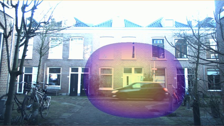
This is the author's version of an article that has been published in this journal. Changes were made to this version by the publisher prior to publication.
                                                      The final version of record is available at           http://dx.doi.org/10.1109/LRA.2021.3062254
2                                                                     IEEE ROBOTICS AND AUTOMATION LETTERS. PREPRINT VERSION. ACCEPTED FEBRUARY, 2021

explored passive acoustic sensing as a sensor for Intelligent                                  labeling [30] or transfer learning [31], since our targets are
Vehicles (IVs). [9], [11], [12] focus on detection and tracking                                visually occluded. Instead, we cast the task as a multi-class
in direct line-of-sight. [13], [14] address detection behind                                   classification problem to identify if and from what corner
corners from a static observer. [13] only shows experiments                                    a vehicle is approaching. We demonstrate that Direction-of-
without directional estimation. [14] tries to accurately model                                 Arrival estimation can provide robust features to classify sound
wave refractions, but experiments in an artificial lab setup                                   reflection patterns, even without end-to-end feature learning
show limited success. Both [13], [14] rely on strong modeling                                  and large amounts of data.
assumptions, ignoring that other informative patterns could                                       Third, for our experiments we collected a new audio-
be present in the acoustic data. Acoustic traffic perception                                   visual dataset in real-world urban environments.1 To collect
is furthermore used for road-side traffic monitoring, e.g. to                                  data, we mounted a front-facing microphone array on our
count vehicles and estimate traffic density [15], [16]. While                                  research vehicle, which additionally has a front-facing camera.
the increase in Electric Vehicles (EVs) may reduce overall                                     This prototype setup facilitates qualitative and quantitative
traffic noise, [17] shows that at 20-30km/h the noise levels for                               experimentation of different acoustic perception tasks.
EV and internal combustion vehicles are already similar due to
tire-road contact. [18] finds that at lower speeds the difference                                                                  III. A PPROACH
is only about 4-5 dB, though many EVs also suffer from
audible narrow peaks in the spectrum. As low speed EVs can                                        Ideally, an ego-vehicle driving through an area with oc-
impact acoustic awareness of humans too [10], legal minimum                                    cluding structures is able to early predict if and from where
sound requirements for EVs are being proposed [19], [20].                                      another vehicle is approaching, even if it is from behind a
   Direction-of-Arrival estimation is a key task for sound                                     blind corner as illustrated in Figure 1. Concretely, this work
source localization, and over the past decades many algorithms                                 aims to distinguish three situations as early as possible using
have been proposed [3], [21], such as the Steered-Response                                     ego-vehicle sensors only:
Power Phase Transform (SRP-PHAT) [22] which is well-suited                                        • an occluded vehicle approaches from behind a corner on
for reverberant environments with possibly distant unknown                                           the left, and only moves into view last-moment when the
sound sources. Still, in urban settings nearby walls, corners,                                       ego-vehicle is about to reach the junction,
and surfaces distort sound signals through reflections and                                        • same, but vehicle approaches behind a right corner,
diffraction [23]. Accounting for such distortions has shown                                       • no vehicle is approaching.
to improve localization [8], [24], but only in controlled indoor                                  We propose to consider this task an online classification
environments where detailed knowledge of the surrounding                                       problem. As the ego-vehicle approaches a blind corner, the
geometry is available.                                                                         acoustic measurements made over short time spans should
   Recently, data-driven methods have shown promising                                          be assigned to one in a set of four classes, C = {left,
results in challenging real-world conditions for various                                       front, right, none}, where left/right indicates a
acoustic tasks. For instance, learned sound models assist                                      still occluded (i.e. not yet in direct line-of-sight) approaching
monaural source separation [25] and source localization from                                   vehicle behind a corner on the left/right, front that the
direction-dependent attenuations by fixed structures [26].                                     vehicle is already in direct line-of-sight, and none that no
Increasingly, deep learning is used for audio classification [27],                             vehicle is approaching.
[28], and localization [29] of sources in line-of-sight, in which                                 In Section III-A we shall first consider two line-of-sight
case visual detectors can replace manual labeling [30], [31].                                  baseline approaches for detecting vehicles. Section III-B then
Analogous to our work, [32] presents a first deep learning                                     elaborates our proposed extension to acoustic non-line-of-sight
method for sensing around corners but with automotive radar.                                   detection. Section III-C provides details of our vehicle’s novel
Thus, while the effect of occlusions on sensor measurements                                    acoustic sensor setup used for data collection.
is difficult to model [14], data-driven approaches appear to
be a good alternative.
                                                                                               A. Line-of-sight detection
   This paper provides the following contributions: First, we                                     We first consider how the task would be addressed with line-
demonstrate in real-world outdoor conditions that a vehicle-                                   of-sight vehicle detection using either conventional cameras,
mounted microphone array can detect the sound of approach-                                     or using past work on acoustic vehicle detection.
ing vehicles behind blind corners from reflections on nearby                                        a) Visual detection baseline: Cameras are currently one
surfaces before line-of-sight detection is feasible. This is a key                             of the de-facto choices for detecting vehicles and other objects
advantage for IVs, where passive acoustic sensing is still rela-                               within line-of-sight. Data-driven Convolutional Neural Net-
tively under-explored. Our experiments investigate the impact                                  works have proven to be highly effective on images. However,
on accuracy and detection time for various conditions, such                                    visual detection can only detect vehicles that are already
as different acoustic environments, driving versus static ego-                                 (partially) visible, and thus only distinguishes between front
vehicle, and compare to current visual and acoustic baselines.                                 and none. To demonstrate this, we use Faster R-CNN [33],
   Second, we propose a data-driven detection pipeline to effi-                                a state-of-the-art visual object detector, on the ego-vehicle’s
ciently address this task and show that it outperforms model-                                  front-facing camera as a visual baseline.
driven acoustic signal processing. Unlike existing data-driven
approaches, we cannot use visual detectors for positional                                         1 Code   & data: github.com/tudelft-iv/occluded vehicle acoustic detection

           Copyright (c) 2021 IEEE. Personal use is permitted. For any other purposes, permission must be obtained from the IEEE by emailing pubs-permissions@ieee.org.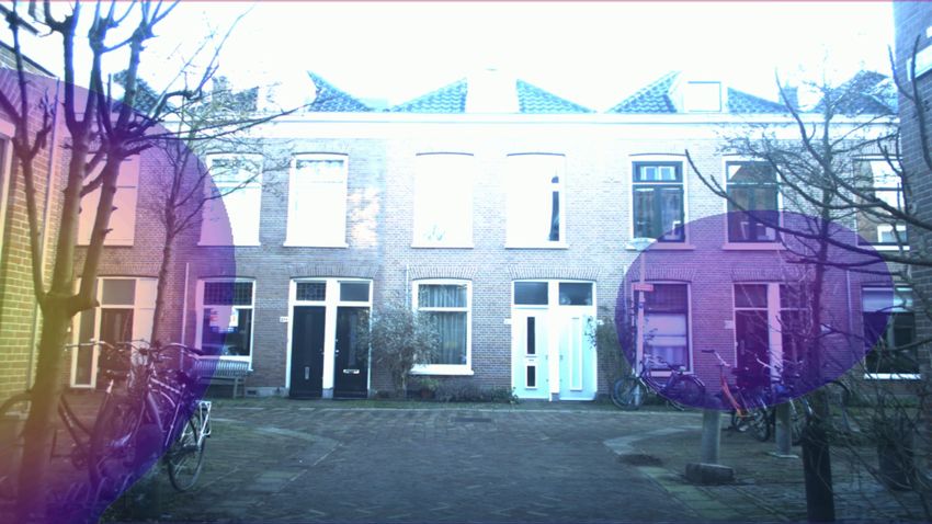
This is the author's version of an article that has been published in this journal. Changes were made to this version by the publisher prior to publication.
The final version of record is available at http://dx.doi.org/10.1109/LRA.2021.3062254
SCHULZ et al.: HEARING WHAT YOU CANNOT SEE 3
Fig. 2. Overview of our acoustic detection pipeline, see Section III-B for an explanation of the steps.
b) Acoustic detection baseline: Next, we consider that through uncontrolled outdoor environments is challenging, es-
the ego-vehicle is equipped with an array of M microphones. pecially as accurate models of the local geometry are missing.
As limited training data hinders learning features (unlike [30], Therefore, we take a data-driven approach and treat the full
[31]), we leverage beamforming to estimate the Direction-of- energy distribution from SRP-PHAT as robust features for our
Arrival (DoA) of tire and engine sounds originating from the classifier that capture all reflections.
approaching vehicle. DoA estimation directly identifies the An overview of the proposed processing pipeline is shown
presence and direction of such sound sources, and has been in Figure 2. We again create M STFTs, using a temporal
shown to work robustly in unoccluded conditions [11], [9]. windows of δt seconds, Hann windowing function and a
Since sounds can be heard around corners, and low frequencies frequency bandpass of [fmin , fmax ] Hz. Notably, we do not
diffract (“bend”) around corners [23], one might wonder: apply any other form of noise filtering or suppression. To
Does the DoA of the sound of an occluded vehicle correctly capture temporal changes in the reflection pattern, we split the
identify from where the vehicle is approaching? To test this STFTs along the temporal dimension into L non-overlapping
hypothesis for our target real-world application, our second segments. For each segment, we compute the DoA energy
baseline follows [11], [9] and directly uses the most salient at multiple azimuth angles α in front of the vehicle. The
DoA angle estimate. azimuth range [−90◦ , +90◦ ] is divided into B equal bins
Specifically, the implementation uses the Steered-Response α1 , · · · , αB . From the original M signals, we thus obtain L
Power-Phase Transform (SRP-PHAT) [22] for DoA estima- response vectors r l = [rl (α1 ), · · · , rl (αB )]> . Finally, these
tion. SRP-PHAT relates the spatial layout of sets of micro- are concatenated to a (L × B)-dimensional feature vector
phone pairs and the temporal offsets of the corresponding x = [r 1 , · · · , r L ]> , for which a Support Vector Machine
audio signals to their relative distance to the sound source. is trained to predict C. Note that increasing the temporal
To apply SRP-PHAT on M continuous synchronized signals, resolution by having more segments L comes at the trade-
only the most recent δt seconds are processed. On each signal, off of a increased final feature vector size and reduced DoA
a Short-Time Fourier Transform (STFT) is computed with a estimation quality due to shorter time windows.
Hann windowing function, and a frequency bandpass for the
[fmin , fmax ] Hz range. Using the generalized cross-correlation C. Acoustic perception research vehicle
of the M STFTs, SRP-PHAT computes the DoA energy r(α)
for any given azimuth angle α around the vehicle. Here α =
−90◦ /0◦ / + 90◦ indicates an angle towards the left/front/right
of the vehicle respectively. If the hypothesis holds that the
overall salient sound direction αmax = arg max r(α) remains A
intact due to diffraction, one only needs to determine if αmax
is beyond some sufficient threshold αth . The baseline thus
assigns class left if αmax < −αth , front if −αth ≤ B
αmax ≤ +αth , and right if αmax > +αth . We shall evaluate
this baseline on the easier task of only separating these three
classes, and ignore the none class.
B. Non-line-of-sight acoustic detection
C
We argue that in contrast to line-of-sight detection, DoA
estimation alone is unsuited for occluded vehicle detection
(and confirm this in Section IV-C). Salient sounds produce
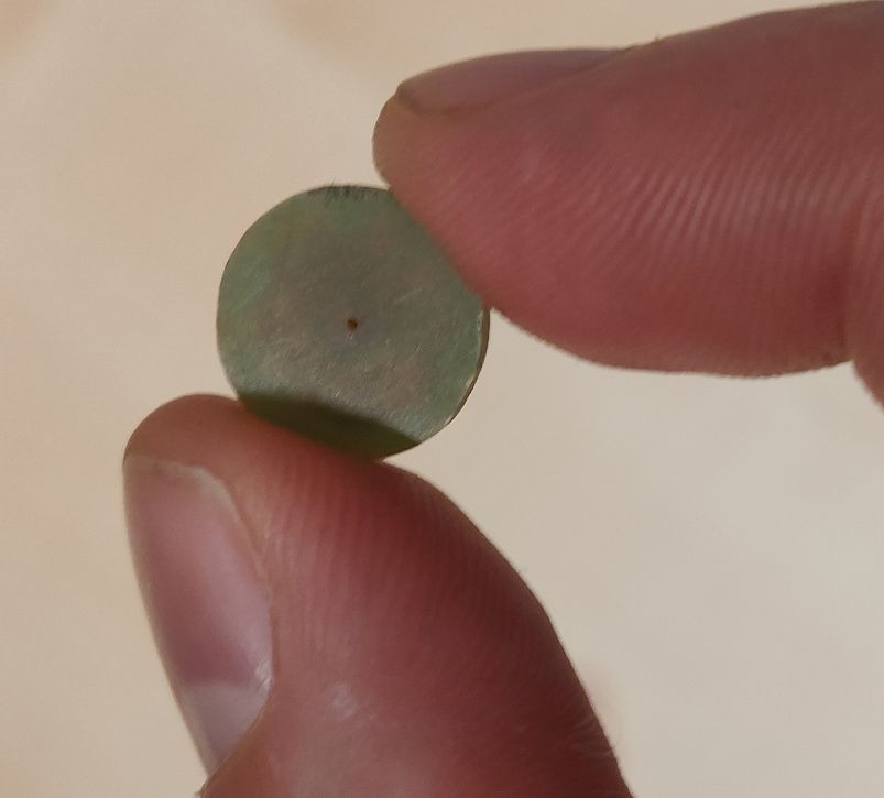
Fig. 3. Sensor setup of our test vehicle. A: Center of the 56 MEMS acoustic
sound wave reflections on surfaces, such as walls (see Figure array. B: signal processing unit. C: front camera behind windscreen. Inset:
1c), thus the DoA does not indicate the actual location of the diameter of a single MEMS microphone is only 12mm.
the source. Modelling the sound propagation [8] while driving
Copyright (c) 2021 IEEE. Personal use is permitted. For any other purposes, permission must be obtained from the IEEE by emailing pubs-permissions@ieee.org.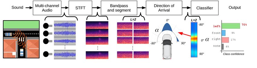
This is the author's version of an article that has been published in this journal. Changes were made to this version by the publisher prior to publication.
The final version of record is available at http://dx.doi.org/10.1109/LRA.2021.3062254
4 IEEE ROBOTICS AND AUTOMATION LETTERS. PREPRINT VERSION. ACCEPTED FEBRUARY, 2021
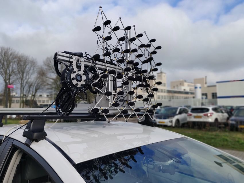
(a) Stroller at a distance (b) Electric scooter (c) Scooter overtaking (d) Car passing by (e) Oncoming car
Fig. 4. Qualitative examples of 2D Direction-of-Arrival estimation overlaid on the camera image (zoomed). (a): Stroller wheels are picked up even at a
distance. (b), (c): Both conventional and more quiet electric scooters are detected. (d): The loudest sound of a passing vehicle is typically the road contact of
the individual tires. (e): Even when the ego-vehicle drives at ∼ 30 km/h, oncoming moving vehicles are still registered as salient sound sources.
To collect real-world data and demonstrate non-line-of- some interesting qualitative findings in real urban conditions.
sight detection, a custom microphone array was mounted on The examples highlight that beamforming can indeed pick
the roof rack of our research vehicle [34], a hybrid electric up various important acoustic events for autonomous driving
Toyota Prius. The microphone array hardware consists of in line-of-sight, such as the presence of vehicles and some
56 ADMP441 MEMS microphones, supports data acquisition vulnerable road users (e.g. strollers). Remarkably, even electric
at 48 kHz sample rate, 24 bits resolution, and synchronous scooters and oncoming traffic while the ego-vehicle is driving
sampling. It was bought from CAE Software & Systems GmbH are recognized as salient sound sources. A key observation
with a metal frame. On this 0.8m × 0.7m frame the micro- from Figure 1c is that sounds originating behind corners reflect
phones are distributed semi-randomly while the microphone in particular patterns on nearby walls. Overall, these results
density remains homogeneous. The general purpose layout was show the feasibility of acoustic detection of (occluded) traffic.
designed by the company through stochastic optimization to
have large variance in inter-microphone distances and serve B. Non-line-of-sight dataset and evaluation metrics
a wide range of acoustic imaging tasks. The vehicle is also
equipped with a front-facing camera for data collection and The quantitative experiments are designed to separately
processing. The center of the microphone array is about 1.78m control and study various factors that could influence acoustic
above the ground, and 0.54m above and 0.50m behind the used perception. We collected multiple recordings of the situations
front camera, see Figure 3. As depicted in the Figure’s inset, explained in Section III at five T-junction locations with blind
the microphones themselves are only 12mm wide. They cost corners in the inner city of Delft. The locations are categorized
about US$1 each. into two types of walled acoustical environments, namely
A signal processing unit receives the analog microphone types A and B (see Figure 5). At these locations common
signals, and sends the data over Ethernet to a PC running the background noise, such as construction sites and other traffic,
Robot Operating System (ROS). Using ROS, the synchronized was present at various volumes. For safety and control, we
microphone signals are collected together with other vehicle did not record in the presence of other motorized traffic on
sensor data. Processing is done in python, using pyroomacous- the roads at the target junction.
tics [21] for acoustic feature extraction, and scikit-learn [35] The recordings can further be divided into Static data, made
for classifier training. while is the ego-vehicle in front of the junction but not moving,
We emphasize that this setup is not intended as a pro- and more challenging Dynamic data where the ego-vehicle
duction prototype, but provides research benefits: The 2D reaches the junction at ∼15 km/h (see the supplementary
planar arrangement provides both horizontal and vertical high- video). Static data is easily collected, and ensures that the
resolution DoA responses, which can be overlaid as 2D main source of variance is the approaching vehicle’s changing
heatmaps [36] on the front camera image to visually study position.
the salient sources (Section IV-A). By testing subsets of
microphones, we can assess the impact of the number of
microphones and their relative placement (Section IV-G). In
-300 00 300 -300 00 300
the future, the array should only use a few microphones at
various locations around the vehicle.
front front
IV. E XPERIMENTS
To validate our method, we created a novel dataset with our
left right left right
acoustic research vehicle in real-world urban environments.
-900 900 -900 900
We first illustrate the quality of acoustic beamforming in such
conditions before turning to our main experiments.
(a) Type A: completely walled (b) Type B: walled exit
A. Line-of-sight localization – qualitative results
Fig. 5. Schematics of considered environment types. The ego-vehicle ap-
As explained in Section III-C, the heatmaps of the 2D DoA proaches the junction from the bottom. Another vehicle might approach behind
results can be overlaid with the camera images. Figure 4 shows the left or right blind corner. Dashed lines indicate the camera FoV.
Copyright (c) 2021 IEEE. Personal use is permitted. For any other purposes, permission must be obtained from the IEEE by emailing pubs-permissions@ieee.org.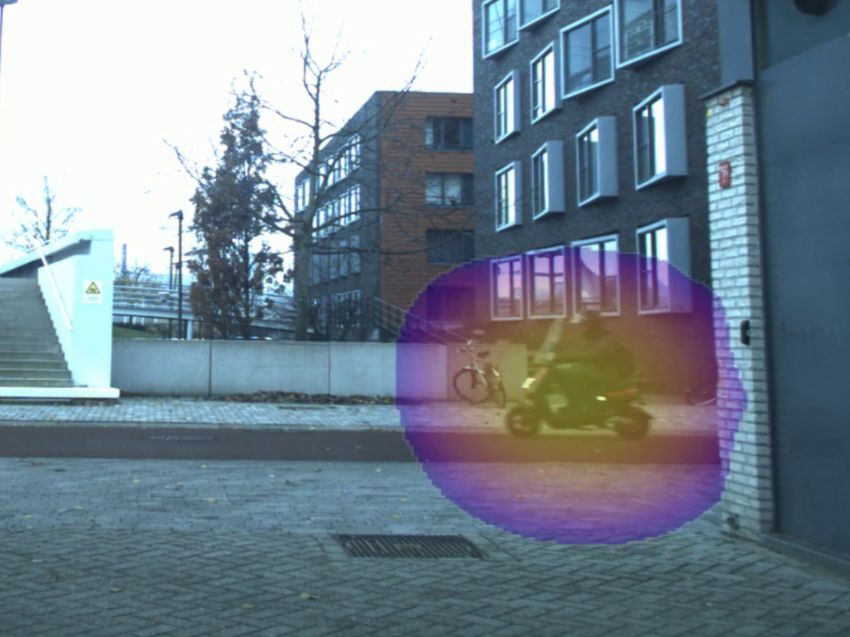
This is the author's version of an article that has been published in this journal. Changes were made to this version by the publisher prior to publication.
                                                      The final version of record is available at           http://dx.doi.org/10.1109/LRA.2021.3062254
SCHULZ et al.: HEARING WHAT YOU CANNOT SEE                                                                                                                                                5

   For the static case, the ego-vehicle was positioned such                                    with no approaching vehicles. Table I lists statistics of the
that the building corners are still visible in the camera and                                  extracted samples at each recording location.
occlude the view onto the intersecting road (on average a                                            b) Data augmentation: Table I shows that the data
distance of ∼7-10m from the intersection). Different types of                                  acquisition scheme produced imbalanced class ratios, with
passing vehicles were recorded, although in most recordings                                    about half the samples for left, right compared to front,
the approaching vehicle was a Škoda Fabia 1.2 TSI (2010)                                      none. Our experiments therefore explore data augmentation.
driven by one of the authors. For the Dynamic case, coor-                                      By exploiting the symmetry of the angular DoA bins, aug-
dinated recordings with the Škoda Fabia were conducted to                                     mentation will double the right and left class samples
ensure that encounters were relevant and executed in a safe                                    by reversing the azimuth bin order in all r l , resulting in new
manner. Situations with left/right/none approaching ve-                                        features for the opposite label, i.e. as if additional data was
hicles were performed in arbitrary order to prevent undesirable                                collected at mirrored locations. Augmentation is a training
correlation of background noise to some class labels. In ∼70%                                  strategy only, and thus not applied to test data to keep results
of the total Dynamic recordings and ∼19.5% of the total Static                                 comparable, and distinct for left and right.
recordings, the ego-vehicle’s noisy internal combustion engine                                       c) Metrics: We report the overall accuracy, and the
was running to charge its battery.                                                             per-class Jaccard index (a.k.a. Intersection-over-Union) as a
                                                                                               robust measure of one-vs-all performance. First, for each
                              TABLE I                                                          class c the True Positives/Negatives (T Pc /T Nc ), and False
  S AMPLES PER SUBSET. I N THE ID, S/D INDICATES S TATIC /DYNAMIC                              Positives/Negatives (F Pc /F Nc ) are computed, treating target
     EGO - VEHICLE , A/B THE ENVIRONMENT TYPE ( SEE FIGURE 5).
                                                                                               class c as positive and the other three classes jointly as
 ID             left         front          right          none            Sum                 negative. Given the P
                                                                                                                   total number of test samples N , the overall
 SA1 / DA1     14 / 19       30 / 38        16 / 19       30 / 37         90/113               accuracy is then      c∈C  T Pc  /N and the per-class Jaccard
 SA2 / DA2     22 / 7        41 / 15        19 / 8        49 / 13        131/ 43               index is Jc = T Pc /(T Pc + F Pc + F Nc ).
 SB1 / DB1     17 / 18       41 / 36        24 / 18       32 / 35        114/107
 SB2 / DB2     28 / 10       55 / 22        27 / 12       43 / 22        153/ 66
 SB3 / DB3     22 / 19       45 / 38        23 / 19       45 / 36        135/112                                           TABLE II
 SAB / DAB     103/ 73       212/149        109/ 76       199/143        623/441                  BASELINE COMPARISON AND HYPERPARAMETER STUDY W. R . T. OUR
                                                                                                   REFERENCE CONFIGURATION : SVM λ = 1, δt = 1, L = 2, DATA
                                                                                                 AUGMENTATION . R ESULTS ON S TATIC DATA . * DENOTES our PIPELINE .
      a) Sample extraction: For each Static recording with an
                                                                                                          Run                   Accuracy         Jleft      Jfront       Jright   Jnone
approaching target vehicle, the time t0 is manually annotated                                        * (reference)                0.92           0.79        0.89         0.87    0.83
as the moment when the approaching vehicle enters direct line-                                   * wo. data augment.              0.92           0.75        0.91         0.78    0.83
of-sight. Since the quality of our t0 estimate is bounded by                                        * w. δt = 0.5s                0.91           0.75        0.89         0.87    0.82
                                                                                                      * w. L = 1                  0.86           0.64        0.87         0.73    0.79
the ego-vehicle’s camera frame rate (10 Hz), we conservatively                                        * w. L = 3                  0.92           0.74        0.92         0.82    0.81
regard the last image before the incoming vehicle is visible as                                       * w. L = 4                  0.90           0.72        0.90         0.77    0.83
t0 . Thus, there is no line-of-sight at t ≤ t0 . At t > t0 the                                   * w. SVM λ = 0.1                 0.91           0.78        0.89         0.81    0.82
                                                                                                  * w. SVM λ = 10                 0.91           0.81        0.86         0.84    0.83
vehicle is considered visible, even though it might only be a                                     DoA-only [11], [9]              0.64           0.11        0.83         0.28      -
fraction of the body. For the Dynamic data, this annotation                                      Faster R-CNN [37]                0.60           0.00        0.99         0.00    0.98
is not feasible as the approaching car may be in direct line-
of-sight, yet outside the limited field-of-view of the front-
facing camera as the ego-vehicle has advanced onto the                                         C. Training and impact of classifier and features
intersection. Thus, annotating t0 based on the camera images is                                   First, the overall system performance and hyperparameters
not representative for line-of-sight detection. To still compare                               are evaluated on all Static data from both type A and B
our results across locations, we manually annotate the time τ0 ,                               locations (i.e. subset ID ‘SAB’) using 5-fold cross-validation.
the moment when the ego-vehicle is at the same position as in                                  The folds are fixed once for all experiments, with the training
the corresponding Static recordings. All Dynamic recordings                                    samples of each class equally distributed among folds.
are aligned to that time as it represents the moment where the                                    We fix the frequency range to fmin = 50Hz, fmax =
ego-vehicle should make a classification decision, irrespective                                1500Hz, and the number of azimuth bins to B = 30 (Section
if an approaching vehicle is about to enter line-of-sight or still                             III-B). For efficiency and robustness, a linear Support Vector
further away.                                                                                  Machine (SVM) is used with l2−regularization weighted by
    From the recordings, short δt = 1s audio samples are                                       hyperparameter λ. Other hyperparameters to explore include
extracted. Let te , the end of the time window [te − 1s, te ],                                 the sample length δt ∈ {0.5s, 1s}, the segment count L ∈
denote a sample’s time stamp at which a prediction could                                       {1, 2, 3, 4}, and using/not using data augmentation.
be made. For Static left and right recordings, samples                                            Our final choice and reference is the SVM with λ = 1,
with the corresponding class label are extracted at te = t0 .                                  δt = 1s, L = 2, and data augmentation. Table II shows
For Dynamic recordings, left and right samples are                                             the results for changing these parameter choices. The overall
extracted at te = τ0 + 0.5s. This ensures that during the 1s                                   accuracy for all these hyperparameters choices is mostly
window the ego-vehicle is on average close to its position                                     similar, though per-class performance does differ. Our refer-
in the Static recordings. In both types of recordings, front                                   ence achieves top accuracy, while also performing well on
samples are extracted 1.5s after the left/right samples,                                       both left and right. We keep its hyperparameters for all
e.g. te = t0 + 1.5s. Class none samples were from recordings                                   following experiments.

           Copyright (c) 2021 IEEE. Personal use is permitted. For any other purposes, permission must be obtained from the IEEE by emailing pubs-permissions@ieee.org.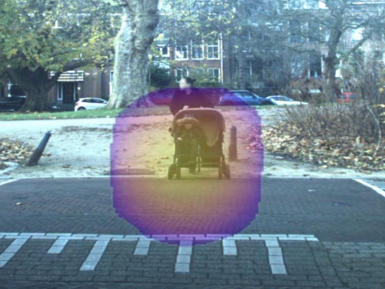
This is the author's version of an article that has been published in this journal. Changes were made to this version by the publisher prior to publication.
                                                                  The final version of record is available at           http://dx.doi.org/10.1109/LRA.2021.3062254
6                                                                                   IEEE ROBOTICS AND AUTOMATION LETTERS. PREPRINT VERSION. ACCEPTED FEBRUARY, 2021

                                                                                                           by the gray area after te = t0 and its beginning thus marks
    −900                                                    α [◦ ]         0°
                                                                                                           when a car enters the field of view. At te = t0 , just before
                                                          -45°                            45°              entering the view of the camera, the approaching car can be
α [◦ ]

              0                                                     αmax          αmax                     detected with 0.94 accuracy by our method. This accuracy is
          0
                                                                                                           achieved more than one second ahead of the visual baseline,
                                                                        NLOS (t0)

         900                                       -90°
                                                                        LOS (t0 + 1.5s)
                                                                                                 90°
                                                                                                           showing that our acoustic detection gives the ego-vehicle
                  -2        0            2            0.3 0.2 0.1
                                                                                                           additional reaction time. After 1.5s a decreasing accuracy is
                         te − t0 [s]                    r(α)
                                                                                                           reported, since the leaving vehicle is not annotated and only
          (a) DoA energy over time                      (b) DoA relative to ego-vehicle
                                                                                                           front predictions are considered true positives. The acoustic
Fig. 6. DoA energy over time for the recording shown in Figure 1c. When                                    detector sometimes still predicts left, or right once the
the approaching vehicle is not in line-of-sight (NLOS), e.g. at t0 , the main
peak is a reflection on the wall (αmax < −30◦ ) opposite of that vehicle.                                  car crossed over. The Faster R-CNN accuracy also decreases:
                                                                                                           after 2s the car is often completely occluded again.
                                                                                                               Figure 8 shows the per-class probabilities as a function
   The table also shows the results of the DoA-only baseline                                               of extraction time te on the test set, separated by recording
explained in Section III-A using αth = 50◦ , which was found                                               situations. The SVM class probabilities are obtained with the
through a grid search in the range [0◦ , 90◦ ]. As expected, the                                           method in [38]. The probabilities for left show that on
DoA-only baseline [11], [9] shows weak performance for all                                                 average the model initially predicts that no car is approaching.
metrics. While the sound source is occluded, the most salient                                              Towards t0 , the none class becomes less likely and the model
sound direction does not represent its origin, but its reflection                                          increasingly favors the correct left class. A short time after
on the opposite wall (see Figure 1). The temporal evolution of                                             t0 , the prediction flips to the front class, and eventually
the full DoA energy for a car approaching from the right                                                   switches to right as the car leaves line-of-sight. Similar
is shown in Figure 6. When it is still occluded at t0 , there                                              (mirrored) behavior is observed for vehicles approaching from
are multiple peaks and the most salient one is a reflection on                                             the right. The probabilities of left/right rise until the ap-
the left (αmax ≈ −40◦ ). Only once the car is in line-of-sight                                             proaching vehicle is almost in line-of-sight, which corresponds
(t0 + 1.5s) the main mode clearly represents its true direction                                            to the extraction time of the training samples. The none
(αmax ≈ +25◦ ). The left and right image in Figure 1c also                                                 class is constantly predicted as likeliest when no vehicle is
show such peaks at t0 and t0 + 1.5s, respectively.                                                         approaching. Overall, the prediction matches the events of the
   The bottom row of the table shows the visual baseline, a                                                recorded situations remarkably well.
Faster R-CNN R50-C4 model trained on the COCO dataset
[37]. To avoid false positive detections, we set the score
threshold of 75% and additionally required a bounding box
                                                                                                           Accuracy

height of 100 pixels to ignore cars far away in the background,
which were not of interest. Generally this threshold is already
exceeded once the hood of the approaching car is visible.
While performing well on front and none, this visual base-
line shows poor overall accuracy as it is physically incapable
of classifying left and right.                                                                                                                       te − t0 [s]
                                                                                                           Fig. 7. Accuracy over test time te of our acoustic and the visual baseline on
D. Detection time before appearance                                                                        83 Static recordings. Gray region indicates the other vehicle is half-occluded
                                                                                                           and two labels, front and either left or right, are considered correct.
   Ultimately, the goal is to know whether our acoustic method
can detect approaching vehicles earlier than the state-of-the-
art visual baseline. For this purpose, their online performance                                                                              TABLE III
is compared next.                                                                                                C ROSS - VALIDATION RESULTS PER ENVIRONMENT ON DYNAMIC DATA .
   The static recordings are divided into a fixed training                                                             Subset       Accuracy         Jleft      Jfront       Jright       Jnone
(328 recordings) and test (83 recordings) split, stratified to                                                          DAB           0.76           0.41        0.80         0.44        0.65
adequately represent labels and locations. The training was                                                             DA            0.84           0.66        0.85         0.64        0.72
                                                                                                                         DB           0.75           0.33        0.81         0.42        0.64
conducted as in Section IV-C with left and right samples
extracted at te = t0 . The visual baseline is evaluated on every
camera frame (10 Hz). Our detector is evaluated on a sliding
window of 1s across the 83 test recordings. To account for the                                             E. Impact of the moving ego-vehicle
transition period when the car may still be partly occluded,                                                  Next, our classifier is evaluated by cross-validation per
front predictions by both methods are accepted as correct                                                  environment subset, as well as on the full Dynamic data. As
starting at t = t0 . For recordings of classes left and right,                                             for the Static data, 5-fold cross-validation is applied to each
these classes are accepted until t = t0 + 1.5s, allowing for                                               subset, keeping the class distribution balanced across folds.
temporal overlap with front.                                                                                  Table III lists the corresponding metrics for each subset.
   Figure 7 illustrates the accuracy on the test recordings for                                            On the full Dynamic data (DAB), the accuracy indicates
different evaluation times te . The overlap region is indicated                                            decent performance, but the metrics for left and right

                       Copyright (c) 2021 IEEE. Personal use is permitted. For any other purposes, permission must be obtained from the IEEE by emailing pubs-permissions@ieee.org.
This is the author's version of an article that has been published in this journal. Changes were made to this version by the publisher prior to publication.
The final version of record is available at http://dx.doi.org/10.1109/LRA.2021.3062254
SCHULZ et al.: HEARING WHAT YOU CANNOT SEE 7
1.0 1.0 1.0
front left none right
0.8 0.8 0.8
p(c|x)
0.6 0.6 0.6
0.4 0.4 0.4
0.2 0.2 0.2
0.0 0.0 0.0
−6 −4 −2 0 2 −6 −4 −2 0 2 −6 −4 −2 0 2
te − t0 [s] te − t0 [s] te − t0 [s]
(a) left recordings (b) right recordings (c) none recordings
Fig. 8. Mean and std. dev. of predicted class probabilities at different times te on test set recordings of the Static data (blue is front, green is left, red
is right, and black is none). Each figure shows recordings of a different situation. The approaching vehicle appears in view just after te − t0 = 0.
F. Generalization across acoustic environments
1.0 1.0
0.8 0.8
We here study how the performance is affected when the
p(c|x)
0.6 0.6
classifier is trained on all samples from one environment type
0.4 0.4
and evaluated on all samples of the other type. In Table IV,
0.2 0.2 combinations of training and test sets are listed. Compared
0.0 0.0 to the results for Static and Dynamic data (see Tables II and
−6 −4 −2 0 2 −6 −4 −2 0 2
te − τ0 [s] te − τ0 [s] III), the reported results in the table show a general trend:
(a) left recordings (b) right recordings If the classifier is trained on one environment and tested on
Fig. 9. Mean and std. dev. of predicted class probabilities at different times te
the other, it performs worse than when samples of the same
on left and right test set recordings of the Dynamic data. The ego-vehicle location are used. In particular, the classifier trained on SB
reached the location of training data when te − τ0 = 0.5s. and tested on SA is not able to correctly classify samples of
left and right while inverse training and testing performs
much better. On the Dynamic data, such pronounced effects
are not visible, but overall the accuracy decreases compared to
classes are much worse compared to the Static results in the Static data. In summary, the reflection patterns vary from
Table II. Separating subsets DA and DB reveals that the one environment to another, yet at some locations the patterns
performance is highly dependent on the environment type. In appear more distinct and robust than those at others.
fact, even with limited training data and large data variance
from a driving ego-vehicle, we obtain decent classification TABLE IV
performance on type A environments, and we notice that low G ENERALIZATION ACROSS LOCATIONS AND ENVIRONMENTS .
left and right performance mainly results from type B
Training Test Accuracy Jleft Jfront Jright Jnone
environments. We hypothesize that the more confined type A SB SA 0.66 0.03 0.66 0.03 0.62
environments reflect more target sounds and are better shielded SA SB 0.79 0.42 0.82 0.61 0.67
from potential noise sources. DB DA 0.53 0.16 0.70 0.25 0.16
DA DB 0.56 0.21 0.50 0.29 0.46
We also analyze the temporal behavior of our method on
Dynamic data. Unfortunately, a fair comparison with a visual
baseline is not possible: the ego-vehicle often reaches the G. Microphone array configuration
intersection early, and the approaching vehicle is within line-
of-sight but still outside the front-facing camera’s field of view Our array with 56 microphones enables evaluation of differ-
(cf. τ0 extraction in Section IV-B). Yet, the evolution of the ent spatial configurations with M < 56. For various subsets of
56
predicted probabilities can be compared to those on the Static M microphones, we randomly sample 100 out of M possible
data in Section IV-D. Figure 9 illustrates the average predicted microphone configurations, and cross-validate on the Static
probabilities over 59 Dynamic test set recordings from all data. Interestingly, the best configuration with M = 7 already
locations, after training on samples from the remaining 233 achieves similar accuracy as with M = 56. With M = 2/3 the
recordings. The classifier on average correctly predicts right accuracy is already 0.82/0.89, but with worse performance on
samples (Figure 9b), between te = τ0 to te = τ0 +0.5s. Of the left and right. Large variance between samples highlights
left recordings at these times, many are falsely predicted as the importance of a thorough search of spatial configurations.
none, only few are confused with right. Furthermore, the Reducing M also leads to faster inference time, specifically
changing ego-perspective of the vehicle results in alternating 0.24/0.14/0.04s for M = 56/28/14 using our unoptimized
DoA-energy directions and thus class predictions, compared to implementation.
the Static results in Figure 8. This indicates that it might help
to include the ego-vehicle’s relative position as an additional V. C ONCLUSIONS
feature, and obtain more varied training data to cover the We showed that a vehicle mounted microphone array can be
positional variations. used to acoustically detect approaching vehicles behind blind
Copyright (c) 2021 IEEE. Personal use is permitted. For any other purposes, permission must be obtained from the IEEE by emailing pubs-permissions@ieee.org.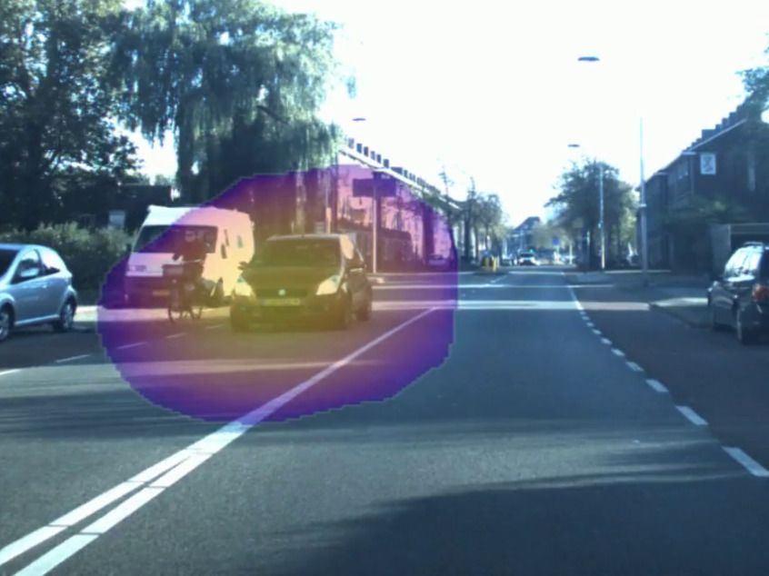
This is the author's version of an article that has been published in this journal. Changes were made to this version by the publisher prior to publication.
                                                         The final version of record is available at           http://dx.doi.org/10.1109/LRA.2021.3062254
8                                                                        IEEE ROBOTICS AND AUTOMATION LETTERS. PREPRINT VERSION. ACCEPTED FEBRUARY, 2021

corners from their wall reflections. In our experimental setup,                                   [15] T. Toyoda, N. Ono, S. Miyabe, T. Yamada, and S. Makino, “Traffic
our method achieved an accuracy of 0.92 on the 4-class hidden                                          monitoring with ad-hoc microphone array,” in Int. Workshop on Acoustic
                                                                                                       Signal Enhancement. IEEE, 2014, pp. 318–322.
car classification task for a static ego-vehicle, and up to 0.84                                  [16] S. Ishida, J. Kajimura, M. Uchino, S. Tagashira, and A. Fukuda,
in some environments while driving. An approaching vehicle                                             “SAVeD: Acoustic vehicle detector with speed estimation capable of
was detected with the same accuracy as our visual baseline                                             sequential vehicle detection,” in ITSC. IEEE, 2018, pp. 906–912.
                                                                                                  [17] U. Sandberg, L. Goubert, and P. Mioduszewski, “Are vehicles driven in
already more than one second ahead, a crucial advantage in                                             electric mode so quiet that they need acoustic warning signals,” in Int.
such critical situations.                                                                              Congress on Acoustics, 2010.
   While these initial findings are encouraging, our results                                      [18] L. M. Iversen and R. S. H. Skov, “Measurement of noise from electrical
                                                                                                       vehicles and internal combustion engine vehicles under urban driving
have several limitations. The experiments included only few                                            conditions,” Euronoise, 2015.
locations and few different oncoming vehicles, and while our                                      [19] R. Robart, E. Parizet, J.-C. Chamard, et al., “eVADER: A perceptual
method performed well on one environment, it had difficulties                                          approach to finding minimum warning sound requirements for quiet
                                                                                                       cars.” in AIA-DAGA 2013 Conference on Acoustics, 2013.
on the other, and did not perform reliably in unseen test                                         [20] S. K. Lee, S. M. Lee, T. Shin, and M. Han, “Objective evaluation
environments. To expand the applicability, we expect that more                                         of the sound quality of the warning sound of electric vehicles with a
representative data is needed to capture a broad variety of en-                                        consideration of the masking effect: Annoyance and detectability,” Int.
                                                                                                       Journal of Automotive Tech., vol. 18, no. 4, pp. 699–705, 2017.
vironments, vehicle positions and velocities, and the presence                                    [21] R. Scheibler, E. Bezzam, and I. Dokmanić, “Pyroomacoustics: A python
of multiple sound sources. Rather than generalizing across                                             package for audio room simulation and array processing algorithms,” in
environments, additional input from map data or other sensor                                           ICASSP. IEEE, 2018, pp. 351–355.
                                                                                                  [22] J. H. DiBiase, A high-accuracy, low-latency technique for talker local-
measurements could help to discriminate acoustic environ-                                              ization in reverberant environments using microphone arrays. Brown
ments and to classify the reflection patterns accordingly. More                                        University Providence, RI, 2000.
data also enables end-to-end learning of low-level features,                                      [23] M. Hornikx and J. Forssén, “Modelling of sound propagation to three-
                                                                                                       dimensional urban courtyards using the extended Fourier pstd method,”
potentially capturing cues our DoA-based approach currently                                            Applied Acoustics, vol. 72, no. 9, pp. 665–676, 2011.
ignores (e.g. Doppler, sound volume), and perform multi-                                          [24] W. Zhang, P. N. Samarasinghe, H. Chen, and T. D. Abhayapala, “Sur-
source detection and classification in one pass [30]. Ideally                                          round by sound: A review of spatial audio recording and reproduction,”
                                                                                                       Applied Sciences, vol. 7, no. 5, p. 532, 2017.
a suitable self-supervised learning scheme is developed [31],                                     [25] K. Osako, Y. Mitsufuji, et al., “Supervised monaural source separation
though a key challenge is that actual occluded sources cannot                                          based on autoencoders,” in ICASSP. IEEE, 2017, pp. 11–15.
immediately be visually detected.                                                                 [26] A. Saxena and A. Y. Ng, “Learning sound location from a single
                                                                                                       microphone,” in ICRA. IEEE, 2009, pp. 1737–1742.
                                                                                                  [27] J. Salamon and J. P. Bello, “Deep convolutional neural networks and
                                                                                                       data augmentation for environmental sound classification,” IEEE Signal
                                 R EFERENCES                                                           Processing Letters, vol. 24, no. 3, pp. 279–283, 2017.
                                                                                                  [28] A. Valada, L. Spinello, and W. Burgard, “Deep feature learning for
 [1] C. G. Keller, T. Dang, H. Fritz, A. Joos, C. Rabe, and D. M. Gavrila,                             acoustics-based terrain classification,” in Robotics Research. Springer,
     “Active pedestrian safety by automatic braking and evasive steering,”                             2018, pp. 21–37.
     IEEE T-ITS, vol. 12, no. 4, pp. 1292–1304, 2011.                                             [29] N. Yalta, K. Nakadai, and T. Ogata, “Sound source localization using
 [2] Z. MacHardy, A. Khan, K. Obana, and S. Iwashina, “V2X access                                      deep learning models,” J. of Robotics and Mechatronics, vol. 29, no. 1,
     technologies: Regulation, research, and remaining challenges,” IEEE                               pp. 37–48, 2017.
     Comm. Surveys & Tutorials, vol. 20, no. 3, pp. 1858–1877, 2018.                              [30] W. He, P. Motlicek, and J.-M. Odobez, “Deep neural networks for
 [3] S. Argentieri, P. Danes, and P. Souères, “A survey on sound source                               multiple speaker detection and localization,” in ICRA. IEEE, 2018,
     localization in robotics: From binaural to array processing methods,”                             pp. 74–79.
     Computer Speech & Language, vol. 34, no. 1, pp. 87–112, 2015.                                [31] C. Gan, H. Zhao, P. Chen, D. Cox, and A. Torralba, “Self-supervised
 [4] C. Rascon and I. Meza, “Localization of sound sources in robotics: A                              moving vehicle tracking with stereo sound,” in Proc. of ICCV, 2019.
     review,” Robotics & Autonomous Systems, vol. 96, pp. 184–210, 2017.                          [32] N. Scheiner, F. Kraus, F. Wei, et al., “Seeing around street corners: Non-
 [5] L. Wang and A. Cavallaro, “Acoustic sensing from a multi-rotor drone,”                            line-of-sight detection and tracking in-the-wild using doppler radar,” in
     IEEE Sensors Journal, vol. 18, no. 11, pp. 4570–4582, 2018.                                       Proc. of IEEE CVPR, 2020, pp. 2068–2077.
 [6] D. B. Lindell, G. Wetzstein, and V. Koltun, “Acoustic non-line-of-sight                      [33] S. Ren, K. He, R. Girshick, and J. Sun, “Faster r-cnn: Towards real-time
     imaging,” in Proc. of IEEE CVPR, 2019, pp. 6780–6789.                                             object detection with region proposal networks,” in Advances in neural
 [7] K. Okutani, T. Yoshida, K. Nakamura, and K. Nakadai, “Outdoor                                     information processing systems, 2015, pp. 91–99.
     auditory scene analysis using a moving microphone array embedded                             [34] L. Ferranti, B. Brito, E. Pool, Y. Zheng, et al., “SafeVRU: A research
     in a quadrocopter,” in IEEE/RSJ IROS. IEEE, 2012, pp. 3288–3293.                                  platform for the interaction of self-driving vehicles with vulnerable road
 [8] I. An, M. Son, D. Manocha, and S.-e. Yoon, “Reflection-aware sound                                users,” in IV Symposium. IEEE, 2019, pp. 1660–1666.
     source localization,” in ICRA. IEEE, 2018, pp. 66–73.                                        [35] F. Pedregosa, G. Varoquaux, et al., “Scikit-learn: Machine learning in
 [9] Y. Jang, J. Kim, and J. Kim, “The development of the vehicle sound                                python,” JMLR, vol. 12, no. Oct, pp. 2825–2830, 2011.
     source localization system,” in APSIPA. IEEE, 2015, pp. 1241–1244.                           [36] E. Sarradj and G. Herold, “A python framework for microphone array
[10] A. Stelling-Kończak, M. Hagenzieker, and B. V. Wee, “Traffic sounds                              data processing,” Applied Acoustics, vol. 116, pp. 50–58, 2017.
     and cycling safety: The use of electronic devices by cyclists and the                        [37] Y. Wu, A. Kirillov, F. Massa, W.-Y. Lo, and R. Girshick, “Detectron2,”
     quietness of hybrid and electric cars,” Transport Reviews, vol. 35, no. 4,                        https://github.com/facebookresearch/detectron2, 2019.
     pp. 422–444, 2015.                                                                           [38] T.-F. Wu, C.-J. Lin, and R. C. Weng, “Probability estimates for multi-
[11] M. Mizumachi, A. Kaminuma, N. Ono, and S. Ando, “Robust sensing of                                class classification by pairwise coupling,” JMLR, vol. 5, no. Aug, pp.
     approaching vehicles relying on acoustic cues,” Sensors, vol. 14, no. 6,                          975–1005, 2004.
     pp. 9546–9561, 2014.
[12] A. V. Padmanabhan, H. Ravichandran, et al., “Acoustics based vehicle
     environmental information,” SAE, Tech. Rep., 2014.
[13] K. Asahi, H. Banno, O. Yamamoto, A. Ogawa, and K. Yamada, “Devel-
     opment and evaluation of a scheme for detecting multiple approaching
     vehicles through acoustic sensing,” in IV Symposium. IEEE, 2011, pp.
     119–123.
[14] V. Singh, K. E. Knisely, et al., “Non-line-of-sight sound source local-
     ization using matched-field processing,” J. of the Acoustical Society of
     America, vol. 131, no. 1, pp. 292–302, 2012.

              Copyright (c) 2021 IEEE. Personal use is permitted. For any other purposes, permission must be obtained from the IEEE by emailing pubs-permissions@ieee.org.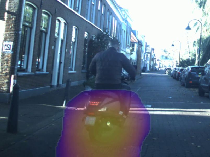
You can also read