Using Georeferenced Twitter Data to Estimate Pedestrian Traffic in an Urban Road Network - DROPS
←
→
Page content transcription
If your browser does not render page correctly, please read the page content below
Using Georeferenced Twitter Data to Estimate
Pedestrian Traffic in an Urban Road Network
Debjit Bhowmick1
Department of Infrastructure Engineering, The University of Melbourne, Australia
dbhowmick@student.unimelb.edu.au

Stephan Winter
Department of Infrastructure Engineering, The University of Melbourne, Australia
winter@unimelb.edu.au

Mark Stevenson
Melbourne School of Design, Department of Infrastructure Engineering, The University of
Melbourne, Australia
mark.stevenson@unimelb.edu.au

        Abstract
Since existing methods to estimate the pedestrian activity in an urban area are data-intensive,
we ask the question whether just georeferenced Twitter data can be a viable proxy for inferring
pedestrian activity. Walking is often the mode of the last leg reaching an activity location, from
where, presumably, the tweets originate. This study analyses this question in three steps. First, we
use correlation analysis to assess whether georeferenced Twitter data can be used as a viable proxy
for inferring pedestrian activity. Then we adopt standard regression analysis to estimate pedestrian
traffic at existing pedestrian sensor locations using georeferenced tweets alone. Thirdly, exploiting
the results above, we estimate the hourly pedestrian traffic counts at every segment of the study area
network for every hour of every day of the week. Results show a fair correlation between tweets and
pedestrian counts, in contrast to counts of other modes of travelling. Thus, this method contributes
a non-data-intensive approach for estimating pedestrian activity. Since Twitter is an omnipresent,
publicly available data source, this study transcends the boundaries of geographic transferability
and scalability, unlike its more traditional counterparts.

2012 ACM Subject Classification Information systems → Geographic information systems

Keywords and phrases Twitter, pedestrian traffic, location-based, regression analysis, correlation
analysis

Digital Object Identifier 10.4230/LIPIcs.GIScience.2021.I.1

    1    Introduction

1.1      Background and motivation
Urban traffic monitoring and analysis is increasingly important with the ever-growing urban
population. Urban traffic consists of two major modes of travel, namely the vehicular mode
(automobile, bicycle, transit) and the pedestrian mode [38]. Research on urban vehicular
traffic has been popular for the past five or six decades owing to increased number of motorised
vehicles on the road and the consequent challenges related to traffic congestion, competition
for space and consumption of resources. On the contrary, the focus on pedestrians is more
recent with the authorities now spending more resources on developing infrastructure for
active mobility (non-motorised forms of transport such as biking and walking) to curb the
detrimental impact of the motorised modes on public health and climate.

1
    Corresponding author
            © Debjit Bhowmick, Stephan Winter, and Mark Stevenson;
            licensed under Creative Commons License CC-BY
11th International Conference on Geographic Information Science (GIScience 2021) – Part I.
Editors: Krzysztof Janowicz and Judith A. Verstegen; Article No. 1; pp. 1:1–1:15
                   Leibniz International Proceedings in Informatics
                   Schloss Dagstuhl – Leibniz-Zentrum für Informatik, Dagstuhl Publishing, Germany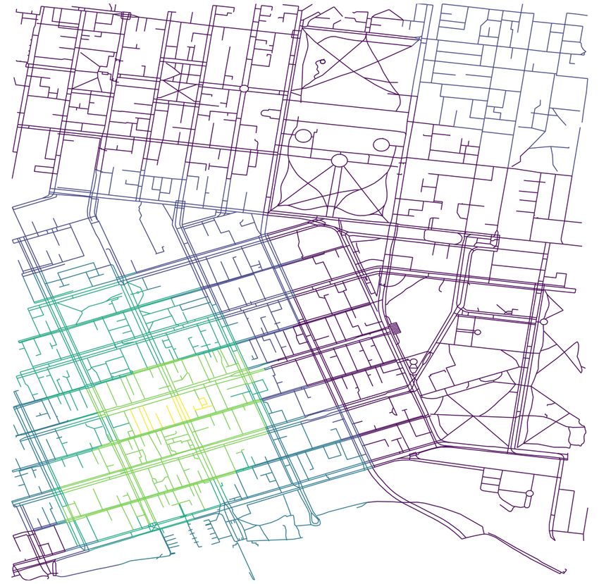
1:2   Using Twitter Data to Estimate Pedestrian Traffic

          While walking is the most common and essential travel mode as almost all places are
      accessible on foot [39, 13], several studies have shown the benefits of walking with respect to
      a person’s physical and mental health [3, 18, 14]. On a larger scale, walking generates indirect
      public health benefits by reducing the use of automobiles, consequently reducing traffic
      congestion, energy consumption, air and noise pollution, the overall level of traffic danger,
      and thus offerring more liveable communities [26, 37]. Besides public health, pedestrian
      activity is an important factor in urban planning, transportation management and decisions
      affecting land use and real estate. Analytical insights on pedestrian activity assists governing
      authorities to estimate demand with greater accuracy and allocate resources accordingly,
      which, in turn, improves operations.
          Owing to the late rise in popularity of research relating to the pedestrian mode (being
      overlooked for decades), datasets representing pedestrian activity and movement are limited
      as compared to its motorised counterparts, more so in developing nations. As a result, most
      studies are still based on the traditional data collection methods of questionnaire surveys,
      manual counting, and tracking people’s movements using GPS devices and smartphones
      [25, 2, 31, 9, 30, 5, 27]. While these methods are effective, they involve significant monetary
      costs and suffer from the issues of scalability and transferability in both space and time.
      Moreover, some of these forms of data collection such as GPS tracking, are highly privacy-
      sensitive [17]. On the other hand, traditional pedestrian volume estimation studies [22, 31, 9]
      are dependent on multiple, highly localised, predictor datasets which are not available in
      most places . Hence, there is a growing necessity for cheap, publicly available, omnipresent
      proxy data which transcends the boundaries of scalability and transferability. In this regard,
      location-based social media data, especially Twitter, has gained increasing attention by
      researchers who have used it to tackle a host of real-world problems including the detection
      and prediction of vehicular traffic levels [32], unusual levels of vehicular traffic congestion,
      accidents and disruptions [10, 8, 35], pedestrian congestion [34] and crowd movements at
      various spatio-temporal scales [7, 4].

      1.2    Related work
      There is limited systematic research comparing the nature of association of location-based
      social media data with varying urban travel modes to investigate the possibility that some
      modes are better represented by such data as compared to the others. While [32] have
      shown that Twitter and Instagram data can be used as a predictor for actual vehicular traffic
      by using Odds Ratio, Risk Ratio and RT-DBSCAN, the nature of association was drawn
      from comparing only the abnormalities of social media distribution and vehicular traffic
      volume. Since their work intends to identify traffic congestion in near-real time, their methods
      are limited to successfully differentiating between normal and anomalous traffic volumes.
      Although [7] and [4] have predicted crowd flow using Twitter, their study is also limited to
      outlier detection and anomalous behaviour resulting from events. On the other hand, [34]
      predicted pedestrian congestion using georeferenced tweet counts but did neither report any
      validation, nor any evidence of association between tweets and pedestrian congestion in the
      first place. In contrast to the aforementioned literature, this study investigates the possibility
      of using georeferenced tweets as a viable proxy for predicting pedestrian traffic and shows
      how tweet counts can be used for prediction of pedestrian traffic at high spatio-temporal
      resolution.
          Other studies have used more traditional approaches of estimating pedestrian traffic at
      locations by quantifying the influence of multiple predictor variables. [22] presented a model
      to estimate the pedestrian volumes for street intersections. The study found that population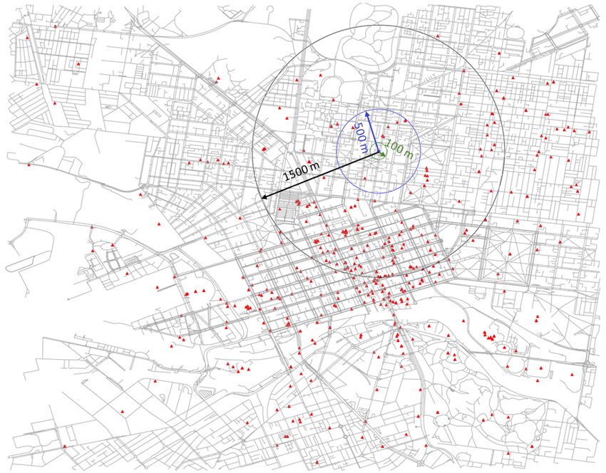
D. Bhowmick, S. Winter, and M. Stevenson                                                                1:3

and job density, local transit access, and land use mix had the strongest explanatory power on
variances of pedestrian volume. [31] used a log-linear regression model to identify statistically
significant relationships between annual pedestrian volume at road intersections and predictor
variables such as land use, transportation system, local environment and socio-economic
characteristics surrounding the intersections. Similarly, [9] proposed a scalable approach by
using regression models to predict pedestrian volume at road intersections using multiple
infrastructural datasets and extrapolate at locations where count data was absent. All these
studies are highly data-intensive and are dependent on the spatio-temporal granularity of
the datasets representing the explanatory variables.
    Among other techniques, the space syntax tool is stands out for being less data-intensive
and relying only on street network data [11]. While this configurational approach has been
used to predict pedestrian movement to an acceptable extent (roughly 60%) [21] in urban
spaces, it is well-studied and has a well-developed methodology. But, existing literature has
not employed social media data, or even investigated, in the first place, whether it can be
used as a measure of estimating the number of pedestrians at a given location at a given time
period. On the contrary, this study proposes a novel approach which is not only a scalable,
but also transferable and non-data intensive by only using publicly available georeferenced
Twitter data with fine granularity instead of employing multiple datasets.

1.3    Research hypothesis and objectives
This study aims to prove the hypothesis that georeferenced Twitter traffic can be used as a
viable proxy for estimating pedestrian counts under specific conditions of space and time,
with a certain degree of accuracy. The objectives of this paper are:
1. To show the existence of a strong positive correlation between georeferenced Twitter
    traffic and pedestrian traffic and that this correlation is stronger than vehicular traffic,
2. To develop a scalable and transferable method that predicts pedestrian traffic with
    reasonable accuracy, at any location in an urban network using only georeferenced tweet
    counts with high spatial and temporal granularity.
To attain the stated objectives, this study makes use of publicly available georeferenced
Twitter data, pedestrian count data made available by the City of Melbourne, and vehicular
traffic data from SCATS made available by the Victorian Government.
    Overall, the contributions of this study are three-fold.
1. In the first step, this study implements correlation analysis to understand the association
    between georeferenced Twitter traffic and two major urban travel modes, pedestrian
    and vehicular traffic, by looking at the nature of correlations and the spatio-temporal
    patterns of variation of correlation. It compares the results across the two travel modes
    to understand whether one mode is more strongly associated with georeferenced tweets
    under certain conditions of space-time and hence tweets can be inferred as a viable proxy
    for that mode.
2. Based on the findings from the first step, which reveals the existence of a relatively stronger
    and more statistically significant correlation between Twitter traffic and pedestrian traffic
    as compared to vehicular traffic, the second step of this study uses standard regression
    analysis to estimate pedestrian traffic and the resultant estimation errors at existing
    pedestrian sensor locations, at any given hour of any day of the week. The method is
    geographically transferable and is able to estimate pedestrian traffic at the finest level of
    spatial granularity.
3. In the final step, this study predicts pedestrian traffic at every segment of the study area
    network (even where pedestrian counts are not available) at hourly intervals of any given
    date using georeferenced tweet counts.

                                                                                                     GIScience 2021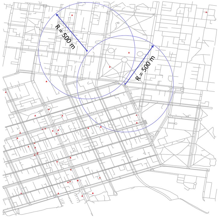
1:4   Using Twitter Data to Estimate Pedestrian Traffic

       2      Data overview

      2.1     Pedestrian counts dataset
      The City of Melbourne had developed an automated pedestrian counting system in 2009 to
      better understand pedestrian activity within the municipality. Using non-vision based sensors
      installed at multiple strategic locations in its administrative area (covering the Central
      Business District and its neighbouring suburbs), it collects counts of pedestrians on an hourly
      basis. The open dataset contains hourly pedestrian counts since 2009 and is updated on a
      monthly basis. The dataset is structured with the following information:
      1. Sensor ID
      2. Sensor location (street name)
      3. Coordinates of sensor location (latitude, longitude)
      4. Hourly pedestrian count
       5. Detailed timestamp (date, day of the week, hour of the day)
      During the period of data collection for this study (January to April 2018) there were 49
      active sensor locations in the city. Figure 1 shows the locations of the pedestrian sensors
      (blue markers).

           Figure 1 Locations of pedestrian sensors (blue) and SCATS sensors (red) in the City of Melbourne.

      2.2     Vehicular counts dataset
      The official source of the vehicle count data for the cities in Australia is based on the
      Sydney Coordinated Adaptive Traffic System (SCATS, www.scats.com.au). Recordings are
      made at intervals of 15 minutes and are available for download from the VicRoads website
      (www.vicroads.gov.au). Hourly vehicular traffic for each of the 45 sensor locations in terms
      of counts of vehicles were collected for the period of March 2018. Figure 1 shows the locations
      of the pedestrian sensors (red markers).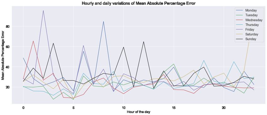
D. Bhowmick, S. Winter, and M. Stevenson                                                             1:5

2.3    Twitter dataset

The Australian Urban Research Infrastructure Network (AURIN, www.aurin.org.au) has
harvested tweets originating from all major cities of Australia from July 2014 to May
2018 using Twitter’s Public Streaming API which allows for a real-time collection of a
random sample of tweets. The collection of tweets was not continuous as the dataset
contains significant time gaps (April to July 2015, March 2016, May 2016 to May 2017).
Similar to previous studies conducted in the domain of spatial information using Twitter
data, this research will rely only on precisely georeferenced tweets (tweets with explicit
latitude/longitude information). In 2019, Twitter has turned off the option of precise
georeferencing. Since then georeferenced tweets provide location information usually in terms
of places of varying granularity. These coarse georeferences are also user selected, and hence
there is no guarantee whether they were posted in that place at all. For this study, however,
we rely on the precise georeferences which are system-generated and hence reliable. [24]
compared the data from the Streaming API and the Firehose data set (the complete set of
tweets available commercially) and stated that the 1% sample provided by the Streaming
API almost returns the complete set of precisely georeferenced tweets despite the sampling.
The challenge with the small number of precisely georeferenced tweets is that they only
represent a set of self-selecting individuals supplying volunteered data. Thus they are highly
unlikely to be representative of the entire pedestrian population of the study area. Regardless
of this major caveat, it is accepted best practice in the literature to base investigations on
this selective data. For this study of predicting pedestrian traffic, even if the tweets are
non-representative, the base assumption of a correlation between persons’ tweeting and their
participation at activities still holds.

2.4    Study settings

The area chosen for this study is the City of Melbourne, one of the 32 local councils making
up Greater Melbourne. City of Melbourne covers an area of roughly 37 km2 and consists of
metropolitan Melbourne’s innermost suburbs, including the central business district. The
study area includes an area specified by a bounding box, judiciously chosen to cover all
sensor locations of the city’s pedestrian counting system with adequate buffer zones. The
coordinates of the bounding box are (-37.8359, 144.9269, -37.7860, 144.9903).
    Since the Twitter dataset contains periods of gaps, this study makes use of the most recent
and continuous time span for which the data was collected, from January 2018 to April 2018.
Using the bounding box coordinates specified while defining the study area, 28197 precisely
georeferenced tweets (a subset of the 10 million tweets extracted by AURIN in Greater
Melbourne during the study period) were obtained for the study period. As this study aims
to compare and investigate the nature of associations between pedestrian counts (which are
relatively large numbers in the study area) and tweet counts (which are comparatively small
numbers), any relationship between the two is highly sensitive. To avoid any further bias,
we filtered out any consecutive tweets of the same user in our chosen time intervals, hence,
counting Twitter users rather than tweets in each 1-hour period. Furthermore, tweeting
activity was observed to be anomalous during 1st January and hence, it was removed from
the dataset. This resulted in the final dataset of 25679 precisely georeferenced tweets.

                                                                                                  GIScience 2021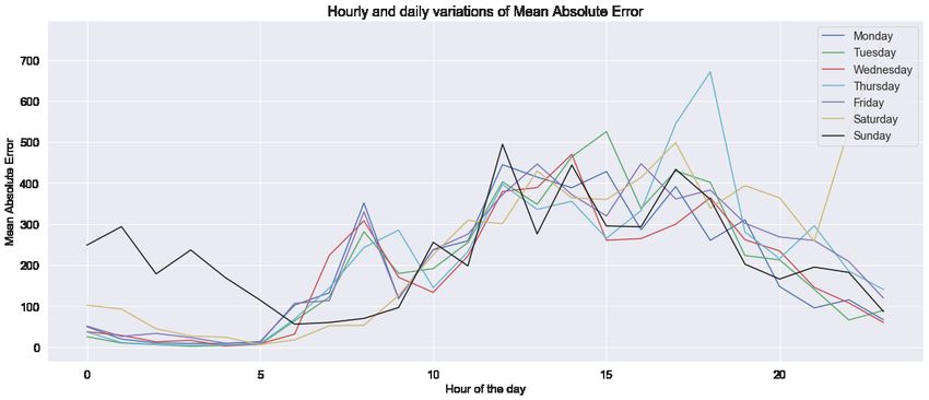
1:6   Using Twitter Data to Estimate Pedestrian Traffic

       3     Correlation analysis between tweet counts and pedestrian counts

      The underlying assumption of this experiment is that highly populated outdoor spaces have
      a greater probability of experiencing high tweet counts, and in turn, high georeferenced tweet
      counts, than places with lower populations. This is in line with existing literature where
      social media has been used as proxy measure for urban land use [6], urban activity spaces
      [19, 23], ambient population [12], and most importantly pedestrian population [34, 7, 4].
      While details of these studies [34, 7, 4] have been discussed in Section 1, all of them have
      assumed the latent existence of an association between tweets and pedestrians. This study
      bases its hypothesis on such findings and ventures deeper to investigate whether georeferenced
      Twitter data can actually be used as a viable proxy for inferring pedestrian traffic in an
      urban area. Since pedestrian count data is the most accurate representation of pedestrian
      traffic at a given location, this study aims to infer to what extent these counts are correlated
      with the count of georeferenced tweets. Additionally, this study makes use of vehicular traffic
      data obtained from SCATS locations to draw comparisons between pedestrian and vehicular
      travel mode in terms of the strength of correlation. It compares the results of the analyses
      across the two travel modes to understand whether georeferenced tweets can be inferred as a
      viable proxy for urban pedestrian traffic.
           Using the location information of the active pedestrian sensors, an imaginary circular
      buffer (catchment) area was drawn with a sensor at the centre of a circle. Similar spatial
      querying was conducted before by [22] and [15, 16] in their studies of predicting pedestrian
      volume across intersections in San Francisco and New York City respectively. This spatial
      querying was performed to capture the number of precisely georeferenced tweets. The radius
      of the circle was varied from 100 to 1500 metres in steps of 100 metres. Using point-in-polygon
      analysis, each tweet was assigned to the pedestrian counter(s) in whose catchment area it
      fell. Correlation was drawn between the observed pedestrian count in each sensor and tweet
      count inside the catchment area of the same sensor, both at hourly and daily time intervals.
      For the vehicular traffic data, the SCATS location nearest to each pedestrian sensor was
      considered as the centre of a catchment circle and correlation was computed for the month
      of March 2018 only. A sample illustration of the aforementioned method has been shown in
      Figure 2.
          The results of the correlation analysis between georeferenced tweet counts and pedestrian
      counts are shown in Figure 3. It can be observed that there exists a clear hourly pattern
      in the variation of correlation coefficient, while the daily pattern is less prominent. The
      resultant magnitude of correlation coefficients reduces drastically in between 5 AM to 10 AM,
      while remaining relatively high and statistically significant for the rest of the day. This could
      be attributed to the fact that Twitter traffic starts increasing more rapidly after 7 AM and
      reaches its peak quicker than pedestrian traffic, as observed from Twitter data of Melbourne
      (shown in Figure 4) and Australia [20]. Another possible cause could be that streets that are
      busy during those times do not cater to a lot of Twitter traffic (pedestrians not tweeting on
      busy streets before starting work). This indicates that pedestrian activities that are more
      tweet-productive, are found to be happening before 5 AM and after 10 AM. As far as days of
      week are concerned, weekends exhibit a slightly improved positive correlation coefficient value
      than weekdays. This maybe again attributed to the fact that weekend activities (which are
      more interesting) are more tweet-productive than weekday activities and that tweet counts
      are more reflective of actual pedestrian counts at places.
         Also, the correlation coefficient varies significantly with the radius of the catchment
      area. It can be observed in Figure 3 that the correlation coefficient gradually increases with
      the increase in the radius of the circular catchment area, reaching its peak at 500 metres.
D. Bhowmick, S. Winter, and M. Stevenson 1:7
Figure 2 Spatial querying for georeferenced tweets made between 10 AM and 11 AM inside the
study area (red triangular markers) using a circular buffer with radius 100, 500 and 1500 metres for
a randomly chosen sensor (blue round marker).
Interestingly, about 500 metres is the average walking range [1, 29, 33, 36, 28]. It then starts
to reduce: Larger catchment areas lead to overlaps of catchment areas, and of tweets counted
multiple times, thereby reducing the effectiveness of our experiment. The least correlation
was observed at 1500 metres radius.
On the other hand, the association between vehicular traffic and georeferenced Twitter
traffic appears to be substantially weaker. As shown in Figure 5, the magnitude of the
resultant correlation coefficients is relatively less as compared to the ones obtained from
pedestrian counts. Also, most of the coefficients are not statistically significant at 95%
confidence level. This comparison throws up anticipated and intuitive results. It is more
likely that tweets are made during a pedestrian activity as compared to a driving activity
as walking is often the final mode of reaching an activity location, from where, presumably,
the tweets originate. The results reaffirm this likelihood. Although there exists no binding
definition of what a pedestrian activity exactly means (or is limited to), the general consensus
is that it usually spans more than just the period of walking itself. On the contrary, vehicular
activity is more limited and is confined to only driving a vehicle or being a passenger in one.
While this experiment was aimed more at inferring correlation as opposed to causation
(which cannot be proven even with a statistically significant correlation coefficient), it adds
the aspect of novelty to this study by establishing the correlation, its magnitude and temporal
patterns, before proceeding to use tweets to measure pedestrian activity. Also, explanations
can be speculated by observing fair correlations which helps in hypothesis generation. Hence,
based on these findings, this study now argues with conviction that georeferenced tweet
counts may be used as a viable proxy for estimating pedestrian count under given conditions.
The following section aims at calculating errors arising while estimating pedestrian traffic
from georeferenced tweet counts.
GIScience 20211:8 Using Twitter Data to Estimate Pedestrian Traffic
(a) With radius of catchment circle and hour of the day
(b) With radius of catchment circle and day of the week
Figure 3 Variation of correlation coefficient (georeferenced tweet counts and pedestrian counts);
dark blue points indicate the correlation is statistically significant at 95% confidence level.
4 Estimating pedestrian counts at existing sensor locations
Based on the findings from the first stage of this study, the second stage proposes to use
standard regression analysis to estimate pedestrian traffic using tweet counts. It aims to
investigate the one-to-one relationship between georeferenced tweet counts and pedestrian
counts. It describes, in detail, the methodology of handling the dataset and computing the
resultant errors obtained during estimation of pedestrian counts via regression in terms of
common regression metrics such as Mean Absolute Error (MAE) and Mean Absolute Percent-
age Error (MAPE). The only predictor variable used in regression is precisely georeferenced
tweet count.
Using georeferenced tweet counts as the predictor variable (on the x-axis), an attempt
was made to replicate its relationship with pedestrian counts, which is the predicted variable
(on the y-axis). For this purpose, standard regression modelling was employed. For each hour
of each day of the week (e.g., Thursday 1500 hours), a unique regression curve was developed,
thus resulting in a total of 168 curves (24 hours multiplied by 7 days). Since this study
is the first to investigate such one-to-one relationship between georeferenced tweet counts
and pedestrian counts, it was made sure that the chosen regression model is comparatively
better (in terms of standard regression metrics) and logical (non-overfitting) at the same
time. Hence, trial regression analyses were performed using linear, log-linear, quadraticD. Bhowmick, S. Winter, and M. Stevenson 1:9
(a) Hourly variation in pedestrian (b) Hourly variation in vehicular (c) Hourly variation in georefer-
count count enced tweet count
Figure 4 Variation in the City of Melbourne: (a) hourly pedestrian count per sensor, (b) hourly
vehicular count per sensor and (b) aggregate hourly tweet count.
and cubic models. Previous studies related to pedestrian count prediction have used either
linear or log-linear models to test statistical relationship between walkability measures and
pedestrian volume [31, 15, 16]. Although these models have lesser accuracy, these models do
not completely contradict this global behaviour, and hence either could be accepted as a
viable representation. Quadratic and cubic models exhibited lesser errors but were prone to
overfitting, and hence were not considered. The results of the regression analyses are shown
in Table 1. Mean hourly values of the regression metrics (R-squared, MAE and MAPE) are
obtained by taking arithmetic means of metric values over 168 cases (every hour of every day
of the week). The temporal variation of the regression metrics have been shown in Figure 6.
Table 1 Regression metrics for January-April 2018.
Regression x-axis y-axis Mean Mean Mean
model hourly hourly hourly
R-squared MAE MAPE
Linear Georeferenced Pedestrian 0.426 192.6 28.3
tweet count count
Log-linear loge (Georeferenced Pedestrian 0.424 212.9 26.9
tweet count) count
The performance of the mean hourly tweet count - mean hourly pedestrian count regression
curves obtained from this study were tested by applying the method to predict mean
pedestrian counts of a different time period. For this purpose, data from November 2017
was chosen as it was the nearest month available from our study period devoid of known
anomalies. They exhibit slightly greater estimation errors (linear: MAE = 274.3, MAPE
= 35.83 and log-linear: MAE = 292.0, MAPE = 34.43), which could be due to seasonal
variations in the tweet count - pedestrian count relationship that was not taken into account
due to absence of continuous tweet collection periods. Nevertheless, the errors and temporal
patterns are similar to the ones shown in Table 1 and Figure 6 respectively. Hence, the
regression curves obtained in this study are acceptable.
GIScience 20211:10 Using Twitter Data to Estimate Pedestrian Traffic
(a) With radius of catchment circle and hour of the day
(b) With radius of catchment circle and day of the week
Figure 5 Variation of correlation coefficient (georeferenced tweet counts and vehicular counts);
dark blue points indicate the correlation is statistically significant at 95% confidence level.
5 Predicting pedestrian counts at locations without any pedestrian
count information
The third and final stage of this study is aimed at extrapolation of the developed methodology.
The intention to develop a transferable (temporally and spatially) and scalable pedestrian
count prediction methodology was based on the motive to predict pedestrian counts at high
temporal (hour of the day of the week) and spatial resolution (point on the urban road
network), even at locations without any pedestrian count information. The following method
helps in predicting the pedestrian counts at any point in an urban pedestrian road network,
given the date and time (at hourly granularity).
Pedestrian network data was obtained from OpenStreetMap using the bounding box
coordinates specified in Section 2.4. For a given hour of any given date, georeferenced
tweets were extracted from the AURIN dataset. Consequently, iterating over all edges of the
network, centered on the mid point of an edge spatial querying was conducted using a 500
metre search radius to extract the number of georeferenced tweets. These tweet counts were
associated with the corresponding edge. After obtaining the information on the queried hour
of the day and day of the week , iterating over all edges of the network, the corresponding
regression curve was referred to estimate the pedestrian count passing through an edge.
A sample illustration of the spatial querying process to estimate pedestrian counts using
georeferenced tweet counts for January 2, 2018 during 1000 to 1100 hours and the resultant
estimation of pedestrian counts have been shown in Figure 7.D. Bhowmick, S. Winter, and M. Stevenson 1:11
(a) Variation of MAE using linear regression with hour of the day and day of the week
(b) Variation of MAPE using linear regression with hour of the day and day of the week
Figure 6 Temporal patterns of regression metrics.
6 Discussion
The three stages of analysis reported in this study makes novel contributions by finding
moderate to high correlations between georeferenced tweet counts and pedestrian counts, and
then developing a scalable, transferable and non-data-intensive methodology for estimating
pedestrian counts from georeferenced tweet counts. Finally, using spatial querying, the study
predicted pedestrian counts at high temporal and spatial resolution at locations devoid of
sensors. Yet there are limitations of this study that need to be highlighted as well.
First, it was observed in Section 3 that the values of the resultant correlation coefficients
during 5 AM to 10 AM were relatively lower in magnitude and statistically insignificant.
Hence, predictions using regression curves during this time period are expected to be more
erroneous. This is apparent from Figure 6 where the MAE and MAPE can be observed to
reach high values (higher than the mean) during this time period, in most of the days. It
can be argued that this time period is not ideal for making pedestrian volume prediction
using georeferenced tweet counts alone.
Results in Section 4 showed that the proposed methodology produces significant estimation
errors in both the study dataset as well as in the testing dataset. While this study argues
about the benefits of employing a non-data-intensive approach to predict pedestrian counts in
Section 1.2, the magnitude of errors indicate the drawbacks. The regression curve generalises
GIScience 20211:12 Using Twitter Data to Estimate Pedestrian Traffic
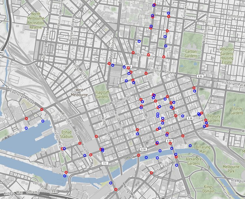
(a) Spatial querying for tweets (red trian- (b) Edges of the network labelled as per
gular markers) using a circular buffer with predicted pedestrian counts. Lighter colours
radius 500 metres for 2 randomly chosen edge (yellow, green) indicate higher pedestrian
mid points (blue round markers) volume, while darker colours (blue, purple)
indicate lower pedestrian volume
Figure 7 Prediction of pedestrian counts using precisely georeferenced tweet counts by extrapola-
tion during 1000 to 1100 hours on January 2, 2018.
all network segments with zero georeferenced tweet count as having one and the same
pedestrian volume equal to the intercept of the regression curve, which overestimates the
actual pedestrian volume in most cases. Furthermore, the betweenness centrality of the
edges of the network was calculated to tally the results with the pedestrian count predictions.
The dead ends, for example, have zero betweenness centrality but, it can be observed from
Figure 7 that the proposed method is not differentiating between through roads and dead
ends, in terms of pedestrian counts. These challenges will be addressed in a future study
by analysing other network attributes (data-intensive) such as road width, road hierarchy,
proximity to transit stops, number of Points-of-Interest which are proven factors known to
influence pedestrian demand, to produce more representative results.
The underlying assumption of this study was that the entire study area is homogeneous
in terms of every spatial attribute, apart from the spatial distribution of georeferenced
tweets. Thus it assumed a existing one-to-one relationship between georeferenced tweet
counts and pedestrian counts that varies temporally, but not spatially. The argument in
favour of this assumption is that this study was conducted in a relatively homogeneous area
in terms of land use. But the results indicate that this assumption is not robust, and there
are multiple possible reasons. The relationship between georeferenced tweet counts and
pedestrian counts is not independent of spatial variables. Different locations have different
tweet count - pedestrian count relationships depending on location type. For example, the
tweet productiveness of a railway station is possibly different from the tweet productiveness of
an event location, both in magnitude and in temporal patterns. While both may experience
pedestrian counts to the same degree, it is expected that an event will bring out greater
number of georeferenced tweets than the lesser interesting public transit, for the same number
of pedestrian counts. Hence, future work will address this shortcoming by incorporating the
spatial variation of the relationship between tweet productivity and land use.D. Bhowmick, S. Winter, and M. Stevenson 1:13
Finally, it must be noted that Twitter has removed the support for precise georeferencing
of tweets since June 2019. Thus, the proposed method is applicable only on historic datasets.
In terms of estimating pedestrian counts, this move impacts on any real-time interests, but
long-term averages should not change quickly. To mitigate this, time-series modelling using
historic tweet counts can be applied to predict future tweet counts, which can be used for
predicting pedestrian counts using the same principle in future scenarios.
7 Conclusion and future work
Despite the highlighted limitations, this study contributes novel insights. The three-step
methodology remains transferable due to use of an omnipresent data source. It can be applied
if acceptable correlations are achieved. However, the regression equations in our case study
will not hold true for another study area and need to be re-calculated for a different study
area. Also, the size of the study area can be increased or decreased without any change in the
methodology, with intuitive variations in estimation accuracy. Yet, analysis at micro-level
and homogeneous land-use will need some strict assumptions. Also, a study area that is too
small will have fewer geotagged tweets. Lastly, we attempted to mitigate population disparity
between indoor spaces and adjoining outdoor spaces. We made justifiable assumptions that
populated indoor spaces indicate popularity in its adjoining outdoor space, given a space-time
buffer. Thus, we placed a 1-hour time buffer and a 500m radius distance buffer around
pedestrian counters to capture tweets. We assume to catch most of the tweets and pedestrians
in the same buffer although some exceptions will always be there. This uncertainty flattens
out as the study area grows in size. Not only does this study investigate the nature of existing
correlation, but also proposes an approach to estimate pedestrian counts from georeferenced
tweet counts, even at places devoid of pedestrian sensors. By doing so, this study shows the
extent to which this non-data-intensive approach can predict pedestrian counts (in terms of
estimation errors) and thus brings out the limitations of such an approach, which need to be
addressed in future to achieve more accurate and representative results.
References
1 V Thamizh Arasan, VR Rengaraju, and KV Krishna Rao. Characteristics of trips by foot and
bicycle modes in Indian city. Journal of Transportation Engineering, 120(2):283–294, 1994.
2 Hieronymus C Borst, Sanne I de Vries, Jamie MA Graham, Jef EF van Dongen, Ingrid Bakker,
and Henk ME Miedema. Influence of environmental street characteristics on walking route
choice of elderly people. Journal of Environmental Psychology, 29(4):477–484, 2009.
3 JE Donnelly, DJ Jacobsen, K Snyder Heelan, R Seip, and S Smith. The effects of 18 months
of intermittent vs continuous exercise on aerobic capacity, body weight and composition, and
metabolic fitness in previously sedentary, moderately obese females. International Journal of
Obesity, 24(5):566, 2000.
4 Ana Fernández Vilas, Rebeca P Díaz Redondo, and Mohamed Ben Khalifa. Analysis of crowds’
movement using Twitter. Computational Intelligence, 35(2):448–472, 2019.
5 Sheila Ferrer and Tomás Ruiz. The impact of the built environment on the decision to walk
for short trips: Evidence from two Spanish cities. Transport Policy, 67:111–120, 2018.
6 Vanessa Frias-Martinez and Enrique Frias-Martinez. Spectral clustering for sensing urban
land use using Twitter activity. Engineering Applications of Artificial Intelligence, 35:237–245,
2014.
7 Gary Goh, Jing Yu Koh, and Yue Zhang. Twitter-informed crowd flow prediction. In 2018
IEEE International Conference on Data Mining Workshops (ICDMW), pages 624–631. IEEE,
2018.
GIScience 20211:14 Using Twitter Data to Estimate Pedestrian Traffic
8 Yikai Gong, Fengmin Deng, and Richard O Sinnott. Identification of (near) Real-time Traffic
Congestion in the Cities of Australia through Twitter. In Proceedings of the ACM First
International Workshop on Understanding the City with Urban Informatics, pages 7–12. ACM,
2015.
9 Amir Hajrasouliha and Li Yin. The impact of street network connectivity on pedestrian
volume. Urban Studies, 52(13):2483–2497, 2015.
10 Jingrui He, Wei Shen, Phani Divakaruni, Laura Wynter, and Rick Lawrence. Improving
traffic prediction with tweet semantics. In 23rd International Joint Conference on Artificial
Intelligence, pages 1387–1393, 2013.
11 Bill Hillier, Alan Penn, Julienne Hanson, Tadeusz Grajewski, and Jianming Xu. Natural
Movement: or, Configuration and Attraction in Urban Pedestrian Movement. Environment
and Planning B: planning and design, 20(1):29–66, 1993.
12 John R Hipp, Christopher Bates, Moshe Lichman, and Padhraic Smyth. Using Social Media
to Measure Temporal Ambient Population: Does it Help Explain Local Crime Rates? Justice
Quarterly, 36(4):718–748, 2019.
13 Jinhyun Hong and Cynthia Chen. The role of the built environment on perceived safety from
crime and walking: Examining direct and indirect impacts. Transportation, 41(6):1171–1185,
2014.
14 Marcus Johansson, Terry Hartig, and Henk Staats. Psychological benefits of walking: Mod-
eration by company and outdoor environment. Applied Psychology: Health and Well-Being,
3(3):261–280, 2011. doi:10.1111/j.1758-0854.2011.01051.x.
15 Yuan Lai and Constantine Kontokosta. Analyzing the Drivers of Pedestrian Activity at
High Spatial Resolution. In 2017 International Conference on Sustainable Infrastructure:
Methodology, ICSI 2017, pages 303–314. American Society of Civil Engineers (ASCE), 2017.
16 Yuan Lai and Constantine E Kontokosta. Quantifying place: Analyzing the drivers of pedestrian
activity in dense urban environments. Landscape and Urban Planning, 180:166–178, 2018.
17 J. K. Laurila, Daniel Gatica-Perez, I. Aad, Blom J., Olivier Bornet, Trinh-Minh-Tri Do,
O. Dousse, J. Eberle, and M. Miettinen. The Mobile Data Challenge: Big Data for Mobile
Computing Research. Infoscience : EPFL Scientific Publications, 2012.
18 I-Min Lee and David M Buchner. The importance of walking to public health. Medicine &
Science in Sports and Exercise, 40(7 Suppl):S512–8, 2008.
19 Jae Hyun Lee, Adam W Davis, Seo Youn Yoon, and Konstadinos G Goulias. Activity
Space Estimation with Longitudinal Observations of Social Media Data. Transportation,
43(6):955–977, 2016.
20 Kevan Lee. The Biggest Social Media Science Study: What 4.8 Million Tweets
Say About the Best Time to Tweet, 2016. URL: https://buffer.com/resources/
best-time-to-tweet-research.
21 Yoav Lerman, Yodan Rofè, and Itzhak Omer. Using Space Syntax to Model Pedestrian
Movement in Urban Transportation Planning. Geographical Analysis, 46(4):392–410, 2014.
22 XiaoHang Liu and Julia Griswold. Pedestrian volume modeling: A case study of San Francisco.
Yearbook of the Association of Pacific Coast Geographers, pages 164–181, 2009.
23 Nick Malleson and Mark Birkin. New insights into individual activity spaces using crowd-
sourced big data. In 2014 ASE BigData/SocialCom/CyberSecurity Conference, Stanford
University. Academy of Science and Engineering (ASE), USA, 2014.
24 Fred Morstatter, Jürgen Pfeffer, Huan Liu, and Kathleen M Carley. Is the sample good
enough? Comparing data from Twitter’s streaming api with Twitter’s Firehose. In Seventh
International AAAI Conference on Weblogs and Social Media, 2013.
25 J Michael Oakes, Ann Forsyth, and Kathryn H Schmitz. The effects of neighborhood density
and street connectivity on walking behavior: The twin cities walking study. Epidemiologic
Perspectives & Innovations, 4(1):16, 2007.
26 John Pucher and Ralph Buehler. Walking and cycling for healthy cities. Built Environment,
36(4):391–414, 2010.D. Bhowmick, S. Winter, and M. Stevenson 1:15
27 LSC Pun-Cheng and CWY So. A comparative analysis of perceived and actual walking
behaviour in varying land use and time. Journal of Location Based Services, pages 1–20, 2019.
28 TM Rahul and Ashish Verma. A study of acceptable trip distances using walking and cycling
in Bangalore. Journal of Transport Geography, 38:106–113, 2014.
29 S. Robertson. Usability of pedestrian crossings: Further results from fieldwork Contemporary
Ergonomics 2005. Taylor & Francis, 2005.
30 Daniel A Rodríguez, Louis Merlin, Carlo G Prato, Terry L Conway, Deborah Cohen, John P
Elder, Kelly R Evenson, Thomas L McKenzie, Julie L Pickrel, and Sara Veblen-Mortenson.
Influence of the built environment on pedestrian route choices of adolescent girls. Environment
and Behavior, 47(4):359–394, 2015.
31 Robert J Schneider, Todd Henry, Meghan F Mitman, Laura Stonehill, and Jesse Koehler.
Development and Application of Volume Model for Pedestrian Intersections in San Francisco,
California. Transportation Research Record, 2299(1):65–78, 2012.
32 Richard O Sinnott, Yikai Gong, Shiping Chen, and Paul Rimba. Urban traffic analysis using
social media data on the cloud. In 2018 IEEE/ACM International Conference on Utility and
Cloud Computing Companion (UCC Companion), pages 134–141. IEEE, 2018.
33 State of Victoria. Pedestrian access strategy : A strategy to increase walking for transport in
Victoria. Technical report, State of Victoria, 2010.
34 Shoko Wakamiya, Yukiko Kawai, Hiroshi Kawasaki, Ryong Lee, Kazutoshi Sumiya, and
Toyokazu Akiyama. Crowd-sourced prediction of pedestrian congestion for bike navigation
systems. In 5th ACM SIGSPATIAL International Workshop on GeoStreaming, pages 25–32.
Association for Computing Machinery, Inc, 2014.
35 S. Wongcharoen and T. Senivongse. Twitter analysis of road traffic congestion severity
estimation. In 2016 13th International Joint Conference on Computer Science and Software
Engineering (JCSSE), page 6 pp. IEEE, 2016.
36 Yong Yang and Ana V Diez-Roux. Walking distance by trip purpose and population subgroups.
American Journal of Preventive Medicine, 43(1):11–19, 2012.
37 Xuan Zhang and Lan Mu. The perceived importance and objective measurement of walkability
in the built environment rating. Environment and Planning B: Urban Analytics and City
Science, page 2399808319832305, 2019.
38 Yinan Zheng, Lily Elefteriadou, Thomas Chase, Bastian Schroeder, and Virginia Sisiopiku.
Pedestrian Traffic Operations in Urban Networks. Transportation Research Procedia, 15:137–
149, 2016.
39 Dennis Zielstra and Hartwig Hochmair. Using free and proprietary data to compare shortest-
path lengths for effective pedestrian routing in street networks. Transportation Research
Record: Journal of the Transportation Research Board, 2299(1):41–47, 2012.
GIScience 2021You can also read