Probabilistic Sensor Fusion for Ambient Assisted Living
←
→
Page content transcription
If your browser does not render page correctly, please read the page content below
Probabilistic Sensor Fusion for Ambient Assisted Living
                                                        Tom Diethea,∗, Niall Twomeya , Meelis Kulla , Peter Flacha , Ian Craddocka
                                                                        a
                                                                            Intelligent Systems Laboratory, University of Bristol

                                          Abstract
                                          There is a widely-accepted need to revise current forms of health-care provision, with particular
                                          interest in sensing systems in the home. Given a multiple-modality sensor platform with hetero-
arXiv:1702.01209v1 [stat.ML] 4 Feb 2017

                                          geneous network connectivity, as is under development in the Sensor Platform for HEalthcare
                                          in Residential Environment (SPHERE) Interdisciplinary Research Collaboration (IRC), we face
                                          specific challenges relating to the fusion of the heterogeneous sensor modalities.
                                               We introduce Bayesian models for sensor fusion, which aims to address the challenges of
                                          fusion of heterogeneous sensor modalities. Using this approach we are able to identify the modal-
                                          ities that have most utility for each particular activity, and simultaneously identify which features
                                          within that activity are most relevant for a given activity.
                                               We further show how the two separate tasks of location prediction and activity recognition can
                                          be fused into a single model, which allows for simultaneous learning an prediction for both tasks.
                                               We analyse the performance of this model on data collected in the SPHERE house, and show
                                          its utility. We also compare against some benchmark models which do not have the full structure,
                                          and show how the proposed model compares favourably to these methods.
                                          Keywords: Bayesian, Sensor Fusion, Smart Homes, Ambient Assisted Living

                                          1. Introduction
                                          1.1. Ambient and Assisted Living
                                              Due to well-known demographic challenges, traditional regimes of health-care are in need
                                          of re-examination. Many countries are experiencing the effects of an ageing population, which
                                          coupled with a rise in chronic health conditions is expediting a shift towards the management of
                                          a wide variety of health related issues in the home. In this context, advances in Ambient Assisted
                                          Living (AAL) are providing resources to improve the experience of patients, as well as informing
                                          necessary interventions from relatives, carers and health-care professionals.

                                             ∗
                                              I am corresponding author
                                              Email addresses: tom.diethe@bristol.ac.uk (Tom Diethe), niall.twomey@bristol.ac.uk
                                          (Niall Twomey), meelis.kull@bristol.ac.uk (Meelis Kull), peter.flach@bristol.ac.uk (Peter
                                          Flach), ian.craddock@bristol.ac.uk (Ian Craddock)
                                              URL: www.tomdiethe.com (Tom Diethe)

                                          Preprint submitted to Information Fusion                                                  February 7, 2017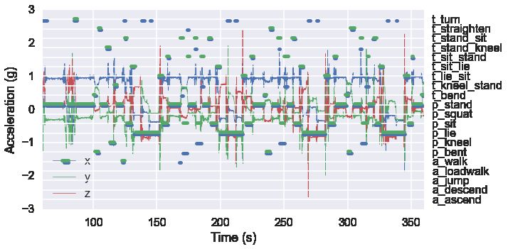
To this end the EPSRC-funded “Sensor Platform for HEalthcare in Residential Environment
(SPHERE)” Interdisciplinary Research Collaboration (IRC) [9, 26, 27, 25] has designed a multi-
modal system driven by data analytics requirements. The system is under test in a single house,
and deployment to a general population of 100 homes in Bristol (UK) is underway at the time of
writing. Wherever possible, the data collected will be made available to researchers in a variety of
communities.
    Data fusion and machine learning in this setting is required to address two main challenges:
transparent decision making under uncertainty; and adapting to multiple operating contexts. Here
we focus on the first of these challenges, by describing an approach to sensor fusions that takes a
principled approach to the quantification of uncertainty whilst maintaining the ability to introspect
on the decisions being made.

1.2. Quantification of Uncertainty
    Multiple heterogeneous sensors in a real world environment introduce different sources of
uncertainty. At a basic level, we might have sensors that are simply not working, or that are giving
incorrect readings. More generally, a given sensor will at any given time have a particular signal
to noise ratio, and the types of noise that are corrupting the signal might also vary.
    As a result we need to be able to handle quantities whose values are uncertain, and we need a
principled framework for quantifying uncertainty which will allow us to build solutions in ways
that can represent and process uncertain values. A compelling approach is to build a model of
the data-generating process, which directly incorporates the noise models for each of the sensors.
Probabilistic (Bayesian) graphical models, coupled with efficient inference algorithms, provide a
principled and flexible modelling framework [2, 23].

1.3. Feature Construction, Selection, and Fusion
    Given an understanding of data generation processes, the sensor data can be interpreted for the
identification of meaningful features. Hence it is important that this is closely coupled to the de-
velopment of the individual sensing modalities [15], e.g. it may be that sensors have strong spatial
or temporal correlations or that specific combinations of sensors are particularly meaningful.
    One of the main hypotheses underlying the SPHERE project [9] is that once calibrated, many
weak signals from particular sensors can be fused into a strong signal allowing meaningful health-
related interventions [13].
    Based on the calibrated and fused signals, the system must decide whether intervention is
required and which intervention to recommend; interventions will need to be information gathering
as well as health providing. This is known as the exploration-exploitation dilemma, which must
be extended to address the challenges of costly interventions and complex data-structures [16].
    Continuous streams of data can be mined for temporal patterns that vary between individuals.
These temporal patterns can be directly built into the model-based framework, and additionally can
be learnt on both group-wide and individual levels to learn context sensitive and specific patterns.
For a recent review of methods for dealing with multiple heterogeneous streams of data in an
online setting see [6].

                                                 2
2. Related Work
We consider data- or sensor- fusion in the setting of supervised learning. There are several
different approaches to this, which have subtle distinctions in their motivation. In Multi-View
Learning (MVL), we have multiple views of the same underlying semantic object, which may be
derived from different sensors, or different sensing techniques [7, 8]. In Multi-Source Learning
(MSL), we have multiple sources of data which come from different sources but whose label space
is aligned. Finally, in Multiple Kernel Learning (MKL) [1], we have multiple kernels built from
different feature mappings of the same data source. In general, any algorithm built to solve any of
the three problems will also solve the others. Probabilistic approaches have been developed for the
MKL problem [5], which gives the advantages of full distributions over the parameters, but also
removes the need for heuristic methods for selecting hyperparameters. Our approach is closest in
flavour to this last method.
3. The SPHERE Challenge
In this work, we use the SPHERE challenge dataset [22] as our primary source of data. This
dataset contains synchronised accelerometer, environmental and video data that was recorded in a
smart home by the SPHERE project [27, 25].
A number of features make this dataset valuable and interesting to activity recognition re-
searchers and more generally to machine learning researchers:
• It features missing data.
• The data are temporal, and correlations in the data must be captured either in the features or
in the modelling framework [21].
• There are many correlations between activities.
• The problem can be modelled in a hierarchical classification framework.
• The targets are probabilistic (since the annotations of multiple annotators were averaged).
• The optimal solution will need to consider sensor fusion techniques.
Three primary sensing modalities were collected in this dataset: 1) environmental sensor data;
2) accelerometer and Received Signal Strength Indication (RSSI) data; and 3) video and depth
data. Accompanying these data are annotations on location within the smart home, as well as
annotations relating to the Activities of Daily Living (ADLs) that were being performed at the
time.
The floorplan of the smart environment is shown in Figure 1, and we can see that nine rooms
are marked in this figure:
3//
(a) Ground floor (living room, study, kitchen, (b) Second floor (toilet, master bedroom, second
downstairs hallway) bathroom)
(c) First floor (bathroom only)
Figure 1: Floor plan of the SPHERE house. A staircase joins the ground floor to the second floor,
with the bathroom half-way up.
41. bathroom 4. hallway 7. stairs
2. bedroom 1 5. kitchen 8. study
3. bedroom 2 6. living room 9. toilet
to predict posture and ambulation labels given the sensor data from recruited participants as
they perform activities of daily living in a smart environment.
Additionally, twenty activities of daily living are annotated in this dataset. These are enumer-
ated below:
1. ascent stairs; 8. lying; 15. sit-to-lie;
2. descent stairs; 9. sitting; 16. sit-to-stand;
3. jump; 10. squatting;
17. stand-to-kneel;
4. walk with load; 11. standing;
18. stand-to-sit;
5. walk; 12. stand-to-bend;
6. bending; 13. kneel-to-stand; 19. bend-to-stand; and
7. kneeling; 14. lie-to-sit; 20. turn
Three main categories of ADL are found here: 1) ambulation activities (i.e. an activity requir-
ing of continuing movement, e.g. walking), 2) static postures (i.e. times when the participants are
stationary, e.g. standing, sitting); and 3) posture-to-posture transitions (e.g. stand-to-sit, stand-to-
bend).
By considering the floorplan and the list of ADLs together, it should be clear to see that there
are correlations between these: since there is no seating area in the kitchen, it is very unlikely that
somebody will sit in the kitchen. However, since there are many seats in the living room, it is
much more likely that somebody will sit in the living room than in the kitchen. Additionally, one
can only ascent and descent stairs when one is on the staircase.
3.1. Sensor data
In this section we outline the individual sensor modalities in greater details. Additionally, we
indicate whether each modality will be suitable for the prediction location and ADLs.
3.1.1. Environmental data
In Figure 2, we show the Passive Infra-Red (PIR) data that was recorded and localisation
labels that were annotated as part of the data collection. In this image, the black segments indicate
the times during which motion was detected by the PIR sensor. The remaining line segments
(e.g. the transparent blue and green segments) represent the ground truth location annotations. In
this example, two colours (blue and green) are shown since two annotators labelled this segment.
Overall, these localisation annotations are very similar overall, and the main differences are on the
5Figure 2: Example PIR for training record 00001. The black lines indicate the time durations
where a PIR is activated. The blue and green wide horizontal lines indicate the room occupancy
labels as given by the two annotators that labelled this sequence.
precise specification of ‘start’ and ‘end’ times in each room, see for example the ‘hall’ annotation
at approximately 1 000 seconds.
The PIR data is suitable only for prediction of localisation since it cannot report on fine-grained
movements. However, this sensor provides useful information pertaining to localisation since each
of the nine rooms contains these sensors.
It is worth noting that under certain circumstances the PIR data may report ‘false positive’
triggers, e.g. when bright sunshine is present. For this reason, it is necessary to fuse additional
modalities together to produce accurate localisation.
3.1.2. Accelerometer and RSSI data
The accelerometer signal trace and the annotated ADLs are shown in 3a. The continuous blue,
green and red traces here are related to the x, y, and z axes of the accelerometer. These signals are
assigned to the left hand axis.
Overlaid on this image are discontinuous line segments in blue and green, and these are the
ADL annotations that were produced from two annotators. One should confer with the right hand
axis to identify the label at a particular time point.
In general, there is good agreement between these two annotators. However, some annotators
naturally produced greater resolution than others (e.g. the ‘blue’ annotator annotated more turning
activities than the ‘green’ annotator).
Since the accelerometer data are transmitted to central access points via a wireless Bluetooth
connection, we also have access to the relative strength of the wireless connection at each of the
access points. Four access points were distributed throughout the smart home: one each in the
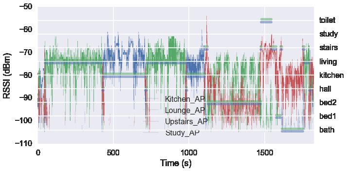
kitchen, living room, master bedroom, and the study. The RSSI signals that were recorded by the
four access points are shown in 3b, and the localisation labels are also overliad on this image
(c.f. to Figure 2).
This image shows that there is a close relationship between the values of RSSI and location.
Taking a concrete example, we can see that during the first 500 seconds, a significant proportion
of time is spent in the living room. The access point in the living room (i.e. the green trace)
reports the highest response, and the remaining access points have not registered the connection.
6//
(a) Acceleration signal trace shown over a 5 minute time period. Annotations are
overlaid in blue and green.
(b) RSSI values from the four access points. Room occupancy labels are shown by
the the horizontal lines.
Figure 3: Example acceleration and RSSI signals for training record 00001. The line traces indi-
cate the accelerometer/RSSI values recorded by the access points. The horizontal lines indicate
the ground-truth as provided by the annotators (two annotators annotated this record, and their
annotations are depicted by the green and blue traces respectively.
7Consequently, the RSSI and the PIR are both valuable signals for localisation.
It is worth noting that the Bluetooth link is set up in ‘connectionless’ mode. This mode in-
creases the live cycle of the wearable battery, and also allows the wearable data to be acquired
simultaneously by multiple access points. However, the data are also transmitted with a lower
Quality of Service (QoS) which increases the risk of lost packets. This is particularly clear in 3b
since at no time is data received on all access points. Similarly, in 3a acceleration packets are lost.
3.1.3. Video data
Video recordings were taken using ASUS Xtion PRO RGB-Depth (RGBD) cameras1 . Auto-
matic detection of humans was performed using the OpenNI library2 . False positive detections
were manually removed by the organisers by visual inspection. Three RGBD cameras are in-
stalled in the SPHERE house, and these are located in the living room, downstairs hallway, and
the kitchen. No cameras are located elsewhere in the residence.
In order to preserve the anonymity of the participants the raw video data are not available,
and instead the coordinates of the 2D bounding box, 2D centre of mass, 3D bounding box and
3D centre of mass are provided. The units of 2D coordinates are in pixels (i.e. number of pixels
down and right from the upper left hand corner) from an image of size 640 × 480 pixels. The
coordinate system of the 3D data is axis aligned with the 2D bounding box, with a supplementary
dimension that projects from the central position of the video frames. The first two dimensions
specify the vertical and horizontal displacement of a point from the central vector (in millimetres),
and the final dimension specifies the projection of the object along the central vector (again, in
millimetres).
Examples of the centre of the 3D bounding box are shown in Figure 4 where the three video
locations are separated according to their location. Video data is rich in the information that it pro-
vides, and it is informative for predicting location and ADLs. Room-level location can be inferred
since each camera is situated in a room. Additionally, with appropriate feature engineering, it is
possible to determine activities of daily living. However, since cameras are only available in three
rooms, we cannot rely purely on RGBD features for localisation or ADL.
3.2. Recruitment and Sensor Layout
Twenty participants were recruited to perform activities of daily living in the SPHERE house
while the data recorded by the sensors was logged to a database. Ethical approval was secured
from the University of Bristol’s ethics committee to conduct data collection, and informed consent
was obtained from healthy volunteers.
In the first stage of data collection, participants were requested to follow a pre-defined script.
1a 1b and 1c show the floor plan of the ground, first and second floors of the smart environment
respectively.
1
https://www.asus.com/3D-Sensor/Xtion_PRO/
2
https://github.com/OpenNI/OpenNI
8Figure 4: Example centre 3d for training record 00001. The horizontal lines indicate annotated
room occupancy. The blue, green and red traces are the x, y, and z values for the 3D centre of
mass.
3.3. Annotation
A team of 12 annotators were recruited and trained to annotate the locations of ADLs. To
support the annotation process, a head mounted camera (Panasonic HX-A500E-K 4K Wearable
Action Camera Camcorder) recorded 4K video at 25 FPS to an SD-card. This data is not shared in
this dataset, and is used only to assist the annotators. Synchronisation between the network time
protocol (NTP) clock and the head-mounted camera was achieved by focusing the camera on an
NTP-synchronised digital clock at the beginning and end of the recording sequences.
An annotation tool called ELAN3 was used for annotation. ELAN is a tool for the creation
of complex annotations on video and audio resources, developed by the Max Planck Institute for
Psycholinguistics in Nijmegen, The Netherlands.
Room occupancy labels are also given in the training sequences. While performance evaluation
is not directly affected by room prediction on this, participants may find that modelling room
occupancy may be informative for prediction of posture and ambulation.
3.4. Performance evaluation
As both the targets and predictions are probabilistic, the standard classification performance
evaluation metrics are inappropriate. Hence, classification performance is evaluated with weighted
3
https://tla.mpi.nl/tools/tla-tools/elan/
9Brier score [4]:
N C
1 XX
BS = wc (pn,c − yn,c )2 (1)
N n=1 c=1
where N is the number of test sequences, C is the number of classes, wc is the weight for each
class, pn,c is the predicted probability of instance n being from class c, and yn,c is the proportion
of annotators that labelled instance n as arising from class c. Lower Brier score values indicate
better performance, with optimal performance achieved with a Brier score of 0.
4. Bayesian Sensor Fusion
In this section we will develop a class of models that may be used to tackle the two sensor
fusion tasks described above. Critically, we will also show how these two can be combined into a
single model.
4.1. Preliminaries
We will begin by assuming that distributions (or densities) over a set of variables x = (x1 , . . . xD )
of interest can be represented as factor graphs, i.e.
J
1Y
p(x) = ψj (xne(ψj ) ), (2)
Z j=1
where ψj are the factors: non-negative functions defined over subsets of the variables xne(ψj ) ,
the neighbours of the factor node ψj in the graph, where we use ne(ψj ) to denote the set indices
of the variables of factor ψj ). Z is the normalisation constant. We only consider here directed
factors ψ(xout |xin ) which specify a conditional distribution over variables xout given xin (hence
xne(ψ) = (xout , xin )). For more details see e.g. [14, 3].
4.2. Multi-Class Bayes Point Machine
We begin by describing a Bayesian model for classification known as the multi-class Bayes
Point Machine (BPM) [12], which will form the basis of our modelling approach. The BPM
makes the following assumptions:
1. The feature values x are always fully observed.
2. The order of instances does not matter.
3. The predictive distribution is a linear discriminant of the form p(yi |xi , w) = p(yi |si = w0 xi )
where w are the weights and si is the score for instance i.
4. The scores are subject to additive Gaussian noise.
5. The features are as uncorrelated as possible. This allows modelling p(w) as fully factorised
6. (optional) A factorised heavy-tailed prior distributions over the weights w
10For the purposes of both location prediction and activity recognition, assumption 2 may be
problematic, since the data is clearly sequential in nature. Intuitively, we might imagine that the
strength of the temporal dependence in the sequence will determine how costly this approximation
is, and this will in turn depend on how the data is preprocessed (i.e. is raw data presented to
the classifier, or are features instead computed from the time series?). It has been shown [21] that
under certain conditions structured models and unstructured models can yield equivalent predictive
performance on sequential tasks, whilst unstructured models are also typically much cheaper to
compute. We follow the guidance set out there and use contextual information from neighbouring
time-points to construct our features.
The factor graph for the basic multi-class BPM model is illustrated in 5a, where N denotes a
Gaussian density for a given mean µ and precision τ , and Γ denotes a Gamma density for given
shape k and scale θ. The factor indicated by is the arg-max factor, which is like a probabilistic
multi-class switch. The additive Gaussian noise from assumption 4 results in the variable s̃, which
is a noisy version of the score s.
An alternative to the arg-max factor is the softmax function, or normalised exponential
function, which is a generalisation of the logistic function that transforms a K-dimensional vector
z of arbitrary real values to a K-dimensional vector σ(z) of real values in the range (0, 1) that sum
to 1. The function is given by
e zj
σ(zj ) = PK j = 1, . . . , K.
k=1 e zk
Multi-class regression involves constructing a separate linear regression for each class, the output
of which is known as an auxiliary variable. The vector of auxiliary variables for all classes is put
through the softmax function to give a probability vector, corresponding to the probability of
being in each class.
Multi-class softmax regression is very similar in spirit to the multi-class BPM. The key
differences are that where the BPM uses a max operation constructed from multiple “greater than”
factors, softmax regression uses the softmax factor, and Variational Message Passing (VMP)
(see subsection 5.1) is currently the only option when using the softmax factor. Two conse-
quences of these differences are that softmax regression scales computationally much better
with the number of classes than the BPM (linear rather quadratic complexity) and although not
relevant here it is possible to have multiple counts for a single sample (multinomial regression).
In this case the number of classes C is not so large, meaning that the quadratic O(C 2 ) scaling of
the BPM is not so problematic.
We also propose to use a heavy-tailed prior, a Gaussian distribution whose precision is itself a
mixture of Gamma-Gamma distributions. This is illustrated in the factor graph in 5b, where N
denotes a Gaussian density for a given mean µ and precision τ , and Γ denotes a Gamma density
for given shape and rate). The variable a is a common precision that is shared by all features, and
the variable b represents the precision rate, which adapts to the scaling of the features. Compared
with a Gaussian prior, the heavy-tailed prior is more robust towards outliers, i.e. feature values
which are far from the mean of the weight distribution, 0. It is invariant to rescaling the feature
values, but not invariant to their shifting, which is achieved by adding a constant feature value
11(bias) for all instances.
(1, 1)
1
(1, 1) r
0 1
N a / b
0
w x 0 τ N
N
×
D w x
s 1 ×
D
N 1 w x
s
D
N BPM
s̃
C s̃ s̃
C C
y y y
N N N
(a) (b) (c)
Figure 5: (a) Multi-class Bayes Point Machine; (b) heavy-tailed version; and (c) simplified repre-
sentation. C: Number of classes; N : Number of examples; D: Number of features. See text for
details.
In 5c we also give a simplified form of the factor graph, where the essential parts of the BPM
have been collapsed into a single bpm factor. We will use the simplified form in further models to
aid the presentation, but should be born in mind that this actually represents 5a or 5b depending
on the context.
In this form, the model is not identifiable, since the addition of a constant value to all the
score variables s will not change the output of the prediction. To make the model identifiable we
enforce that the score variable corresponding to the last class will be zero, by constraining the last
coefficient vector and mean to be zero.
4.3. Fused Bayes Point Machine
The simplest method for fusing multiple sensing modalities is to concatenate all of the features
from each modality for each example into a single long feature vector. This can then be presented
12to the BPM as described above, and will serve as a baseline model.
Here we present three Bayesian models for sensor fusion. the first of these, shown in 6a, is the
simplest of these, and corresponds quite closesly to the unweighted probabilistic MKL model
given in [5]. Taking the simplified factor graph in 5c, we have an additional plate over the
sources/modalities S, for the entire BPM model, which results in a noisy score s̃ for each source.
These are then summed together to get a fused score per class, and the standard arg-max or
softmax link function can then be used.
The first modification of this is the weighted additive fusion model shown in 6b. Here we
have additional variables β per source, which are than multiplied with the noisy scores before
addition to give fused scores. This model provides extra interpretability since the means of the
β variables indicate the influence of the source associated with that variable, and the variances
of these variables indicate the overall uncertainty about that source. However this model also
introduces extra symmetries that can cause difficulties in inference.
The second modification is the switching model presented in 6c. In this model, we have a
single switching variable z which follows a categorical distribution that is defined over the range
of the sources. This categorical distribution is parametrised by the probability vector θ, which
follows a uniform Dirichlet distribution.
w x
D
BPM
(0, 1) Dir
w x β s̃ w x
D C D
×
BPM
θ BPM
f
Cat
s̃ s̃
S
C
+ + z Switch
S
f t t
S C
y y y
N N N
(a) (b) (c)
Figure 6: Bayesian multi-class fusion classification models: (a) unweighted additive version; (b)
weighted additive version; and (c) fused switching model. S: Number of sources. See text for
details.
134.4. Stacked classifiers
The models described thus far have all been designed to tackle fusion of multiple sources to
achieve a single multi-class classification task. However, in the SPHERE challenge setting, there
are in fact two classification tasks: firstly, there is the classification of location, based on the
fusion of RSSI values from the wearable device along with the stationary PIR sensors. Secondly,
there is the classification of the activity being performed, based on the fusion of the wearable
accelerometer readings and the video bounding boxes. It is a reasonable hypothesis that certain
activities are much more likely to occur in some locations than others: hence, we propose another
form of fusion, to train activity recognition models for each location use the location prediction
model to switch over these models.
This could of course be done in a two stage process, where the switch could take the a weighted
combination of the predictions from the location predictions to produce a fused prediction (again
this can form a strong baseline). However we also surmise that there may be an advantage to
be gained by learning both stages in a single model, since the activity recognition models could
inform the location prediction as well. This model is depicted in Figure 7. Note that the location
predictions yL now act as a probabilistic switching variable over the activity BPMs, of which there
is one per location. For simplicity, we have omitted the fusion parts of this model, but note that
we can incorporate any of the 3 kinds of fusion found in Figure 6.
w x
DL
BPM
s̃
L
yL
wA xA
DA
BPM
s̃A
A
yA
N
Figure 7: Stacked classification model for simultaneous location prediction and activity recogni-
tion. L: Number of locations; A: Number of activities N : Number of examples; DL : Number of
location features. DA : Number of activity features. See text for details.
145. Methodology
5.1. Inference
The Belief Propagation (BP) (or sum-product) algorithm computes marginal distributions over
subsets of variables by iteratively passing messages between variables and factors within a given
graphical model, ensuring consistency of the obtained marginals at convergence. Unfortunately,
for all but trivial models, exact inference using BP is intractable. In this work, we employ two
separate inference algorithms, both of which are efficient deterministic approximations based on
message-passing over the factor graphs we have seen before.
Expectation Propagation (EP) [17] introduces an approximation in the case when the messages
from factors to variables do not have a simple parametric form, by projecting the exact marginal
onto a member of some class of known parametric distributions, typically in the exponential fam-
ily, e.g. the set of Gaussian or Beta distributions.
VMP applies variational inference to Bayesian graphical models [24]. VMP proceeds by send-
ing messages between nodes in the network and updating posterior beliefs using local operations
at each node. Each such update increases a lower bound on the log evidence at that node, (unless
already at a local maximum). VMP can be applied to a very general class of conjugate-exponential
models because it uses a factorised variational approximation, and by introducing additional vari-
ational parameters, VMP can be applied to models containing non-conjugate distributions.
EP and VMP has a major advantage over sampling methods in this setting, which is that it is
relatively easy to compute model evidence (see Equation (??) in below). In the case of VMP, this
is directly available from the lower bound. The evidence computations can be used both for model
comparison and for detection of convergence.
5.2. Model Comparison
We would also like perform Bayesian model comparison, in which we marginalise over the
parameters for the type of model being used, with the remaining variable being the identity of
the model itself. The resulting marginalised likelihood, known as the model evidence, is the
probability of the data given the model type, not assuming any particular model parameters. Using
D for data, θ to denote model parameters, H as the hypothesis, the marginal likelihood for the
model H is
Z
p(D|H) = p(D|θ, H) p(θ|H) dθ (3)
This quantity can then be used to compute the Bayes factor [11], which is the posterior odds ratio
for a model H1 against another model H2 ,
p(H1 |D) p(H1 )p(D|H1 )
= . (4)
p(H2 |D) p(H2 )p(D|H2 )
5.3. Batch and Online Learning
There may be occasions when the full model will not fit in memory at once (either at train time
or prediction time), as is the case for the SPHERE challenge dataset when performing inference
15on a standard desktop computer. In this case, there are two options: batched inference and online
learning. Infer.NET provides a SharedVariable class, supports sharing between models of different
structures and also across multiple data batches, and makes it easy to implement batched inference.
Online learning is performed using the standard assumed-density filtering method of [18], which
in the case of the weight variables which are marginally Gaussian distributed, simply equates to
setting the priors to be the poteriors from the previous round of inference.
5.4. Data pre-processing
We further perform standardisation (whitening) for each feature within each source indepen-
dently. Whilst this is not strictly necessary for the heavy-tailed models, it will not negatively
impact on their performance so is done for all models to ensure consistency. We further add a
constant bias feature (equal to 1) per source.
We also augment the feature space by adding polynomial degree 2 interaction features for each
source, meaning that we in effect performing polynomial regression. This is equivalent to the
implicit feature space of a degree 2 polynomial kernel in kernel methods, which intuitively, means
that both features and pairwise combinations of features are taken into account. When the input
features are binary-valued, then the features correspond to logical conjunctions of input features.
Note that this method roughly doubles the number of variables in the model, but in this case the
feature spaces are of relatively low dimension.
6. Discussion
Prediction performance is the one clear motivation for the use of models for fusion. However,
even if prediction performance is not improved (or degraded in non-significant ways) it can provide
other benefits. These include extra interpretability of the models by looking at how the modalities
are used by the models, and potentially robustness to missing modalities, since the models can be
encouraged to use all of the modalities even when they provide less information for predictions.
It might be possible to achieve such robustness with a simple BPM through re-weighting features
on the basis of the posteriors from training, but it would clearly be more satisfying if this could
achieved only by changing mixing coefficients to get the same effect.
6.1. Early versus late fusion
Generally speaking, the literature describes early and late fusion strategies [20]. Early fusion
is a usually described as a scheme that integrates unimodal features before learning concepts.
This would include strategies such as concatenating feature spaces and (probabilistic) MKL [1, 5].
Late fusion is a scheme that first reduces unimodal features to separately inferred concept scores
(e.g. through independent classifiers), after which these scores are integrated to learn concepts,
typically using a further classification algorithm. [20] showed empirically that late fusion tended
to give slightly better performance for most concepts, but for those concepts where early fusion
performs better the difference was more significant.
The methods described in this paper fit more in line with the late fusion scheme under this
definition, since the fusion is occurring at the score level. However the framework laid out here is
more principled, since there is no recourse to two sets of classification algorithms and the heuristic
manipulations that they entail.
166.2. Transfer Learning
As shown in [10], it is possible to extend the multi-class BPM [12] to the transfer learning
setting by adding an additional layer of hierarchy to the model. To deal with the transfer of
learning between individuals (residents), we would have an extra plate around the individuals that
are present in the training set (R), who form the community, allowing us to learning shared weights
for the community.
To apply our learnt community weight posteriors to a new individual we can use the same
model configured for a single individual with the priors over weight mean and weight precision
replaced by the Gaussian and Gamma posteriors learnt from the individuals in the training set
respectively. This model is able to make predictions even when we have not seen any data for
the new individual, but it is also possible to do online training as we receive labelled data for the
individual. By doing so, we can smoothly evolve from making generic predictions that may apply
to any individual to making personalised predictions specific to the new individual. Note that as
stated this only applies to the version of the model without heavy-tailed priors, but can be extended
to this setting as well.
Note that it is also possible to separate the community priors into groups (e.g. by demographics
or medical condition) by having hyper-priors for each group, a separate indicator variable indicat-
ing group membership, acting as a gating variable to select the appropriate hyper-priors.
The separate transfer learning problem from house-to-house is achieved through the method
of introducing meta-features of [19], and then the feature space is automatically mapped from the
source domain to the target domain. In order to apply this to the models discussed in section 4,
we would assume that the features x have already been mapped to these meta-features, and that
similarly for the personalisation phase the mapping has already taken place.
7. Conclusions
There is a widely-accepted need to revise current forms of health-care provision, with par-
ticular interest in sensing systems in the home. Given a multiple-modality sensor platform with
heterogeneous network connectivity, as is under development in the Sensor Platform for HEalth-
care in Residential Environment (SPHERE) Interdisciplinary Research Collaboration (IRC), we
face specific challenges relating to the fusion of the heterogeneous sensor modalities. We further
will require the transfer of learnt models to a deployment context that may differ from the training
context.
We introduce Bayesian models for sensor fusion, which aim to address the challenges of fusion
of heterogeneous sensor modalities.Using this approach we are able to identify the modalities that
have most utility for each particular activity, and simultaneously identify which features within
that activity are most relevant for a given activity.
We further show how the two separate tasks of location prediction and activity recognition can
be fused into a single model, which allows for simultaneous learning an prediction for both tasks.
We analyse the performance of this model on data collected in the SPHERE house, and show
its utility. We also compare against some benchmark models which do not have the full structure,
and show how the proposed model compares favourably to these methods.
17Acknowledgements
This work was performed under the SPHERE IRC funded by the UK Engineering and Physical
Sciences Research Council (EPSRC), Grant EP/K031910/1. The project is actively working to-
wards releasing high-quality data sets to encourage community participation in tackling the issues
outlined here.
References
[1] Bach, F. R., Lanckriet, G. R., Jordan, M. I., 2004. Multiple kernel learning, conic duality, and the smo algorithm.
In: Proceedings of the twenty-first international conference on Machine learning. ACM, p. 6.
[2] Bishop, C., 2013. Model-based machine learning. Phil Trans R Soc A 371.
[3] Bishop, C. M., et al., 2006. Pattern recognition and machine learning. Vol. 4. springer New York.
[4] Brier, G. W., 1950. Verification of forecasts expressed in terms of probability. Monthly weather review 78 (1),
1–3.
[5] Damoulas, T., Girolami, M. A., 2008. Probabilistic multi-class multi-kernel learning: on protein fold recognition
and remote homology detection. Bioinformatics 24 (10), 1264–1270.
[6] Diethe, T., Girolami, M., 2013. Online learning with (multiple) kernels: A review. Neural Computation 25,
567–625.
[7] Diethe, T., Hardoon, D. R., Shawe-Taylor, J., 2008. Multiview Fisher discriminant analysis. In: NIPS 2008
workshop “Learning from Multiple Sources”.
[8] Diethe, T., Hardoon, D. R., Shawe-Taylor, J., 2010. Constructing nonlinear discriminants from multiple data
views. In: ECML/PKDD. Vol. 1. pp. 328–343.
[9] Diethe, T., Twomey, N., Flach, P., 2014. SPHERE: A sensor platform for healthcare in a residential environment.
In: Proceedings of Large-scale Online Learning and Decision Making Workshop.
[10] Diethe, T., Twomey, N., Flach, P., 2016. Active transfer learning for activity recognition. In: European Sympo-
sium on Artificial Neural Networks, Computational Intelligence and Machine Learning.
[11] Goodman, S. N., 1999. Toward evidence-based medical statistics. 2: The Bayes factor. Annals of internal
medicine 130 (12), 1005–1013.
[12] Herbrich, R., Graepel, T., Campbell, C., January 2001. Bayes point machines. Journal of Machine Learning
Research 1, 245–279.
[13] Klein, L. A., 2004. Sensor and data fusion: a tool for information assessment and decision making. Vol. 324.
Spie Press Bellingham, WA.
[14] Kschischang, F. R., Frey, B. J., Loeliger, H.-A., 2001. Factor graphs and the sum-product algorithm. IEEE
Transactions on information theory 47 (2), 498–519.
[15] Liu, H., Motoda, H., 1998. Feature extraction, construction and selection: A data mining perspective. Springer.
[16] May, B. C., Korda, N., Lee, A., Leslie, D. S., Jun. 2012. Optimistic bayesian sampling in contextual-bandit
problems. J. Mach. Learn. Res. 13, 2069–2106.
[17] Minka, T. P., 2001. Expectation propagation for approximate Bayesian inference. In: Proceedings of the Seven-
teenth conference on Uncertainty in artificial intelligence. Morgan Kaufmann Publishers Inc., pp. 362–369.
[18] Opper, M., 1998. A Bayesian approach to on-line learning. In: Saad, D. (Ed.), On-line Learning in Neural
Networks. Cambridge University Press, New York, NY, USA, pp. 363–378.
[19] Rashidi, P., Cook, D. J., Jun. 2011. Activity knowledge transfer in smart environments. Pervasive Mob. Comput.
7 (3), 331–343.
[20] Snoek, C. G., Worring, M., Smeulders, A. W., 2005. Early versus late fusion in semantic video analysis. In:
Proceedings of the 13th annual ACM international conference on Multimedia. ACM, pp. 399–402.
[21] Twomey, N., Diethe, T., Flach, P., 2016. On the need for structure modelling in sequence prediction. Machine
Learning 104 (2), 291–314.
URL http://dx.doi.org/10.1007/s10994-016-5571-y
[22] Twomey, N., Diethe, T., Kull, M., Song, H., Camplani, M., Hannuna, S., Fafoutis, X., Zhu, N., Woznowski, P.,
18Flach, P., Craddock, I., 2016. The SPHERE challenge: Activity recognition with multimodal sensor data. arXiv
preprint arXiv:1603.00797.
[23] Winn, J., Bishop, C. M., Diethe, T., 2015. Model-Based Machine Learning. Microsoft Research Cambridge.
URL http://www.mbmlbook.com
[24] Winn, J. M., Bishop, C. M., 2005. Variational message passing. In: Journal of Machine Learning Research. pp.
661–694.
[25] Woznowski, P., Burrows, A., Camplani, M., Diethe, T., Fafoutis, X., Hall, J., Hannuna, S., Kozlowski, M.,
Twomey, N., Tan, B., Zhu, N., Elsts, A., Vafeas, A., Mirmehdi, M., Burghardt, T., Damen, D., Paiement, A., Tao,
L., Flach, P., Oikonomou, G., Piechocki, R., Craddock., I., 2016. SPHERE: A Sensor Platform for HEalthcare
in a Residential Environment. In: Angelakis, V., Tragos, E., Pöhls, H., Kapovits, A., Bassi, A. (Eds.), Designing
and Developing and and Facilitating Smart Cities: Urban Design to IoT Solutions. Springer.
[26] Woznowski, P., Fafoutis, X., Song, T., Hannuna, S., Camplani, M., Tao, L., Paiement, A., Mellios, E., Haghighi,
M., Zhu, N., et al., 2015. A multi-modal sensor infrastructure for healthcare in a residential environment. In:
Communication Workshop (ICCW), 2015 IEEE International Conference on. IEEE, pp. 271–277.
[27] Zhu, N., Diethe, T., Camplani, M., Tao, L., Burrows, A., Twomey, N., Kaleshi, D., Mirmehdi, M., Flach, P.,
Craddock, I., 2015. Bridging e-health and the internet of things: The SPHERE project. Intelligent Systems,
IEEE 30 (4), 39–46.
19You can also read