Hypothesis-driven Stream Learning with Augmented Memory - Kreiman Lab

Hypothesis-driven Stream Learning with Augmented Memory

 Mengmi Zhang1,2,* , Rohil Badkundri1,2,3,* , Morgan B. Talbot2,4 , and Gabriel Kreiman1,2

 *
 Equal contribution
 Address correspondence to gabriel.kreiman@tch.harvard.edu
 1
 Children’s Hospital, Harvard Medical School
arXiv:2104.02206v2 [cs.CV] 7 Apr 2021

 2
 Center for Brains, Minds and Machines
 3
 Harvard University
 4
 Harvard-MIT Health Sciences and Technology, Harvard Medical School

 Figure 1: Schematics of two stream learning protocols in the incremental class settings: learning with class iid data (a)
 and class instance data (b). In the incremental class setting, for each task, the model has to learn to classify 2 new classes
 while training for a single epoch. During testing, the model has to classify images from all seen classes without knowing task
 identity. In incremental class iid, within a task, the sequence of images is randomly shuffled, whereas in class instance, the
 temporal order of images is preserved. See Sec 3.1 for protocol descriptions.

 Abstract on three stream learning object recognition datasets. Our
 method performs comparably well or better than SOTA
 methods, while offering more efficient memory usage. All
 Stream learning refers to the ability to acquire and source code and data are publicly available https://
 transfer knowledge across a continuous stream of data github.com/kreimanlab/AugMem.
 without forgetting and without repeated passes over the 1. Introduction
 data. A common way to avoid catastrophic forgetting is
 to intersperse new examples with replays of old examples Stream learning enables continual acquisition and
 stored as image pixels or reproduced by generative transfer of new knowledge from a temporally structured
 models. Here, we considered stream learning in image input sequence while retaining previously learnt
 classification tasks and proposed a novel hypotheses-driven experiences [10]. This ability is critical for artificial
 Augmented Memory Network, which efficiently consolidates intelligence (AI) systems to interact with the world and
 previous knowledge with a limited number of hypotheses process continuous streams of information [32]. Stream
 in the augmented memory and replays relevant hypotheses learning remains a long-standing challenge for neural
 to avoid catastrophic forgetting. The advantages of networks that typically learn representations offline from
 hypothesis-driven replay over image pixel replay and stationary training batches [24, 27, 7]. When faced with
 generative replay are two-fold. First, hypothesis-based streams where data are not independent and identically
 knowledge consolidation avoids redundant information in distributed (iid), and where data are provided continuously
 the image pixel space and makes memory usage more without access to old data, SOTA AI systems tend to fail
 efficient. Second, hypotheses in the augmented memory can to retain good performance across previously learnt tasks
 be re-used for learning new tasks, improving generalization [11, 16, 23]. Numerous methods for alleviating catastrophic
 and transfer learning ability. We evaluated our method forgetting have been proposed, the simplest being to jointly

train models on both old and new tasks, which demands a In replay methods, a subset of images or features
large amount of resources to store previous training data from a previous task are stored or generated and later
and hinders learning of novel data in real time. shown to the model to prevent forgetting. Compared with
 Inspired by memory-augmented networks in few-shot weight regularization, replay methods lead to enhanced
image classification [30], memory retrieval tasks [8], performance [28, 25]. Raw-pixel replay, where subsets
and video prediction [9], we proposed an augmented of images from previous tasks are stored and later
memory architecture, Hypothesis-driven Augmented replayed, involves highly redundant information and is
Memory Network (HAMN), for stream learning in memory-inefficient. Moreover, relying on limited sets
image classification tasks. The network learns a set of replay images can lead to overfitting. In contrast,
of hypotheses in the augmented memory, such that the our method better generalizes by learning discriminative,
latent representation of an image can be constructed information-rich hypotheses in latent space, which can then
by a linear combination of the hypotheses. Multi-head be re-used to construct multiple new samples in the latent
content-based attention allows the model to share the space for replay and to transfer knowledge to new tasks.
augmented memory over multiple image features, further To avoid having to store many images, generative replay
compressing representations in memory and allowing systems complement each new task with ”pseudo-data” that
features to be reconstructed from hypotheses in parallel. resembles historical data and is produced by a generative
 To prevent catastrophic forgetting, we imposed three model. [31, 29]. In particular, Deep Generative Replay
constraints on HAMN. First, to preserve encoded (DGR) [31] is a Generative Adversarial Network that
hypotheses in augmented memory, we regularized the synthesizes training data over all previously learnt tasks.
network to write new hypotheses into rarely-used locations Generative approaches have succeeded with simple and
in memory. Second, we stored the memory indices artificial datasets but cannot tackle more complicated inputs
activated by samples from previous tasks, reconstructed [2]. Moreover, to synthesize historical data reasonably
these samples from the corresponding hypotheses, and well, the size of the generative model tends to be large and
replayed the constructed samples during training. Finally, expensive with respect to memory resources [35].
we applied logit matching [28] during replay to maintain
 Finally, previous work [11] has suggested that instead
the learnt class distributions from all previous tasks.
 of replay with raw pixels, replay of latent image features
 We evaluated our method under two typical stream
 using memory indexing is more efficient and effective at
learning protocols (Figure 1), incremental class iid
 preventing catastrophic forgetting. However, this method
and incremental class instance, across three benchmark
 relies on Product Quantization [15], where a codebook for
datasets, CORe50 [21], Toybox [34] and iLab [3]. The
 constructing the memory is pre-computed and fixed. This
performance of HAMN is comparable to or even better than
 hinders the ability of the model to learn and adapt to new
state-of-the-art (SOTA) methods. HAMN demonstrates the
 tasks. In this work, as opposed to fixed codebooks, our
capabilities of memory retention and adaptation to new
 proposed method learns a set of discrete hypotheses on the
tasks, even while going through a continuous stream of
 fly and replays constructed samples from the set of learnt
training examples only once.
 hypotheses based on a memory indexing mechanism learnt
 throughout new tasks.
2. Related Works
 Stream learning approaches can be categorized into
(1) weight regularization and (2) replay methods. Weight 3. Stream Learning Protocols and Datasets
regularization stores the weights of the model trained
on previous tasks and imposes constraints on weight 3.1. Stream Learning Protocols
updates for new tasks [12, 17, 37, 19, 22]. For example,
 Both stream learning protocols are variations of the
Learning Without Forgetting (LwF) [20] stores all the
 incremental class setting (Figure 1), defined below:
model parameters on previously learnt tasks, estimates
their importance on previous tasks, and penalizes future Class-iid: Within each task, all of the images from two
changes to these parameters on new tasks. However, classes are randomly shuffled. Each image in the task is
selecting the “important” parameters for previous tasks seen by the model once.
via pre-defined thresholds complicates the implementation Class-instance: Each task contains a series of
by necessitating exhaustive hyper-parameter tuning. temporally-ordered images from the object instances
In addition, state-of-the-art recognition models often corresponding to the chosen classes. An object instance
involve millions of parameters, and therefore storing the refers to a series of images of a particular object taken
“importance” values for each network parameter across all under specific conditions, such as a background or a spatial
previous tasks can be costly [35]. transformation. The model is trained for one epoch.

3.2. Datasets soft class distribution predicted from the constructed and
 the extracted feature maps, respectively.
The CORe50 dataset [21] contains sequences of video
frames for a collection of 50 objects organized into 10 4.2. Feature Extraction and Classification
classes. Object instances are 15 second video clips of
an object under particular conditions and poses, with 11 The 2D-CNN contains two nested functions: F (·) for
instances per object. We follow the work [11] to come up feature extraction, parameterized by θF , consisting of the
with the ordering, training and testing data splits. first few convolution blocks; and Pt (·) for classification,
The Toybox dataset [34] contains videos of toy objects parameterized by θPt at task t, consisting of the last few
from 12 classes. We used a subset of the full dataset convolution blocks. Since the first few convolution layers in
containing 348 toy objects with 10 instances per object, 2D-CNN are highly transferable [36], the feature extractor
each containing a spatial transformation of that object’s F (·) keeps parameters θF fixed over all tasks. θF is trained
pose. We sampled each instance at 1 frame per second for object recognition using ImageNet [6]. The parameters
resulting in 15 images per transformation per object. We θPt in Pt (·) depend on task t. After pre-training on
chose 3 of the 10 transformations for our test set, leaving ImageNet, we fine-tune Pt (·) such that HAMN learns new
the remaining instances for training. sets of hypotheses and decision boundaries incrementally to
The iLab dataset [3] contains images of toy vehicles. classify new object classes.
We used a subset of the full dataset containing 392 Up to task t, HAMN has seen a total of Ct classes. Given
vehicle objects from 14 classes, with 8 distinct backgrounds an image It shown during task t, we define the output tensor
(instances) per object and 15 images per instance. We chose Zt from the feature extraction step as Zt = F (It ). Zt
2 of the 8 instances per object for our test set, leaving the is of size S × W × H for channels, width, and height
remaining instances for training. respectively. The output feature maps Zt can then be used
 to produce a logits vector qt = Pt (Zt ). The logits vector
4. Our proposed method (HAMN) qt ∈ RCt contains the activation values over all Ct seen
 classes and is then passed as input to the softmax function,
4.1. Overview which outputs the predicted probability vector pt ∈ RCt
 over all Ct classes.
The HAMN model consists of a 2D convolutional neural
 We used pt (c) and qt (c) to denote the predicted
network (2D-CNN) coupled with an augmented memory
 probability and logit value for class c respectively. We
bank represented as a 2D matrix (Figure 2). The memory
 define Lclassi (·) as the cross-entropy loss between pt and
matrix stores a fixed number of hypotheses, with a single
 its corresponding ground truth class label yc :
hypothesis per memory slot. In image classification, Ct
 X
HAMN first takes an image as input and extracts its Lclassi (pt , yc ) = − δ(i = yc ) log(pt (i)) (1)
feature maps at an intermediate layer of the 2D-CNN. i=1
By computing the similarity between the extracted feature
maps and the stored hypotheses, the reading attention where δ(x) = 1 if x = yc and δ(x) = 0 otherwise.
mechanism guides the reading heads to select a linear
 4.3. Augmented Memory
combination of hypotheses, with higher attention weights
assigned to memory slots with content more similar to We define Mt as the contents of the memory bank of
the feature maps. To further compress the hypotheses in size N × M at task t. There are N memory slots,
augmented memory while maintaining rich representations, with each memory slot storing a hypothesis vector of
we use a multi-head reading attention to interact with dimension M . We use index i to denote the ith
the memory bank. This is achieved by splitting the memory slot (i ∈ {1, 2, ..., N }). Thus, we have Mt =
feature maps into segments, with each segment interacting [Mt (1), Mt (2), ..., Mt (i), ..., Mt (N )] where Mt (i) is a
with the same memory bank using its individual reading hypothesis vector indexed by i.
attention head. The number of plausible feature maps Multi-head content-based reading attention
that can be constructed increases exponentially with the The feature extractor F (·) serves as a controller and
number of reading heads and hypotheses, enabling a diverse outputs the tensor Zt as the reading key of image It .
representation space. Based on the content similarity between Zt and each
 The latter part of the 2D-CNN combines the constructed hypothesis in the memory bank Mt , a content-based
feature maps with the hypotheses in the memory bank memory addressing mechanism is used to draw a hypothesis
for classification. To ensure the memory bank learns from Mt . Ideally, one could store the individual Zt of each
useful hypotheses for replay in later tasks, in addition to image It as a hypothesis in the memory bank and replay
a classification loss, we imposed an additional logistic loss, each hypothesis to prevent catastrophic forgetting, but this
commonly used in knowledge distillation [13], based on the requires extensive memory resources. To further compress

Augmented memory (N × ) in Task = 
 Classify new images softmax
 in Task = Hypothesis vector 1 × 
 Multi-head … 1

 Position Index
 Content-based 2
 Reading 3
 Attention

 …
 …

 …

 …
 …
 … 
 Feature extractor
 (pre-trained … Classification Net
 …
 and fixed weights)
 ∗ shared
 Predicted labels
 “glasses”
 Hypothesis-driven weights
 
 Reconstruction
 Classification Net
 Memory Replay Convert Memory Indices Augmented memory (N × ) in Task = 
 for Task = 1, 2, …, − To attention vectors Hypothesis vector 1 × 
 … 1

 Position Index
 Stored Memory Stored logits 2 Stored logits
 Indices
 3
 …
 …

 …
 …

 …
 …
 Replay each
 … 
 stored pair 
 
 …
 Predicted labels
 Classification Net
 …
 …

 ∗ … “scissors”
 …

 Least used memory loss 
 … 
 
 Hypothesis-driven
 Reconstruction

Figure 2: Schematic illustration of the proposed hypotheses-driven Augmented Memory Network (HAMN) for stream
learning tasks. HAMN model consists of a 2D-CNN and an augmented memory containing a set of hypotheses. The
feature extractor in the 2D-CNN acts as a controller and decides which hypotheses to retrieve from the memory based on a
content-similarity addressing mechanism. To further compress the memory and increase representation variety, multi-head
reading attention is used. The re-constructed feature maps from the augmented memory (dashed line box) can be used for
classification loss Lnew
 classi . To ensure these hypothesis-driven feature maps are as discriminative as the output of the CNN
feature extractor, a logit distillation loss Lnewdistill is used between the two. To avoid catastrophic forgetting, we stored the
memory indices of retrieved hypothesis along with the corresponding logits from previous tasks. During replay (shaded
area), we used the stored memory indices to re-construct feature maps for classification loss Lold classi and stored logits
for regularization based on Lold distill . Least used memory loss Lmem is imposed to prevent HAMN from over-writing the
frequently used hypotheses from previous tasks. See Sec 4 for details.
and remove redundancies in Zt , we proposed a multi-head N locations based on the content similarity.
reading attention mechanism. For each image, the feature
tensor Zt of size S × W × H is split into groups, each eβK[zt,d,l ,Mt (i)]
 wt,d,l (i) = P βK[z ,M (j)] (3)
of which interacts with the shared Mt . We partition Zt je
 t,d,l t

along S channels into D groups with each group d of size
S/D ×W ×H. We argue that a hypothesis should represent where, the similarity measure is defined as the inner
a local concept and be location-invariant. For example, the product K[u, v] = hu, vi. The overall reading attention
color red could be represented in a hypothesis regardless wt for all reading heads can then be written as wt =
of which region of the image is red. Thus, Zt consists of {wt,1,1 , ..., wt,d,l , ..., wt,D,L }.
multiple reading keys zt,d,l indexed by group d and spatial Construction from multiple hypotheses
location l on Zt and l ∈ {1, 2, ..., L = W × H}: The retrieved reading content vector rt,d,l for its reading
 key zt,d,l is of size M . It is computed as the expectation
 Zt = {zt,1,1 , ..., zt,d,l , ..., zt,D,L }, zt,d,l ∈ RS/D (2) of sampled hypotheses modulated by the reading attention
 vector wt,d,l : X
For content-based addressing, each reading head compares rt,d,l = wt,d,l (i)Mt (i) (4)
its reading key zt,d,l with each hypothesis Mt (i) ∈ RS/D i
by a similarity measure K[·, ·]. To discourage attention
blurring over all hypotheses, each reading head emits a Thus, we define the final feature tensor Z et constructed
positive constant value β denoting the attention sharpening with a set of hypotheses in the memory bank Mt as a
strength, which can amplify or attenuate the precision collection of reading content retrieved using each reading
of hypothesis selection. The content-based addressing key Z et = {rt,1,1 , ..., rt,d,l , ..., rt,D,L }. To enforce
mechanism produces a reading attention vector wt,d,l over that the hypothesis-driven tensor Z et has discriminative

representations as Zt , we perform classification on Zet using Therefore, we can approximate wt−1 with a one-hot vector
classifier Pt (·) attached with softmax and Eq. 1. In addition, s s
 generated using δ(wt−1 ) and construct Zet−1 using Mt for
we introduce the distillation loss Ldistill on the logits qt and replay. Storing only the top-1 index in each reading head
qet of Zt and Zet respectively: greatly reduces its memory usage from N × D × W × H
 Ct
 X to D × W × H. We show that the replays are still effective
 Ldistill (qt , qet ) = qt (i) log(e
 qt (i)) in preventing catastrophic forgetting in Sec 6.
 i=1
 (5) Distillation across tasks
 +(1 − qt (i)) log(1 − qet (i)) Similar to the work in [28] on image replay, we use
 a distillation loss to transfer knowledge from the same
Note that though HAMN makes class predictions based on neural network between different tasks to ensure that the
both Zet and Zt , we use the predictions from Zt as the final discriminative information learnt previously is not lost in
 s
predicted result during testing. the new task t. Thus, given constructed feature tensor Zet−1
 s
 and its stored logits vector qt−1 , we compute its distillation
4.4. Avoiding catastrophic forgetting s
 loss Ldistill (qt−1 s
 , Pt (Zet−1 )) using Eq. 5.
In the incremental class setting (Sec 3.1), HAMN is Sampling strategy for replays
presented with images It from new classes cnew in There have been some attempts to select representative
task t where cnew belongs to the complement set of image examples to store and replay based on different
{1, ..., cold , ..., Ct−1 } in {1, ..., cold , ..., cnew , ..., Ct }. We scoring functions [5, 18, 4]. However, random sampling
take three measures below to avoid catastrophic forgetting. uniformly across classes yields outstanding performance in
 continual learning tasks [35]. Hence, we adopt the same
Rarely-used memory locations
 random sampling strategy and store X logits and top-1
 Every component in HAMN is differentiable, making s s
 reading attention tensor pairs (qt−1 , wt−1 ) corresponding
it possible to learn hypotheses with gradient descent. For old old
 to images It−1 from old classes c of previous tasks.
each new image It in task t, HAMN learns a new set
 Depending on the number of seen Ct−1 classes, the storage
of hypotheses in Mt . The update of hypotheses could
 for each old class contains X/Ct−1 pairs. To prevent
undesirably occur in recently-used memory locations from
 catastrophic forgetting, we define the total loss:
previous tasks. To emphasize accurate encoding of new
hypotheses and preserve the old hypotheses in most-used X
memory locations learnt from the previous task t − 1, we Ltotal = γLmem + α (Lclassi (pold old
 t , yc )
 old
keep track of the top k most-used memory locations for It−1
each reading attention vector and aggregate those locations s
 +Ldistill (qt−1 es )))
 , Pt (Z (8)
 t−1
over all reading heads: X
 [ [[ + (Lclassi (pnew
 t , ycnew ) + Ldistill (qt , qet ))
 At−1 = m(wt−1,d,l , k) (6) Itnew
 It−1 D L
 where α and γ are regularization hyperparameters
where m(·) returns the top k indices with largest attention
values in wt−1,d,l . Thus, we can define the memory usage 4.5. Implementation and training details
loss Lmem = δ(At−1 )(Mt−1 −Mt )2 . An indicator function We used the SqueezeNet [14] architecture for the 2D-CNN.
δ(·) returns a binary vector of size N where the vector Following PyTorch [26] layer conventions for Squeezenet,
element at index i is 1 if i ∈ At−1 and 0 otherwise. the feature extractor F (·) includes convolution blocks up to
Hypothesis replay layer 12 and the classification network Pt (·) includes the
 Instead of replaying raw pixels, replay using memory remaining layers. The tensor Zt after layer 12 is of size
indexing has shown to be more efficient and effective in S × W × H where S = 512 and W = H = 13. We split Zt
preventing catastrophic forgetting [11]. Ideally, we could into D = 64 groups, resulting in 13 × 13 × 64 reading keys
store the reading attention wt−1 from the previous task of dimension 8. We defined the memory bank capacity as
t − 1 and directly re-construct the feature tensor Zet−1 N = 100 and M = 8 and initialized the memory bank
from Mt , which would then be replayed in the current randomly before training. Given that each reading head
task t. However, in order to further compress the memory has 100 hypotheses to read from, HAMN could construct
usage, we store the index with the largest attention value in 10013×13×64 possible feature maps, which is sufficient for
wt−1,d,l for each reading head: creating a rich latent space with ample diversity. We chose
 k = 1, taking the top-1 attention index in each reading
 s
 wt−1 = {m(wt−1,1,1 , 1), ..., head, to compute the aggregated attention vector At−1
 (7)
 m(wt−1,d,l , 1), ..., m(wt−1,D,L , 1)} for regularizing memory using Lmem . For each dataset,

Algorithm 1 Hypotheses-driven Augmented Memory any measures to avoid catastrophic forgetting.
Network at current task t Upper bound is trained on images from the current task
 s and the sequential data from all previous tasks over multiple
 Input: stored X = 200 logit vectors qt−1 , corresponding
 s epochs. The sequence of training data presentation follows
 top-1 attention index tensors wt−1 and their class labels,
 a binary vector δ(At−1 ) of dim N = 100 tracking the corresponding stream learning protocols.
 mostly used memory locations over previous tasks, new Chance predicts class labels by randomly choosing 1 out of
 training images It from new classes the total of Ct classes up to current task t.
 Training: Top-1 classification accuracy on the current task for all
 for batch in training images do seen Ct classes is reported after 10 runs per protocol. We
 Train with It based on Ldistill & Lclassi on Zt & Zet also provide the average top-1 classification accuracy over
 if t > 1 then all tasks in the Supp. material.
 Randomly sample x out of X and replay:
 Re-construct hypothesis-driven Zet−1s s
 using wt−1 5.2. Memory Footprint Comparison
 s
 Train Pt (·) based on Ldistill using qt−1 and Lclassi SqueezeNet has J ≈ 1.2 × 106 parameters. Weight
 Regularize Mt using Lmem on δ(At−1 ) regularization methods have to store importance values for
 end if J parameters in memory for each task, and so as the
 end for number of tasks increases, these methods require linearly
 Testing: growing memory. In more challenging classification tasks,
 for batch in testing images do the network size and corresponding memory usage tend to
 Compute pt using Pt (F (·)) on test image increase. In order to provide a fair comparison with the
 end for weight regularization methods, we allocated a comparable
 amount of memory to the replay methods for storing
HAMN stores X = 200 old samples. Empirically, we set examples to replay in subsequent tasks. Since image
the following hyperparameter values: β = 5, γ = 1000, replay methods require storing at least one image from each
α = 5. Pseudocode is shown in Algorithm 1. previous class, we store 15 images for all classes for all raw
 pixel replay methods over all three datasets.
5. Experimental Details To illustrate differences in memory usage, consider
 CORe50 in the class instance protocol. Weight
5.1. Baselines regularization methods require memory of size 5J, i.e.,
We compared our method with a variety of continual about 6 million parameters for the 5 tasks. The input RGB
learning methods in several categories. To eliminate images are of size 3×224×224. The dimension of the logit
the effect of network architecture on performance, as in vector changes over tasks (i.e., 2, 4, etc.). For simplicity, we
 s
HAMN, we used SqueezeNet pre-trained [14] on ImageNet treated any logit vector qt−1 of constant dimension 10 for
[6] for all methods across all experiments. Unlike the other all classes in the 5 tasks. The top-1 attention index tensor
 s
methods, HAMN introduces an augmented memory bank wt−1 is of constant size D × W × H = 10, 816 parameters.
between intermediate layers of SqueezeNet. Due to the We store X = 200 old pairs of logit and attention indices,
additional, randomly-initialized parameters introduced by resulting in 2 million parameters - equivalent to storing
the augmented memory, we trained HAMN for 2 additional ≈ 13 images - which is 2 images fewer than raw pixel
epochs on only the first task to allow HAMN to achieve replay methods. Compared with parameter regularization
similar performance to other methods on the first task, methods, HAMN uses only one third as much memory.
enabling a fair comparison on subsequent tasks.
Parameter Regularization Methods: We compared 6. Results and Discussion
against Elastic Weight Consolidation (EWC) [17], Synaptic
 6.1. Stream Learning Performance
Intelligence (SI) [37], Memory Aware Synapses (MAS)
[1], Gradient Episodic Memory (GEM) [22], and naive A proficient stream learning method should not only
L2 regularization (L2) where the L2 distance indicating show good memory retention and avoid catastrophic
parameter changes between tasks is added to the loss [17]. forgetting, but also be able to adapt to new tasks. A
Memory Distillation and Replay Methods: Incremental trivial algorithm that learns the first task perfectly and stops
Classifier and Representation Learner (iCARL) [28] learning thereafter, could have perfect memory for Task 1
regularizes network behaviors with image replay and a but fail to classify new objects in subsequent tasks. Thus,
distillation loss. Naive Rehearsal replays raw image pixels we report the top-1 classification accuracy over all learnt
in subsequent tasks without any regularization constraints. classes. Figure 3 reports the results of continual learning
Lower bound is trained sequentially over all tasks without methods on the CORe50 dataset across two stream learning

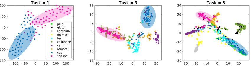
100 100
 Accuracy (%) class iid instance
 80 80 HAMN (ours) 36.8 ± 2 29.6 ± 2
 Top-1 Accuracy (%)

 Top-1 Accuracy (%)
 60 60 HAMN (ours)
 NumMemSlot 27.7 ± 1 27.6 ± 4
 EWC
 GEM
 iCARL
 NumIndexReplays 33.3 ± 2 33.9 ± 6
 40 40 L2
 MAS MemSparseness 35.8 ± 3 33.0 ± 5
 NaiveRehearsal
 20 20 SI
 lowerBound
 DistillationLoss 36.8 ± 4 25.1 ± 3
 upperBound
 0 0
 Chance MemUsageLoss 33.2 ± 5 26.8 ± 5
 1 2 3 4 5 1 2 3 4 5
 Task Number Task Number NoReplay 16.0 ± 1 17.2 ± 1
 (a) class iid (b) class instance
Figure 3: Top-1 classification accuracies over all tasks in class iid Table 1: Top-1 classification accuracies in the
and instance stream learning protocols on CORe50. See Sec 3 for 5th task for the ablated HAMN models after 5
experimental protocols and datasets. See Sec 5.1 for baselines. See runs on CORe50 in the class iid and instance
Supp. material for results on Toybox and iLab. The error bars denote protocols. See Sec. 6.2 for each ablated method.
root mean squared error (RMSE) over total 10 runs. ± value denotes root mean squared error (RMSE).

Figure 4: Clusters of class embeddings learnt in task 1 remain separated in subsequent tasks after hypothesis replays.
We provide t-sne [33] plots of logit vectors from each class after hypothesis replays within a class instance training run on
the CORe50 dataset. Task 1 is a binary classification problem. Tasks 3 and 5 are 1-choose-6 and 1-choose-10 classification
problems respectively. Colors correspond with the object classes in the legend. We use the shaded blobs to emphasize the
clusters of cups and scissors from the 1st task and their corresponding locations in subsequent tasks.
protocols (See Supp. material for the results on the Toybox re-use learnt hypotheses and transfer knowledge from
and iLab datasets). HAMN (dark blue) generally performs previous tasks more effectively. Similarly, the feature maps
better than other continual learning methods in the CORe50 reconstructed from learnt hypotheses and used for replay
(Figure 3) and iLab (Supp. Fig S1c, S2c, and S3c) datasets, seem to carry discriminative information between classes.
and is comparable to the best baseline in the Toybox dataset Finally, compared with parameter regularization methods,
(Supp. Fig S1b, S2b, and S3b). our method is three fold more efficient in memory usage.
 For task 1, all the methods yield approximately the The class instance protocol is more challenging than
same performance, comparable to the upper bound. The class iid, as shown by the performance differences of each
upper bound yields slightly better performance because method between the two protocols (compare Figure 3a
it is trained over multiple epochs whereas all the other and Figure 3b). One reason the performance of HAMN
algorithms are only trained for one epoch. As more tasks are is worse in the class instance setting is overfitting of the
added, performance for task 1 decreases due to forgetting learnt hypotheses to particular tasks. One way to eliminate
(Supp. Fig S5). In task 5, several of the baseline methods hypothesis overfitting is to decrease the hyperparameter
are barely above chance level and are comparable to the controlling the attention strength β, encouraging the
lower bound. The best baseline methods are iCARL, network to use many hypotheses drawn from different tasks
L2, and NaiveRehearsal. Our method (HAMN, dark simultaneously. In an ablation study described below, we
blue) achieves the overall highest classification accuracy show the importance of controlling the attention strength β
among all compared methods (see also Supp. Fig S3a). in the two protocols.
Our method (blue) consistently outperforms the second Figure 4 provides visualizations of the predicted logit
best method (iCARL) across all tasks with an average vectors after hypotheses replays during the class instance
improvement of 7%. This observation reveals that, given protocol. We randomly choose 50 logit vectors from
comparable memory usage with iCARL, our method can each class and project them onto 2D space via t-sne [33].

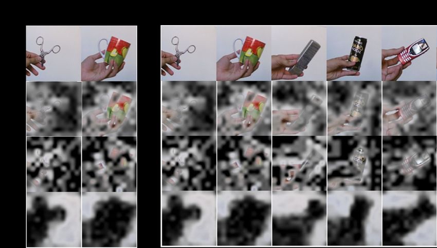
In this example, Task 1 involves separating two classes:
cups and scissors. As expected, the representation of
those two classes is quite distinct, which leads to a high
classification accuracy. In Task 3 and 5, the plots show
the representation of the added classes. Remarkably, the
two initial classes remain distinctly separated despite the
network never training on those classes after the first
task. This shows HAMN accommodates new classes while
maintaining the clustering of previous ones.

6.2. Ablation Study
 We assessed the importance of design choices by training Figure 5: Each hypothesis represents a concept and
and testing ablated versions of the model on CORe50 each learnt concept remains the same across tasks. To
(Table 1). First, we tested the importance of the number visualize what activates each hypothesis in the augmented
of memory slots N by reducing it from N = 100 to memory, given any image It , we used its top-1 attention
N = 50 (NumMemSlot). As expected, there is a drop index tensor wts of size D ×W ×H, selected the hypothesis
in accuracy on the final task of almost 10% and 2% for index of interest, and computed its activation probability
the class iid and class instance protocols respectively. This over all locations, resulting in a 2D probabilistic hypothesis
observation implies that we need a sufficiently high number activation map. We overlaid this map back to image pixels.
of hypotheses to discriminate between classes. The brighter regions denote locations of higher probability
 Second, we halved the number of stored samples (pairs where the selected hypotheses get activated.
of top-1 attention memory indices and their corresponding
 extracted from the feature extractor F (·). There was no
logits) for replay to X = 100 (NumIndexReplays). A
 significant effect of removing the distillation loss for the
moderate accuracy drop of about 5% is observed for class
 class iid protocol; however, there was a drop of 5% in
iid, indicating that the representations of each individual
 classification performance for the class instance protocol.
class are diverse and we need to store multiple samples
 Fifth, in MemUsageLoss, we removed the least used
per class to represent this diversity. Reducing X is not
 memory loss Lmem , which was introduced to prevent
as harmful as reducing N , suggesting that the hypotheses
 useful old hypotheses from being over-written. Removing
in the augmented memory are highly discriminative and
 Lmem results in a 3% accuracy drop for both protocols,
representative and that there exist regularities among
 demonstrating that preventing interference between old and
representations within the same class that reduce the need
 new hypotheses helps prevent catastrophic forgetting.
to store as many replay samples as in pixel-based replay
methods. In contrast, we observed the opposite effect for Lastly, we removed replay from the HAMN model
the class instance protocol, where this ablation improved (NoReplay). As expected, Lmem alone is not sufficient
accuracy by 4%. This suggests that models more easily to avoid catastrophic forgetting. The large decrease
overfit in the class instance setting. in accuracy of 15-20% for both protocols emphasizes
 Third, in MemSparseness, we decreased the reading that replay is essential and demonstrates that replayed
attention strength β ( Eq. 3) from 5 to 1. A higher β forces feature maps constructed from the learnt hypotheses capture
the model to attend to fewer memory slots. Setting β to representative information for old classes.
1 produces a more blurred distribution over all hypotheses,
 6.3. Memory Interpretation
causing an accuracy drop of ≈ 1% in the class iid protocol.
Surprisingly, the lower sparsity helps the model in the class To interprete what learnt hypothesis in the augmented
instance protocol. One conjecture is that HAMN more memory represent, we provide a visualization of 2D
easily overfits in the class instance protocol, so a blurred probabilistic hypothesis activation maps for three
hypotheses distribution could help alleviate the strong hypotheses on an image from each class within a class
preference for a single hypotheses during predictions. instance training run on CORe50 (Figure 5). The brighter
 Fourth, distillation loss is important for knowledge regions denote locations where the hypothesis of interest is
transfer between networks [13] and across sequential tasks more likely to get activated. It is interesting that we find
[28]. We introduced two distillation losses in HAMN: (i) consistent activation patterns over all classes. For example,
during replay with reconstructed feature maps to ensure hypothesis 2 focuses on hand features, hypothesis 6 detects
the network retains discriminative representations for old long edges, and hypothesis 21 prefers the background. We
classes; (ii) during training to ensure the network can also provide a side-by-side comparison of the hypotheses
construct feature maps as representative as maps directly from the same memory index between tasks 1 and 5. We do

not observe a change of hypothesis patterns with new tasks, Neuroscience-inspired artificial intelligence. Neuron,
implying that the learnt hypotheses are not overwritten 95(2):245–258, 2017. 1
by new ones thanks to the least used memory loss Lmem . [11] Tyler L Hayes, Kushal Kafle, Robik Shrestha, Manoj
This is useful to avoid catastrophic forgetting and to Acharya, and Christopher Kanan. Remind your neural
assist transfer learning on new tasks. We also verified the network to prevent catastrophic forgetting. In European
importance of Lmem in the ablation study in Sec 6.2. Conference on Computer Vision, pages 466–483. Springer,
 2020. 1, 2, 3, 5
7. Conclusion [12] Xu He and Herbert Jaeger. Overcoming catastrophic
 interference using conceptor-aided backpropagation. 2018.
We addressed the problem of stream learning for 2
classification tasks by proposing a novel method of memory [13] Geoffrey Hinton, Oriol Vinyals, and Jeff Dean. Distilling
index replay using hypotheses stored in an augmented the knowledge in a neural network. arXiv preprint
memory. In addition to significantly ameliorating arXiv:1503.02531, 2015. 3, 8
catastrophic forgetting on benchmark datasets, our method [14] Forrest N Iandola, Song Han, Matthew W Moskewicz,
features highly efficient memory usage compared to other Khalid Ashraf, William J Dally, and Kurt Keutzer.
 Squeezenet: Alexnet-level accuracy with 50x fewer
methods, while also being generalizable to novel concepts
 parameters and¡ 0.5 mb model size. arXiv preprint
even when trained only once on a continuous stream of data. arXiv:1602.07360, 2016. 5, 6
 [15] Herve Jegou, Matthijs Douze, and Cordelia Schmid.
References Product quantization for nearest neighbor search. IEEE
 [1] Rahaf Aljundi, Francesca Babiloni, Mohamed Elhoseiny, transactions on pattern analysis and machine intelligence,
 Marcus Rohrbach, and Tinne Tuytelaars. Memory aware 33(1):117–128, 2010. 2
 synapses: Learning what (not) to forget. In Proceedings [16] Ronald Kemker, Marc McClure, Angelina Abitino, Tyler L
 of the European Conference on Computer Vision (ECCV), Hayes, and Christopher Kanan. Measuring catastrophic
 pages 139–154, 2018. 6 forgetting in neural networks. In Thirty-second AAAI
 [2] Craig Atkinson, Brendan McCane, Lech Szymanski, and conference on artificial intelligence, 2018. 1
 Anthony Robins. Pseudo-recursal: Solving the catastrophic [17] James Kirkpatrick, Razvan Pascanu, Neil Rabinowitz,
 forgetting problem in deep neural networks. arXiv preprint Joel Veness, Guillaume Desjardins, Andrei A Rusu,
 arXiv:1802.03875, 2018. 2 Kieran Milan, John Quan, Tiago Ramalho, Agnieszka
 [3] Ali Borji, Saeed Izadi, and Laurent Itti. ilab-20m: A Grabska-Barwinska, et al. Overcoming catastrophic
 large-scale controlled object dataset to investigate deep forgetting in neural networks. Proceedings of the national
 learning. In Proceedings of the IEEE Conference academy of sciences, 114(13):3521–3526, 2017. 2, 6
 on Computer Vision and Pattern Recognition, pages [18] Pang Wei Koh and Percy Liang. Understanding black-box
 2221–2230, 2016. 2, 3 predictions via influence functions. In Proceedings of the
 [4] Pratik Prabhanjan Brahma and Adrienne Othon. Subset 34th International Conference on Machine Learning-Volume
 replay based continual learning for scalable improvement 70, pages 1885–1894. JMLR. org, 2017. 5
 of autonomous systems. In 2018 IEEE/CVF Conference [19] Sang-Woo Lee, Jin-Hwa Kim, Jaehyun Jun, Jung-Woo Ha,
 on Computer Vision and Pattern Recognition Workshops and Byoung-Tak Zhang. Overcoming catastrophic forgetting
 (CVPRW), pages 1179–11798. IEEE, 2018. 5 by incremental moment matching. In Advances in neural
 [5] Yutian Chen, Max Welling, and Alex Smola. Super-samples information processing systems, pages 4652–4662, 2017. 2
 from kernel herding. arXiv preprint arXiv:1203.3472, 2012. [20] Zhizhong Li and Derek Hoiem. Learning without
 5 forgetting. IEEE transactions on pattern analysis and
 [6] Jia Deng, Wei Dong, Richard Socher, Li-Jia Li, Kai Li, machine intelligence, 40(12):2935–2947, 2018. 2
 and Li Fei-Fei. Imagenet: A large-scale hierarchical image [21] Vincenzo Lomonaco and Davide Maltoni. Core50: a new
 database. In 2009 IEEE conference on computer vision and dataset and benchmark for continuous object recognition. In
 pattern recognition, pages 248–255. Ieee, 2009. 3, 6 Conference on Robot Learning, pages 17–26. PMLR, 2017.
 [7] Robert M French. Catastrophic forgetting in connectionist 2, 3
 networks. Trends in cognitive sciences, 3(4):128–135, 1999. [22] David Lopez-Paz et al. Gradient episodic memory for
 1 continual learning. In Advances in Neural Information
 [8] Alex Graves, Greg Wayne, and Ivo Danihelka. Neural turing Processing Systems, pages 6467–6476, 2017. 2, 6
 machines. arXiv preprint arXiv:1410.5401, 2014. 2 [23] Davide Maltoni and Vincenzo Lomonaco. Continuous
 [9] Tengda Han, Weidi Xie, and Andrew Zisserman. learning in single-incremental-task scenarios. Neural
 Memory-augmented dense predictive coding for video Networks, 2019. 1
 representation learning. arXiv preprint arXiv:2008.01065, [24] Michael McCloskey and Neal J Cohen. Catastrophic
 2020. 2 interference in connectionist networks: The sequential
[10] Demis Hassabis, Dharshan Kumaran, Christopher learning problem. In Psychology of learning and motivation,
 Summerfield, and Matthew Botvinick. volume 24, pages 109–165. Elsevier, 1989. 1

[25] Cuong V Nguyen, Yingzhen Li, Thang D Bui, and Richard E
 Turner. Variational continual learning. arXiv preprint
 arXiv:1710.10628, 2017. 2
[26] Adam Paszke, Sam Gross, Francisco Massa, Adam Lerer,
 James Bradbury, Gregory Chanan, Trevor Killeen, Zeming
 Lin, Natalia Gimelshein, Luca Antiga, et al. Pytorch: An
 imperative style, high-performance deep learning library.
 arXiv preprint arXiv:1912.01703, 2019. 5
[27] Roger Ratcliff. Connectionist models of recognition
 memory: constraints imposed by learning and forgetting
 functions. Psychological review, 97(2):285, 1990. 1
[28] Sylvestre-Alvise Rebuffi, Alexander Kolesnikov, Georg
 Sperl, and Christoph H Lampert. icarl: Incremental classifier
 and representation learning. In Proceedings of the IEEE
 Conference on Computer Vision and Pattern Recognition,
 pages 2001–2010, 2017. 2, 5, 6, 8
[29] Anthony Robins. Catastrophic forgetting, rehearsal and
 pseudorehearsal. Connection Science, 7(2):123–146, 1995.
 2
[30] Adam Santoro, Sergey Bartunov, Matthew Botvinick, Daan
 Wierstra, and Timothy Lillicrap. One-shot learning
 with memory-augmented neural networks. arXiv preprint
 arXiv:1605.06065, 2016. 2
[31] Hanul Shin, Jung Kwon Lee, Jaehong Kim, and Jiwon
 Kim. Continual learning with deep generative replay. In
 Advances in Neural Information Processing Systems, pages
 2990–2999, 2017. 2
[32] Sebastian Thrun and Tom M Mitchell. Lifelong robot
 learning. Robotics and autonomous systems, 15(1-2):25–46,
 1995. 1
[33] Laurens Van Der Maaten. Accelerating t-sne using
 tree-based algorithms. The Journal of Machine Learning
 Research, 15(1):3221–3245, 2014. 7
[34] Xiaohan Wang, Tengyu Ma, James Ainooson, Seunghwan
 Cha, Xiaotian Wang, Azhar Molla, and Maithilee
 Kunda. The toybox dataset of egocentric visual object
 transformations. arXiv preprint arXiv:1806.06034, 2018. 2,
 3
[35] Junfeng Wen, Yanshuai Cao, and Ruitong Huang. Few-shot
 self reminder to overcome catastrophic forgetting. arXiv
 preprint arXiv:1812.00543, 2018. 2, 5
[36] Jason Yosinski, Jeff Clune, Yoshua Bengio, and Hod Lipson.
 How transferable are features in deep neural networks?
 arXiv preprint arXiv:1411.1792, 2014. 3
[37] Friedemann Zenke, Ben Poole, and Surya Ganguli.
 Continual learning through synaptic intelligence. In
 Proceedings of the 34th International Conference on
 Machine Learning-Volume 70, pages 3987–3995. JMLR.
 org, 2017. 2, 6