IEB Working Paper 2019/03 - TRANSACTION-TAX EVASION IN THE HOUSING MARKET
←
→
Page content transcription
If your browser does not render page correctly, please read the page content below
IEB Working Paper 2019/03

TRANSACTION-TAX EVASION IN THE HOUSING MARKET
José G. Montalvo, Amedeo Piolatto, Josep Raya

                                                          Tax Systems Analysis
IEB Working Paper 2019/03

                  TRANSACTION-TAX EVASION IN THE HOUSING MARKET

                                             José G. Montalvo, Amedeo Piolatto, Josep Raya

The Barcelona Institute of Economics (IEB) is a research centre whose goals are to
promote and disseminate work in Applied Economics, and to contribute to debate and
the decision-making process in Economic Policy.

The IEB research program in Tax Systems Analysis aims at promoting high quality
research in the field of taxation, taking into account not only the traditional approach to
optimal taxation, but also administrative issues and the decentralization or globalization
context. The ultimate aim of the program is to generate socially useful knowledge in
this field. Special emphasis is put on empirical research, and on the analysis of the
Spanish Tax System. The program enjoys the support from the IEB-Foundation.

Postal Address:
Institut d’Economia de Barcelona
Facultat d’Economia i Empresa
Universitat de Barcelona
C/ John M. Keynes, 1-11
(08034) Barcelona, Spain
Tel.: + 34 93 403 46 46
ieb@ub.edu
http://www.ieb.ub.edu

The IEB working papers represent ongoing research that is circulated to encourage
discussion and has not undergone a peer review process. Any opinions expressed here
are those of the author(s) and not those of IEB.
IEB Working Paper 2019/03

           TRANSACTION-TAX EVASION IN THE HOUSING MARKET *

                      José G. Montalvo, Amedeo Piolatto, Josep Raya

ABSTRACT: We model the behaviour of a buyer trying to evade the real estate transfer
tax. We identify over-appraisal as a key, easily-observable element that is inversely related
with tax evasion. We conclude that the tax authority could focus auditing efforts on low-
appraisal transactions. We include ‘behavioural’ components (shame and stigma) allowing
to introduce buyers' (education) and societal (social capital) characteristics that explain
individual and idiosyncratic variations.

Our empirical analysis confirms the predictions using a unique database, where we directly
observe: real payment, value declared to the authority, appraisal, buyers' educational level
and local levels of corruption and trust.

JEL Codes: G21, H26, R21
Keywords: Transfer tax, tax evasion, second-hand housing market, overappraisal, Loan-
To-Value, corruption, social capital, stigma, shame, education

José G. Montalvo                                      Amedeo Piolatto
Universitat Pompeu Fabra-ICREA,                       Universitat Autònoma de Barcelona,
BGSE                                                  Institut d’Economia de Barcelona (IEB),
E-mail: jose.garcia-montalvo@upf.edu                  BGSE & MOVE
                                                      E-mail: amedeo.piolatto@uab.es

Josep Raya
Universitat Pompeu Fabra,
ESCSE (Tecnocampus)
E-mail: josep.raya@upf.edu

*
  Acknowledgements: J. G. Montalvo gratefully acknowledges the financial support of the Spanish
Ministry of Economy and Competitiveness (ECO2017-82696P) and the Government of Catalonia
(ICREA-Academia and SGR2017-616). Amedeo Piolatto acknowledges financial support from the
Programa Ramón y Cajal (RYC-2016-19371). Josep Raya acknowledges financial support from the
Spanish Ministry of Economy and Competitiveness (ECO2016-78816R). Montalvo and Piolatto also
acknowledge the financial support of the Spanish Ministry of Economy and Competitiveness, through the
Severo Ochoa Programme for Centres of Excellence in R&D (SEV-2015-0563) and the Barcelona GSE.
1 Introduction
Real estate transfer taxes are common in most OECD countries and yet
they remain understudied (Best & Kleven 2018). Similarly, the empirical
literature on tax evasion has advanced slowly, mainly due to the challenge
of obtaining reliable data.1 Difficulty understanding and observing fraud
has obvious consequences on the effectiveness of audits performed by tax
authorities. This work aims to help fill these gaps by focusing on home
buyers’ strategic behaviour, whereby we test our prediction and provide
some policy recommendations.
To this end, we present a model where an agent decides their housing ex-
penditure, together with the share of the latter they declare to the tax
authority. The model embeds elements of behavioural economics identified
by the most recent literature on tax evasion as potentially crucial to ex-
plaining tax evasion decisions. In particular, we introduce what we denote
as ‘stigma’, reflecting the dis-utility or unease that an agent may feel when
other people become aware of a fraudulent behaviour; stigma is only suffered
when an agent is caught cheating. In parallel, we also include ‘shame’, which
corresponds here to the feeling of guilt that an agent may suffer, regardless
of whether their fraudulent behaviour is discovered. Both elements depend
on social norms, trust and social capital. Furthermore, shame varies with
individual characteristics such as level of education.
The model uncovers the relation between tax evasion, access to cash (or other
untraceable payment systems) and housing over-appraisal.2 Our result has
an interesting policy implication: as over-appraisal is much easier to observe
than possession of cash or other proxies for fraudulent behaviour, the tax
authority could use it to determine which transactions to audit.
Our paper is thus related to the literature on over-appraisal. This literature
suggests that over-appraisal was a generalised practice during the real es-
tate bubble of the mid-2000s in the U.S. (Nakamura et al. 2010, Ben-David
2011) and in Spain (Montalvo & Raya 2012, Akin et al. 2014, Montalvo &
Raya 2018).3 Nakamura et al. (2010) suggest that appraisals were subject to
1
Alm (2012), Scheneider & Enste (2000), Slemrod & Yitzhaki (2002), Esteller-Moré
et al. (2018) provide extended surveys of the rich literature. Slemrod & Weber (2012)
presents an analysis of the limits to the empirical study of tax evasion.
2
Agents inflate the price of the real estate transaction and expand its scope by adding
items such as appliances, transaction or other costs.
3
Cho & Megbolugbe (1996) and Loebs (2005) provide evidence that in the U.S. the
appraised price is (weakly) above the selling price more than 95% of the time. The figures
in the Spanish market are even higher (Akin et al. 2014). The institutional setting may
play a crucial role relative to both the accuracy of appraisal and incentives to evade the
transfer tax. The U.K. possibly represents the most extreme case documented in the
literature in terms of compliance: appraisal tends to reflect the true value of the property
1an upward bias, such that borrowers were able to obtain larger mortgages,
driving excessively risky mortgage loans.4 In theory, this behaviour should
not be possible, as the (formally independent) appraiser should value homes
objectively (Mae 2007). However, appraisers’ incentives were distorted in
that their clients (money lenders) were often the ones pressuring them to
overstate the value of the property.5 Analogously, in Spain during the hous-
ing boom, most agents underestimated the risks of granting overly generous
mortgages, assuming that house prices would grow without limits. Finan-
cial institutions were prone to open the market to borrowers with financial
constraints. Meanwhile, appraisers were encouraged to upward bias their
valuations, in turn used to produce artificially low LTVs, which ostensibly
kept the credit risk of the mortgage portfolio under control (Montalvo &
Raya 2018). Over-appraisal in Spain reached as high as 29% (Montalvo &
Raya 2012), explained in part by the additional perverse incentive that more
than half of the appraisals were performed by companies directly owned by
financial institutions.
Using a novel dataset, which includes second-hand private housing transac-
tions that occurred in Spain between 2005 and 2011, we test the model’s
results empirically. The data at our disposal is unique in that it includes
both the real transaction price and that declared to the tax authority. Fur-
thermore, for a subset of transactions, we also observe the socioeconomic
characteristics of the buyer and some information about their mortgage.
Furthermore, we are able to observe the level of tax evasion without noise,
and to identify several strong patterns. In particular, we detect a very ro-
bust negative effect of over-appraisal on tax evasion, as predicted by our
theoretical model. We are also able to identify sources of heterogeneity in
tax evasion both at the individual and the geographical level. Indeed, both
stigma and shame seem to matter. We show that tax evasion decreases as
the buyer’s level of education rises while it varies depending on the local
level of law compliance and trust, measured using different indicators of
corruption and trust.
(Cloyne et al. In press), and evasion of the Stamp Duty Land Tax is minimal (Best &
Kleven 2018). In the U.S., an increase in inflated transactions was observed between 2000
and 2006 (Ben-David 2011).
4
The underlying mechanism was the belief that housing prices would continue to grow
strongly, reducing the risk of default. In this scenario, appraisal prices lost validity as
a risk assessment of the mortgage loan and gained validity as an element to be used for
mortgage lending, since a higher appraisal price reduced the LTV ratio. LaCour-Little &
Malpezzi (2003) find a positive association between the quality of appraisals and mortgage
defaults. In a previous study, Lang & Nakamura (1993) note that, in this case, the bank
would require a larger down-payment.
5
The experiment in Freybote et al. (2014) suggests that appraisers were influenced in
their valuation. Although in the U.S., the deviation of the price from the real economic
value was relatively small (6,6% in Ben-David 2011).
2The theoretical model is in line with the long-standing literature that fol-
lows the seminal papers of Allingham & Sandmo (1972) and Yitzhaki (1974),
where evasion has been modelled as a decision made under risk by expec-
ted utility maximising agents. The probability of being audited may de-
pend both on the level of evasion and other idiosyncratic characteristics.6
However, standard models of tax evasion have failed to explain certain em-
pirical regularities. Behavioural economists have consequently augmented
the standard model in different ways.7 The introduction of pro-social beha-
viours, the ‘warm-glow effect’ and feelings of stigma have proved extremely
helpful in efforts to reconcile theoretical predictions and data.8 Our model,
as mentioned, follows this approach and includes both stigma and shame,
which are meant to account for the different possible ‘behavioural’ compon-
ents.
Studying the Spanish case is particularly interesting for at least three reas-
ons. First, the empirical literature places Spain amongst the European
Union countries with the highest levels of tax evasion, with estimates that
range between approximately 20 to 25% of the GDP (Sardá 2014, Scheneider
2005, Medina & Scheneider 2017). Second, across the EU, urban develop-
ment and construction are sectors where corruption vulnerabilities are usu-
ally high (Commission 2014). In Spain, a number of corruption cases related
to these sectors have been investigated and prosecuted in recent years. Fraud
has been closely related to the housing market, particularly during the boom
years. Perhaps the most common form of tax evasion in the housing market
in Spain is under-declaring the purchase price to the tax authority. In this
way, buyers reduce the burden of the real estate transfer tax, while sellers
pay less taxes on capital gains. Finally, the strong ties between financial
institutions and appraising firms and the volatility of the economy during
the analysed period potentially leave more room for variation and thus allow
to better identify different behavioural patterns.
The remainder of the paper is organised as follows. Section 2 presents the
theoretical model that explains the evasion of the real estate transfer tax.
The model’s predictions are tested in Section 3 using a unique dataset on
Spain that includes observations on real estate transactions from 2005 to
2011. We begin by describing the institutional setting in Section 3.1, then
6
We abstract from the analysis of how the tax authority optimally sets the probability of
audit. For more on this, see Reinganum & Wilde (1985), Macho-Stadler & Pérez-Castrillo
(1997), Chander & Wilde (1998), Di Porto et al. (2013), Piolatto & Trotin (2016).
7
A broad literature has developed around the idea of agents who follow the tenets of
prospect theory. See, for example, Bruhin et al. (2010), Alm (2012), Hashimzade et al.
(2013), Engström et al. (2015), Piolatto & Rablen (2017).
8
Such additions may include aspects such as stigma (Gordon 1989, Kim 2003), social
norms (Traxler 2010), intrinsic motivation like duty or tax morale (Dwenger et al. 2016),
equity, fairness or trust (Bordignon 1993, Falkinger 1995, Schildberg-Hörisch & Strassmair
2012).
3present the data in Section 3.2, followed by our results in Section 3.3. Finally,
Section 4 concludes. Proofs can be found in Appendix A, while several
complementary tables are included in Appendix B.
2 Model
We consider a representative consumer, who cares about the consumption
of housing and of a numeraire good. When purchasing a house, the agent is
obligated to declare it to the tax administration and to pay an ad valorem
transfer tax. However, the agent may under-declare the value of the trans-
action in order to reduce their tax liability. In doing so, the agent may incur
an administrative sanction. Moreover, she may suffer some disutility from
misbehaving.
The expected utility function of the agent is defined as
E(U ) = h(H) + E(C) − π (H u , e) s − µ (H u , θ, n) , (1)
where H represents the value of the housing.9 E(C) is the expected value
of consumption of the numeraire good. π is the (perceived) probability of
getting caught by the tax administration and is an increasing function of
the amount H u that is hidden from the tax administration and of the idio-
syncratic enforcement level e, while s represents the stigma that the agent
suffers when caught. Finally, µ represents individual moral shame/guilt
suffered regardless of whether one is caught, which is a function of the level
of evasion H u , of individual characteristics θ (education) and of how socially
unacceptable is to evade n. We assume that h(H) is increasing and concave
in H and that the probability of getting caught π is increasing and concave
in the amount evaded: h0 (H) > 0, h00 (H) < 0, πu0 > 0, πu00 < 0. We also
assume moral shame to be increasing in the amount evaded, µ0u > 0, and
∂2µ ∂2µ
that ∂H u ∂θ > 0 and ∂H u ∂n > 0. These two assumptions on the crossed de-
rivative are quite natural (we expect both more educated people to be more
respectful of the law and shame to increase in environments where society
doesn’t tolerate evasion), and are fully supported by the empirical analysis.
The agent has some ‘liquid’ savings L, where liquidity is interpreted as
money that can be hidden from the tax authority (for example, cash or
bitcoins). We normalise to 0 the amount of savings that the agent is unable
9
For notation convenience, H is the monetary value of the house. If we denote by q
the per square-metre price and by Ĥ the number of square-metres, then H = q Ĥ. For the
purposes of this analysis, note that we can directly work with H without consequences,
as long as we do the same with H d (the value that is declared to the tax authority) and
with H u (the value that is hidden from the tax authority). This simplification is possible
because we don’t study the consequences of market prices.
4to hide. The agent is able to borrow an amount B against some value I
that can be interpreted as the net present value of future income or some
collateral. Then, E(C) = I − (1 + i)B − πf H u , where i is the interest rate
on borrowing, while f is the fine rate that is paid if caught cheating.
By construction H = H d + H u ; H d is the part of the housing value that is
declared. Furthermore, we impose that H u ≤ L, that is, borrowed money
cannot be hidden from the tax authority. Finally, denoting t as the transfer
tax on the declared housing value, restriction (1 + t)H d + H u ≤ L + B
guarantees that the agent spends on housing at most all their savings plus
borrowing. Since borrowing money is costly, it is never optimal to borrow
more than what is needed to purchase the house, therefore we can rewrite
the previous restriction as B = (1 + t)H d + H u − L. Notice that, at any
interior solution, this model is isomorphic to a two-period model in which
the agent in period 1 borrows from period 2 and purchases the house, while
in period 2 they pay back the debt and consume the numeraire good.
Using H = H d + H u , we can rewrite B = (1 + t)H − tH u − L. We assume
the interest rate to be an increasing
convex function
of the loan to value. In
u −L
particular, we assume i HBd = i (1+t)H−tH , with i0 > 0 and i00 > 0.
H−H u
The maximisation problem of the agent is then
max h(H) + I − (1 + i) ((1 + t)H − tH u − L) − π(f H u + s) − µ, (2)
H,H u
which yields to the first order conditions (FOCs):
(L − H u ) ((1 + t)H − tH u − L)
h0 (H) =i0 + (1 + i)(1 + t) (3)
(H − H u )2
(H − L) ((1 + t)H − tH u − L)
(1 + i)t =i0 + πu0 (f H u + s) + πf + µ0u (4)
(H − H u )2
The FOCs represent the maximum of the objective function if the problem
is well-behaved. The following lemma defines the conditions under which
this is the case.
Lemma 1 (Second order conditions). The second order conditions (SOCs)
are satisfied if and only if ψ > ψ, where ψ = πu00 (f H u + s) + 2πu0 f + µ00u ,
h00 (H)(H−L)2 φ
ψ= (L−H u )2 φ−h00 (H)(H−H u )3
and φ = i00 HBd + 2i0 .
Proof. See appendix A.
Eqs. (3) and (4) together define implicitly the optimal level for the two
control variables H and H u . Applying the implicit function theorem on the
system of equations, we can study how the parameters of the model influence
5the control variables. For this, we denote the first order conditions, Eqs. (3)
and (4), respectively as F1 = 0 and F2 = 0.
We start by looking at the impact of liquid savings L and obtain that
∂F1 ∂F2
∂H ∂H u ∂L − ∂F 1 ∂F2
∂L ∂H u
= (5)
∂L D(H, H u )
and
∂H u − ∂F1 ∂F2 + ∂F 1 ∂F2
= ∂H ∂L ∂L ∂H
(6)
∂L D(H, H u )
where D(H, H u ) > 0 is the determinant of the Hessian matrix.10 The pre-
vious equations simplify to
∂H (L − H u )(H − H u )φψ
= (7)
∂L D(H, H u )
and
∂H u −h00 (H)
= >0 (8)
∂L D(H, H u )
Notice that the sign of Eq. (7) depends on the sign of ψ, which could admit
both positive and negative values. When the theoretical analysis remains
ambiguous about the sign of the derivative, we must check the data to
clarify the impact of L on the total consumption of housing. Our empirical
analysis thus helps to answer this question, as well as confirms the result
that an increase in liquidity, as expected, leads unequivocally to an increase
in evasion.
At this point in the analysis, it becomes convenient to introduce two new
variables: V and Ṽ = HVd . The former denotes the appraisal value, that is,
the estimation of the value of the property realised by the financial institu-
tion that provides the loan. The latter is instead a measure of over-appraisal,
which takes values above 1 when the financial institution appraises the prop-
erty higher than its declared value. It is interesting to use over-appraisal
for several reasons. First of all, there is an empirical literature suggesting
a relation between over-appraisal and tax evasion. Second, over-appraisal
is a measure that is easily observable by the tax authority, as opposed to
evasion and liquid savings, which are harder to detect. Should we be able to
identify a link between over-appraisal and evasion, the tax authority could
use this as a proxy to identify cases where it is more likely that some eva-
sion took place. Finally, there are often restrictions on how much an agent
can borrow, which depend on the appraisal value. Since the appraisal is, in
many countries, directly computed by the financial institution, there is an
incentive to distort the value V , if need be.
10
The explicit expression for D(H, H u ) is provided within the proof of Lemma 1.
6Assume that the financial institution can lend at most a percentage α of V ,
which is often the case. The agent will then pushu the financial institution
−L
to set V such that B = αV , hence V = (1+t)H−tH α . Then, α becomes a
measure of how much an agent will be allowed to borrow, which may depend
on the legal setting, on individual characteristics and also possibly on some
exogenous macroeconomic factors (e.g. GDP or unemployment).
∂ Ṽ (H − H u )h00 (H)
L(H − H u )2 + (H − L)2 φ + (H − H u )3 ψ
= u
(9)
∂L D(H, H )
2 u )2
It is simple to check that ∂∂L
Ṽ
< 0 if and only if ψ > − (H−L)(H−H
φ+l(H−H
u )3 ,
which is always the case under the regularity condition that ψ > ψ.
The following proposition puts together the results on the impact of a change
in L, leading to our first policy implication and empirical question.
Proposition 1. An increase of the liquid savings L induces an increase in
u
the amount of undeclared housing, ∂H ∂L > 0, and a decrease in the observed
over-appraisal, ∂∂L
Ṽ
< 0. The effect of L on the total amount of housing, ∂H
∂L ,
is instead unclear and must be tested empirically.
Proof. See appendix A.
Corollary 1. An increase in the amount of savings that can be hidden from
the tax authority (which is usually not observable) has opposite effects on
tax evasion and over-appraisal. Therefore, the data should show a negative
correlation between the level of evasion and over-appraisal. Since the latter is
usually much easier to observe, this correlation can be used as an indicator
of a possible fraud. Our empirical analysis indeed confirms the negative
correlation between evasion and over-appraisal.
Corollary 2. In order to assess how liquid savings affect the total expendit-
ure on housing H, we can also look at whether housing H and over-appraisal
Ṽ are positively or negatively correlated. This allows to uncover the sign of
∂H
∂L . If and only if H and Ṽ are negatively correlated, we conclude that
∂H
∂L > 0.
The logic behind Proposition 1 and Corollary 1 is straightforward: the
amount of available liquid savings is crucial to determine how much an
agent is able to evade. Meanwhile, any liquidity constraint has an impact
on the amount that an agent needs to borrow. As a consequence, an agent
with access to liquid savings can afford to evade and doesn’t need to push
for over-appraisal, whereas a liquidity-constrained agent is unable to evade
and must furthermore ask for an over-appraisal. It consequently follows that
the level of evasion and over-appraisal are negatively correlated. This has
7a clear and important policy implication: tax authorities should focus their
efforts on preventing evasion by auditing transactions that show low levels
of over-appraisal.
In the literature on tax evasion, there has appeared a growing interest in
the role of behavioural components, such as stigma, in the decision to evade
taxes (see the introduction for references). In our model, we introduced two
distinct behavioural features. We denoted as stigma the dis-utility that an
agent suffers when they are caught cheating.11 We also consider the moral
shame that an individual feels when they cheat. This element differs from
stigma in that an individual is always aware of having cheated and hence a
sentiment of guilt is present regardless of whether she is caught. Shame is
imposed by society and, as such, depends on the latter’s level of morality.
It is, in addition, agent-specific, and thus also depends on individual char-
acteristics (e.g. education). Finally, stigma is a binary variable, in the sense
that people will mostly remember the scandal but not the details. Shame,
being an individual feeling, depends on the level of evasion: an individual’s
guilt will grow with the amount evaded.
Proposition 2. In this model, at any interior solution, stigma plays a role
on the level evaded only as long as the probability of getting caught depends
∂π
on the amount evaded. When ∂H u = 0 stigma may deter evasion (corner
solution) but it does not affect the level of evasion, conditional on evading.
u
As expected, the level of evasion is negatively affected by stigma: ∂H ∂s < 0.
Proof. See appendix A.
Proposition 2 suggests that the role of stigma, as defined here, is limited to
when the probability of being caught depends on the level of evasion. The
intuition is that stigma only matters if one gets caught. If the probability
of being caught is orthogonal to the agent’s behaviour, then stigma will
only determine the extensive margin (the probability of evading) but not
the intensive margin (how much to evade).
The decision to evade taxes is certainly affected by both the surrounding
environment (e.g. the level of tax enforcement and the moral code of a
society) and by individual characteristics (e.g. the level of education). In this
model, the environment may enter through two channels (on top of stigma,
which has already been discussed): it may directly affect the probability of
being caught, through the level of enforcement e, or it may affect the level
of shame, through n. Individual characteristics θ, instead only affect the
model through shame. Proposition 3 discusses both of these elements.
Proposition 3. The housing value that is hidden from the tax authority may
vary locally, depending on the level of enforcement e and, through shame,
11
The idea being that society cannot stigmatise a tax evader if the latter is not caught.
8on how much tax evasion is socially disapproved of n. As one may expect,
u ∂H u
both factors negatively affect the level of evasion: ∂H
∂e < 0 and ∂n < 0.
Furthermore, law compliance varies at the individual level, through shame,
u
due to individual characteristics θ (such as education), so that ∂H
∂θ < 0.
Proof. See appendix A.
Proposition 3 confirms that society has an impact on the individuals’ de-
cision to evade. Indeed, the perceived enforcement affects the decision of
a rational individual. Furthermore, living in a society that is less tolerant
towards illegal behaviour produces more shame, which reduces the level of
evasion. The empirical analysis confirms this result, showing that more eva-
sion is observed in regions with higher levels of corruption and where social
values are lower. Individual characteristics also matter: when the parameter
θ increases, the level of evasion decreases. We also test this in our empir-
ical analysis, where we observe that more educated agents are less prone to
evasion.
The empirical analysis allows us to relate evasion with changes in macro-
economic factors such as GDP or unemployment. While such parameters
are not directly present in our theoretical model, we could expect some of
our variables to be affected by them. In particular, a decrease in GDP or an
increase in unemployment may affect, on average, our variable L. Should
this be the case, we would expect a decrease in GDP to reduce the level of
evasion H u . Macro-economic factors such as GDP and unemployment may
also have an impact on the availability of credit, which in turn could affect
the variable α (the share of the valuation that an agent can borrow). Notice
B ∂ Ṽ B
that Ṽ = αH d , thus, ∂α = − α2 H d < 0. Therefore, since α is negatively
correlated with over-appraisal, a credit restriction would tend to increase
the tendency to over-appraise properties.
3 Empirical analysis
In this section, we test the previous results using a novel dataset on about
1,500 real estate transactions that occurred in Spain during the period 2005-
2011. The dataset is particularly unique in that it includes both the value
declared to the tax authority and the amount effectively paid. In what
follows, we begin by presenting the institutional framework, we then describe
our data and finally, report the results.
93.1 Institutional framework
Over the first decade of the twenty-first century, Spain experienced one of
the largest housing booms of any developed economy.12 The construction
sector alone was responsible for approximately 20% of the GDP growth. This
housing boom led to a housing price bubble (housing prices tripled between
1998 and 2008) that began to burst in 2008. At the time, an average of
approximately 1.1 million mortgages per year were approved.13
The lending market was extremely competitive. Spanish financial insti-
tutions offered the lowest mortgage rates of the Euro area. In fact, over
the 2003-06 period, the average mortgage rate in the Euro zone was 21%
higher than in Spain. Financial institutions attempted to compensate for
the reduced per-mortgage margin with an increasing number of transactions,
which contributed to the sharp increase in the number of mortgages. The
excessive dependence of the Spanish economy on the real estate market, to-
gether with loose credit standards (Akin et al. 2014), largely explain why
the financial crisis hit Spain more severely than most other economies.
The attempt to increase the number of transactions led to a softening of
credit standards. Yet financial institutions were constrained by internal
policies on the LTV ratio. These constraints were relaxed by pushing ap-
praisers to over-value properties whenever the borrower did not have suf-
ficient resources for the down-payment or preferred to borrow more for a
different reason. Montalvo & Raya (2018) find evidence consistent with fin-
ancial intermediaries encouraging appraisal firms, most of them owned by
banks themselves, to introduce an upward-bias in their valuations by ap-
proximately 30% to meet the LTV recommendations, so as to be able to
use them as collateral for covered bonds (the limit LTV for this pool of col-
laterals is 80%) and to reduce their capital requirements. Indeed, 40% of
mortgages in the researchers’ sample are bunched at the LTV threshold.
It is important to note that Spain has only been a democracy since 1975.
Young democracies are particularly vulnerable to illegal activities (Treis-
man 2000) and it is well known that different kinds of criminal behaviour,
from tax evasion to black markets and corruption, are positively correlated
(Fortin et al. 2000). It is perhaps not surprising then that Spain ranks third
in Europe in terms of the percentage of citizens (95%) who believe that cor-
ruption is widespread (Commission 2014). Various cases of corruption have,
12
During this period, more dwellings were built in Spain than in Germany, France and
Italy put together. According to the official statistics of the Department of Public Works,
housing initiations reached as high as 860,000 dwellings in 2006.
13
Note that there were approximately 15.5 million households in Spain. Over the con-
sidered period, the average number of transactions realised per year and region was ap-
proximately 20,000, with a standard deviation of about 14,700.
10in fact, recently been uncovered, many of which relate to the real estate sec-
tor and involve politicians at all levels.14 Real estate transfer taxes in Spain
are at the order of magnitude of 10% of the declared value.15 The most
common way to reduce the tax burden related to real estate transactions is
to under-declare the transaction value to the tax authority. The seller may
also occasionally benefit if the sale is classified as speculative and, therefore,
subject to the capital gain tax.
3.2 Our data
Data on either on the Spanish housing boom or related aspects is scant. One
of the main reasons is a lack of reliable statistical information on housing
values. Indeed, prior to 2007, the Spanish house price index was computed
based on appraisals, which were highly unreliable, as mentioned earlier.
Since 2007, the price index has been based on the Property Registry values,
that is, the transaction value declared by the tax payer. As we will show,
this does not correspond to the actual market price either.
Our dataset is the first to include actual market prices. For one-fourth of
the dwellings in the sample, we also have individual characteristics of the
mortgagor. This unique dataset was obtained from a real estate interme-
diary16 that operates across most Spanish provinces and that also runs its
own mortgage brokerage business. The intermediary has a 3-5% market
proportion of realised sales (depending on the year).17
We merged the dataset obtained from the real estate intermediary with
information from other sources. Data from the intermediary include the
actual transaction price (i.e. the amount effectively paid by the buyer, and
on which the intermediary computed their fees), and the characteristics of
the properties from a random sample of their sales. We obtained inform-
ation on the amount of the mortgage, the appraisal value and the buying
price declared to the tax authority from the Property Registry (Registro
de la Propiedad ). To guarantee the correct matching of data, we also ob-
tained the cadastral reference (referencia catastral, a unique identifier for
14
Corruption and illicit practices are common in urban planning and spatial develop-
ment in Spanish cities. Benito et al. (2015) cite 676 cases of urban corruption that have
been documented in the media. Of the corruption cases that occurred during the period
of analysis, some relate to the illicit funding of political parties, or tax fraud and embez-
zlement by members of the government.
15
Contrary to the U.K., where the tax rate increases with the value of the property
(Best & Kleven 2018), in Spain the tax rate is flat.
16
We signed a non-disclosure agreement prohibiting the disclosure of the company’s
name.
17
Notice that most of the existing home sales in Spain are sold directly by the owner.
11each property) from the cadastre (catastro).18 The sample period runs from
2005 to 2011. The merged data allow to compute the amount that was not
declared for 1,445 transactions of existing housing units (apartments). We
refer to this set of data as the ‘whole sample’.
For a subset of 430 observations, we were able to merge previous data with
information provided by financial intermediaries. Thus, this subset includes
individual characteristics of the buyer, such as the number of owners of the
property and their respective levels of education. We refer to this subset
as the ‘sample with individual characteristics’. For these 430 observations,
certain financial information (e.g. appraisal prices or the amount of the
mortgage) was present in several different datasets. We used such redundant
information as a further check of the reliability of the merging process.
Nearly half of the transactions included some undeclared money, with a
mean value for the percentage of undeclared money of 7.64%. Conditional
on fraudulent behaviour, this percentage rises to 15.1%. Figure 1 presents a
histogram of the percentage of undeclared money, including and excluding
zeros. The percentage of undeclared money over the actual selling price was
lower than 20% in 76.03% of the fraudulent transactions.
15
50
40
10
30
Percent
Percent
20
5
10
0
0
0 .1 .2 .3 .4 .5 .6 .7 .8 0 .1 .2 .3 .4 .5 .6 .7 .8
proportion undeclared money proportion undeclared money
Figure 1: Histogram of the proportion of undeclared money
The period we analyse saw both a bubble and a burst in the housing market,
which also had an impact on GDP, unemployment and the economy in
general. Table 1 shows the evolution of tax evasion from 2005 to 2011.
The share of fraudulent transactions steadily decreased over the considered
period. However, note that around 2008 and conditional on fraud, the share
that remained undeclared begins to increase. One possible interpretation,
18
Difficulties matching the data unfortunately caused the loss of some information.
Indeed, the Spanish registry is organised in the format of a ‘continuous roll’: successive
owners of a given property are sequentially added on a single document recorded by
the original address at the time of building. However, due to many political upheavals
(including two dictatorships, the republic and two monarchies), street names have changed
several times over the last century. In order to match the data, it was necessary to match
the address of the estate at the moment of construction with that when it was sold.
12consistent with the discussion at the end of Section 2, is self-selection. When
the crisis hit, many citizens were impoverished. The decrease in GDP and
the increase in unemployment resulted in less buyers having some liquid
savings to use for purchasing. The probability of having sufficient savings to
make any cash side-payments decreased. Meanwhile, the decline in housing
prices that followed the bubble burst meant that agents who had access to
liquid savings could use them to pay a larger share of the total value. To
this regard, Section 3.3 shows how the share of fraudulent transactions is
decreasing in unemployment, while the share that is undeclared (conditional
on fraud) is increasing in unemployment.
Year Transactions with Undeclared Undeclared money,
undeclared money money conditional on fraud
(share) (share) (share)
2005 80.89% 12.59% 14.17%
2006 66.07% 9.58% 14.50%
2007 59.77% 7.91% 13.23%
2008 48.24% 7.34% 15.21%
2009 38.67% 6.13% 15.86%
2010 34.72% 6.24% 17.97%
2011 31.15% 6.73% 21.62%
Source: Own elaboration.
Table 1: Evolution of the undeclared money over time.
Agents’ behaviour proved to be very heterogeneous across the country. Table
2 presents these differences among the regions most represented in the
sample. We immediately observe a spread of up to 23 percentage points
in terms of the share of illegal transactions carried out. Similarly, condi-
tional on fraud, the share of the price that remains undeclared varies from
about 10% (Aragon) to about 19% (Valencian C.).
Table 10, in appendix B displays the descriptive statistics of our dataset
both for the ‘whole sample’ and for the ‘sub-sample with individual char-
acteristics’. The ‘average buyer’ in the sample is employed, has attained
a primary education, buys on their own and obtains a mortgage that is
over-appraised by approximately 30%, with a spread of 0.86.
3.3 Results
In this section, we test the predictions of the theoretical model. For each
specification, we estimate a Probit model for the determinants of the prob-
ability of a fraudulent transaction (that is, under-declaring money to the tax
13Region Transactions Undeclared Undeclared e,
with fraud money condit. on fraud
(share) (share) (share)
Andalusia 59.36% 10.90% 18.36%
Aragon 44.07% 4.53% 10.27%
C. La Mancha 41.86% 6.38% 15.23%
C. León 41.38% 7.26% 17.54%
Catalonia 37.59% 5.27% 14.01%
C. Madrid 53.51% 6.97% 13.03%
Valencian C. 61.80% 11.84% 19.15%
Source: Own elaboration.
Table 2: Distribution of the undeclared money across regions.
authority), as well as a Tobit model for the determinants of the proportion
of undeclared money (that is, the percentage of the total transaction value
that is hidden from the authority).
Proposition 1, together with Corollaries 1 and 2, predicts that over-appraisal
(or LTV) and tax evasion are inversely related. It is left to the empirical
analysis to clarify whether total house spending is positively or negatively
correlated with over-appraisal, which would allow to infer the underlying
relation between liquid savings and house spending. Table 3 confirms the
prediction of the theoretical model and shows that tax evasion and over-
appraisal are strongly, negatively related.
Indeed, we observe in Table 3 that increasing over-appraisal by one point
(that is, the appraisal value doubles the selling price) decreases the probabil-
ity of fraud by 20.94% and decreases the proportion that remains undeclared
by 15.9 points. Using the 29% mean over-appraisal in Spain computed in
Akin et al. (2014), our results suggest that over-appraisal is responsible for a
reduction of 4.6 points in the amount that is hidden from the tax authority.
Complementing the discussion following Proposition 1, buyers try to min-
imise over-appraisal and the amount that they borrow. The use of over-
appraisal to increase the amount that can be borrowed is a last recourse
for a buyer, used only when they have no other alternative. Over-appraisal
becomes a signal of liquidity constraint, which is unlikely to occur for agents
who have liquid savings that can be used for side-payments. Table 3 thus
confirms the model’s prediction and, accordingly, has a strong policy im-
plication. Since over-appraisal is much easier to assess and observe than
access to liquid savings or fraud, it should be used as an indicator for the
likelihood of fraud. In particular, the tax authority should focus their audit
efforts on transactions where the appraisal is relatively low. Results using
the sub-sample with individual characteristics reinforce the argument that
14Whole Sample with
sample individual characteristics
Probit Tobit Probit Tobit
Overappraisal -0.838*** -0.159*** -1.787*** -0.246***
Transactions (thousand) 0.020** 0.001
Spread -0.260 -0.043
Educational level (ref: Primary)
Secondary -0.491* -0.076***
Graduate -0.732** -0.076**
Number of holders (ref: One)
Two 0.207 0.031
Three or more 1.696*** 0.057
Employment (ref: Non-Occupied)
Occupied in private sector -0.410 -0.087*
Occupied in public sector 0.033 -0.055
Self-employed 0.056 -0.005
Intercept -0.623 0.092 2.206** 0.446***
N. Obs. 1.445 430
Year F.E. Yes Yes
Region F.E. Yes Yes
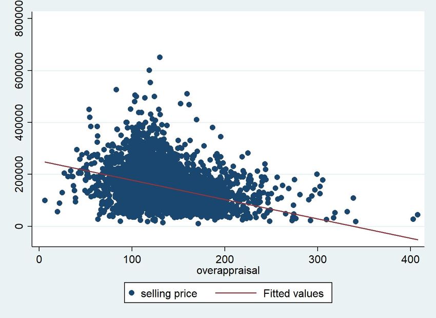
* pFigure 2: Correlation between Total Spending and Over-Appraisal
probabilities. As we do not, unfortunately, have access to such data, it is
not possible test this prediction, which could explain part of the regional
differences in levels of evasion.
It has been well documented19 that a social component that involves in-
formation, trust, social capital, and that we identify here as a stigma, is
responsible for people restraining themselves from acting illegally. To this
regard, our data allows to explain idiosyncratic differences by showing that
the environment and social values indeed explain part of the variance in
fraudulent behaviour. That said, we are unable to distinguish between the
different channels identified in Propositions 2 and 3, namely stigma, audit
probability and shame.
Table 4 shows how evasion varies from one region to another. We ob-
serve that Andalusia and the Valencian Community are the regions with
the highest probability of fraud. Moreover, in these two regions, the pro-
portion of the amount undeclared is also higher than elsewhere.20 The
quantitative interpretation of the Probit results originates from marginal
effects; for these two regions, the probability of under-declaring money in-
creases by 0.34 and 0.29 points, respectively.21 In addition, in Andalusia and
the Valencian Community, the proportion of undeclared money is 14 points
19
See, for example, (Alesina & La Ferrara 2000, Alesina & Ferrara 2002, Boffa et al.
2016) and the literature therein.
20
Note that in the estimation using the sample with individual characteristics, the Com-
munity of Madrid presents a probability of fraud that is significantly higher than the mean,
as is the proportion of the total value that is hidden from the tax authority.
21
Considering a mean probability of 51%, these effects represent an increase close to
70% and 60%, respectively.
16Whole Sample with
sample individual characteristics
Probit Tobit Probit Tobit
Region
Andalusia 1.479*** 0.142*** 1.099** 0.122**
Aragon 0.360 -0.005 0.629 0.067
Castile La Mancha 0.756 0.062
Castile and León 0.328 0.040
Catalonia -0.216 -0.014 0.640 0.064
Community of Madrid 0.473 0.042 1.001** 0.105**
Valencian Community 1.316** 0.139** 2.770*** 0.350***
Overappraisal -0.838*** -0.159*** -1.787*** -0.246***
Transactions (thousand) 0.020** 0.001
Spread -0.260 -0.043
Intercept -0.623 0.092 2.206** 0.446***
N. Obs. 1.445 430
Year F.E. Yes Yes
Individual controls No Yes
* pcipalities, we identified at least one case of corruption. We considered only
the ‘whole sample’ and replaced regional dummies with municipal ones. The
first two columns in Table 5 summarise our results.
Corruption index
(1) (2)
Probit Tobit
Corruption 0.823*** 0.091***
Overappraisal -0.810*** -0.159***
Year (ref: 2011)
2005 2.630** 0.131*
2006 1.547*** 0.113***
2007 1.113*** 0.064*
2008 0.705** 0.046
2009 0.210 -0.005
2010 0.040 -0.008
Transactions (Thousand) 0.005 -0.007
Intercept -0.118 0.120***
N. obs 1.233
* p1,445 observations in our ‘whole sample’, 1,115 overlap with a municipality
covered by the GTI. This robustness test23 confirms our results: we observe
more fraudulent transactions (both on the extensive and intensive margin)
in more corrupt areas. In particular, an increase in one point of either the
GTI or the GTI-Urban index reduces the proportion of the value that is
undeclared by 0.2 points.24
The level of trust and morality of a society is, of course, more than a reflec-
tion of the degree of corruption of its politicians. We consequently tested
our prediction using other indicators of social capital. More specifically, we
used two other indicators of social transparency, corruption or cheating be-
haviour: Table 6 summarises the results. Columns 1-2 are computed using
the Quality of Government (QoG) data from the Quality of Government In-
stitute; in particular, we used the corruption variable (data available at the
regional level). Columns 3-4 use the European Social Value (ESV) index.
The European Values Study is a large-scale, cross-national, longitudinal sur-
vey research programme on basic human values. The study provides insights
into the ideas, beliefs, preferences, attitudes, values and opinions of citizens
across Europe. Specifically, we exploit the question ‘justify cheating on tax’
and compiled this information for every Spanish region for both the 1999
and 2008 waves. We use their difference as a proxy for the changes in tax
evasion behaviour. In all columns, a higher index value means less social
values (columns 1-2)25 , or that tax evasion is more tolerated (columns 3-4).
Again, the results are significant and their sign is that predicted by the the-
oretical model and in accordance with those obtained using different proxies
for stigma and shame.
Alm et al. (2004) and Alm & Torgler (2006) find a negative correlation
between tax morale and the size of the shadow economy. We use data from
Sardá (2014)26 on the mean shadow economy in Spain from 2004 to 2011
at the province level, merging the latter with our dataset. For 1,432 of
the observations in our ‘whole sample’,27 we use the estimated percentage
23
Columns 1-2 of Table 11 depict the results using the adjusted GTI as the measure
of corruption, while columns 3-4 depict the results using the adjusted GTI sub-index
‘transparency in urban planning and public works’ (GTI-Urban).
24
Results are robust to transparency and corruption data aggregation at the provincial
level.
25
In this case, we used the inverse of the original index in the estimation.
26
To measure the size and development of the shadow economy, we adopt a ’Multiple
Indicators Multiple Causes’ (MIMIC) approach (Weck-Hanneman & Frey 1985), a special
case of the general LISREL model. A MIMIC model consists of two parts, the structural
equation and the measurement equation system. The structural model examines the
relationships between the latent variable (output of the shadow economy) and the causes,
while the measurement model links indicators and the latent variable.
27
Sardá (2014) do not report the estimation of the shadow economy for Vizcaya
19QoG Euro. Social Values
(1) (2) (3) (4)
Logit Tobit Logit Tobit
Absence of Social values 0.005 0.0012*** 0.0084** 0.0005
Overappraisal -0.714** -0.151*** -0.714** -0.151***
Transactions 0.00604 0.000417 0.00466 -0.000337
2005 2.650* 0.132 2.564* 0.133
2006 1.261*** 0.0785* 1.306*** 0.0935**
2007 1.057*** 0.0609 1.022** 0.0599
2008 0.686* 0.0432 0.638* 0.0397
2009 0.288 0.00509 0.247 0.00237
2010 0.0826 -0.0118 0.0944 -0.00578
Intercept 0.439 0.214*** 0.126 0.153***
Constant 0.194*** 0.195***
N. obs 1.440 1.445
* pProbit Tobit
Shadow economy (%) 0.069*** 0.012***
Overappraisal -0.735*** -0.153***
Year (ref: 2011)
2005 2.586** 0.121*
2006 1.236*** 0.074**
2007 1.117*** 0.064*
2008 0.681** 0.040
2009 0.268 0.001
2010 0.044 -0.017
Transactions (1.000) 0.008 0.001
Intercept -1.059 -0.088
N. obs 1.432
* pWhole Sample with
sample individual characteristics
Probit Tobit Probit Tobit
Overappraisal -0.838*** -0.159*** -1.787*** -0.246***
Transactions (thousand) 0.020** 0.001
Year (ref: 2011)
2005 2.422** 0.109 0.000 -0.008
2006 1.301*** 0.087** 1.406** -0.005
2007 1.090*** 0.058* 0.295 -0.134**
2008 0.732** 0.041 0.315 -0.055
2009 0.305 0.000 -0.013 -0.068
2010 -0.115 -0.033 -0.772 -0.163***
Spread -0.260 -0.043
Educational level (ref: Primary)
Secondary -0.491* -0.076***
Graduate -0.732** -0.076**
Number of holders (ref: One)
Two 0.207 0.031
Three or more 1.696*** 0.057
Labour situation (ref: Non-Occupied)
Occupied in private sector -0.410 -0.087*
Occupied in public sector 0.033 -0.055
Self-employed 0.056 -0.005
Intercept -0.623 0.092 2.206** 0.446***
Region F.E. Yes Yes
N. Obs. 1.445 430
* pFraud Fraud
Extensive margin Intensive margin
(1) (2)
Unemployment -0.033*** 0.003***
(0.007) (0.001)
Intercept 0.439*** 0.111***
(0.107) (0.009)
N. obs 1445 730
* pant in explaining tax evasion. Previous literature on household borrowing
and mortgages has shown that LTV is a crucial element that heavily affects
constrained borrowers (Di Maggio et al. 2017, Ganong & Noel 2018, Cloyne
et al. In press). Yet, to the best of our knowledge, this is the first paper
that estimates its impact on tax evasion. Interestingly, tax evasion reduces
the effective tax rate and, according to our interpretation of the results,
less constrained borrowers are those who are more likely to evade. Evading
the transfer tax thus has a clear regressive effect in terms of inequality and
redistribution, going against what would be desirable. As shown in Best &
Kleven (2018), ideally the tax should be lower for constrained households.
Our theoretical model suggests that differences in the level of fraud may
originate from various attitudes towards illegality both at the societal and
individual levels. Hence, geographical and individual idiosyncrasies in the
share of fraudulent transactions (extensive margin) and in the proportion
of the transaction value that is hidden from the tax authority (intensive
margin) may be due to a different impact of stigma and shame, which are,
in turn, affected by the level of social capital and individual characteristics
(education). To this regard, the data show two types of heterogeneity. At
the individual level, we observe that education matters, and that behaviour
differs across regions. We conclude, for extensive margins, that less educated
citizens are more prone to tax fraud, as are agents who live in areas with
lower social values (high corruption, low transparency and a larger informal
economy). Furthermore, for intensive margins, these same agents are also
prone to evade more in terms of the proportion of value that is hidden
from the tax authority. These results have two policy implications. On
the one hand, increasing trust in society (through greater transparency and
strictness towards corrupt prominent people) has a positive effect on the level
of fraud committed by citizens; prominence may hence become a criterion
for auditing when the tax agency has limited resources. On the other hand,
education plays an important role in terms of the level of fraud; hence,
long-run policies could also use this channel to increase compliance.
Results are robust to several definitions of corruption at the municipal level
or to the use of transparency indices at the province or regional level. Cor-
ruption is ‘contagious’ between municipalities (González López-Valcárcel
et al. 2015), and also affects citizens. The ‘guilty feeling’ and the loss of
reputation of a defrauder decrease when corruption is widespread. This link
between individual and collective reputation also helps to explain long-run
tax fraud. A short-run increase in corruption due to a housing bubble, as in
Spain, may hurt the collective reputation as well as have long-lasting effects
in terms of tax fraud. Once again, there are clear policy implications: gov-
ernments should promote anti-corruption policies,30 but also educate their
30
According to Rose-Ackerman (1996) any policy that improves competition is a recipe
24citizens. Well-educated citizens who observe responsible governments are
less prone to engage in tax evasion.
To the best of our knowledge, this paper is the first to document this phe-
nomenon in such depth, in part made possible by the richness of the available
database. Further research is needed to fully understand this type of tax
fraud and its determinants. For instance, corruption cases are not equally
perceived by voters, and information circulates better in some environments
than in others, as observed by Fernández-Vázquez et al. (2016). Time and
geographical differences would be better understood with greater knowledge
of how different types of illicit behaviours produce externalities on the sur-
rounding community. Data availability remains, however, a considerable
hurdle.
for reducing rents and leads to less corruption. Other anti-corruption policies should also
be implemented because, although firms are price-takers, corruption generates its own
rents. Burguet et al. (2016) classifies anti-corruption policies into two groups: bureau-
cratic incentives (e.g. punishment, monitoring, compensation and selection) and other
policies (e.g. reducing intermediaries, incentivising wrong-doing reports or facilitating job
rotation).
25Appendix A Proofs
Proof of Lemma 1 . Denote the first order conditions, Eqs. (3) and (4),
respectively as F1 = 0 and F2 = 0. The second order conditions require
∂F1 ∂F2
∂H < 0, ∂H u < 0 and the determinant of the Hessian matrix is positive:
D(H, H u ) = ∂F 1 ∂F2 ∂F1 ∂F2
∂H ∂H u − ∂H u ∂H > 0.
h00 (H)(H−L)2 φ
Define φ = i00 HBd +2i0 , ψ = πu00 (f H u +s)+2πu0 f +µ00u and ψ = (L−H u )2 φ−h00 (H)(H−H u )3
.
Then, it is immediate to obtain that:
∂F1 (L − H u )2
=h00 (H) − φ0 (13)
(H − H u )3 (H − H u )3
∂F2
if and only if ψ > ψ. Furthermore, ψ > ψ implies that ∂H u < 0.
Proof of Proposition 1 . Eqs. (5) and (6) are a direct application of the
implicit function theorem, applied to a system of two FOCs. For the problem
to be well-behaved, the SOCs impose D(H, H u ) > 0.
As for the numerator, notice that:
∂F1 (L − H u )
= φ (14)
∂L (H − H u )2
∂F2 (H − L)
= φ. (15)
∂L (H − H u )2
Eqs. (7) and (8) immediately follow. Since, by assumption, h00 (H) < 0,
the sign of Eq. (8) is unambiguous. However, in the case of Eq. (7) the
sign entirely depends on the sign of ψ. Since the only restriction on ψ is
that ψ > ψ and because ψ < 0, some admissible values for ψ are negative,
while others are positive. There are no economic reasons to impose a sign
26on ψ, which implies that only an empirical analysis can possibly resolve the
doubts.
Proof of Proposition 2 . We apply again the implicit function theorem
to the system of FOCs and have:
∂F1 ∂F2
∂H u − ∂F 1
= − ∂H ∂s u = ∂H
(−πu0 ). (16)
∂s D(H, H ) D(H, H u )
∂H u ∂H u
It immediately follows that ∂s < 0 as long as πu0 > 0, while ∂s = 0 as
long as πu0 = 0.
Proof of Proposition 3 . We apply again the implicit function theorem
to the system of FOCs and have:
∂F1 ∂F2
∂H u − ∂F ∂2π
1
∂π
= − ∂H ∂e u = ∂H
− (f H u + s) − < 0 (17)
∂e D(H, H ) D(H, H u ) u
∂H ∂e ∂e
∂F1 ∂F2
∂H u − ∂F ∂2µ
1
= − ∂H ∂n u = ∂H
−Appendix B Tables
Sample with
Whole sample individual charact.
Mean Std. Dev. Mean Std. Dev.
Fraudulent transactions 0.51 0.50 0.53 0.50
Undeclared money (share) 0.08 0.12 0.09 0.15
Year
2006 0.27 0.44 0.12 0.33
2007 0.18 0.39 0.20 0.40
2008 0.14 0.34 0.12 0.32
2009 0.18 0.38 0.26 0.44
2010 0.18 0.39 0.30 0.46
2011 0.04 0.15 - -
Region
Andalusia 0.26 0.44 0.30 0.46
Aragon 0.12 0.33 0.09 0.29
Castile La Mancha 0.03 0.17 0.04 0.18
Castile and León 0.02 0.14 0.02 0.14
Catalonia 0.19 0.39 0.13 0.33
Community of Madrid 0.31 0.46 0.36 0.48
Valencian Community 0.06 0.24 0.05 0.22
Others 0.01 0.10 0.01 0.10
Overappraisal 1.29 0.25 1.31 0.25
Spread 0.86 0.45
Educational level
Primary 0.45 0.54
Secondary 0.40 0.49
Graduate 0.15 0.35
Number of holders
One 0.53 0.55
Two 0.41 0.49
Three or more 0.06 0.24
Labour situation
Non-Occupied 0.07 0.25
Occupied in private sector 0.73 0.44
Occupied in public sector 0.14 0.34
Self-employed 0.06 0.24
N. obs 1445 430
Source: Own elaboration.
Table 10: Descriptive statistics.
28You can also read