Ifo WORKING PAPERS Does Regulation Discourage Investors? Sales Price Effects of Rent Controls in Germany - CESifo Group Munich
←
→
Page content transcription
If your browser does not render page correctly, please read the page content below
ifo                             262
                               2018
WORKING                         June 2018

PAPERS
 Does Regulation Discourage
 Investors?
 Sales Price Effects of Rent
 Controls in Germany
 Lars Vandrei
Impressum:

ifo Working Papers
Publisher and distributor: ifo Institute – Leibniz Institute for Economic Research at the
University of Munich
Poschingerstr. 5, 81679 Munich, Germany
Telephone +49(0)89 9224 0, Telefax +49(0)89 985369, email ifo@ifo.de
www.cesifo-group.de

An electronic version of the paper may be downloaded from the ifo website:
www.cesifo-group.de

ifo Working Paper No. 262

                 Does Regulation Discourage Investors?
             Sales Price Effects of Rent Controls in Germany*

                                               Abstract

We analyze the extent to which sales prices for residential housing react to rent-price
regulation. To this end, we exploit changes in apartment prices across the regulation
treatment threshold. We examine a quasi-natural design in the German federal state
of Brandenburg using transaction price data provided by the committee of evaluation
experts. Brandenburg introduced both a capping limit for existing rental contracts as
well as a price ceiling for new contracts for municipalities with tight housing markets
in 2014. Whether or not a municipality falls under this classification is based upon a
municipality’s housing market characteristics, which are translated into a specific
score. This allows us to employ a regression discontinuity design with a sharp cutoff
point. We compare sales prices in municipalities that are located marginally above the
assignment threshold with the prices in those slightly below. Our results suggest that
the regulations reduced sales prices for affected apartments by 20–30 %.

JEL Code: D04, R31, R52
Keywords: Housing rent controls, sales prices

                                              Lars Vandrei
                                  ifo Institute – Leibniz Institute for
                                          Economic Research
                                      at the University of Munich
                                            Dresden Branch
                                              Einsteinstr. 3
                                       01069 Dresden, Germany
                                       Phone: + 49-351-26476-25
                                            vandrei@ifo.de

* I wish to thank Marcel Thum, Christian Ochsner, Carolin Fritzsche, the participants of the 34th American
Real Estate Society Annual Meeting, and the faculty colloquium of the TU Dresden Faculty of Business
and Economics for very helpful comments and discussions. I am also grateful to the staff at the Property
Valuation Committee in Brandenburg for access to the data and their support of this project. Financial
support by the Leibniz-Gemeinschaft is greatly appreciated. All errors are my own.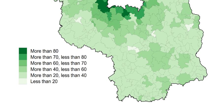
1 Introduction

Recently, the German government empowered its federal states to determine areas that
should be subject to stronger rent price regulation. We examine these two regulations
for the German state of Brandenburg. We use a regression discontinuity design (RDD)
on a dataset with actual transaction prices. We are able to identify the causal effect of
rent regulations on the sales prices of rental objects. Dwellings that are subject to the
regulations sell for 20–30 % less than they would have in the absence of regulations.

With this paper, we add to the very scarce literature on rent controls in Germany. In
comparison to the existing literature, our analysis exhibits some crucial advantages. First,
we use a unique micro dataset with official transaction prices as well as apartment char-
acteristics in Brandenburg. Second, we are able to exploit a discontinuous treatment that
allows us to employ a sharp RDD analysis. This gives us the benefit of not having to rely
on time-series data, as we believe that it is impossible to pinpoint the exact time when
expectations were being built. We base our definition of treatment and control groups on
an official report for regional housing markets in Brandenburg and measure the treatment
effect as the difference in the pooled cross section between these groups. Lastly, we focus
on sales prices. Anticipation effects in the form of rent price increases right before the in-
troduction of regulations do not pose a threat to our analysis. The effect that we measure
reflects the lowered expectation regarding future rental revenue, which is formed initially
during the introduction of the regulations.

State governments can only utilize the regulations in regions with a tight housing market.
When determining such regions, the governments need to justify their decision. Therefore,
Brandenburg commissioned a report quantifying the degree to which a region’s market
might be “tight.” The contractor translated the housing data of the municipalities into
index-score points according to a fixed scheme. Brandenburg implemented the so-called
“Kappungsgrenzenverordnung” (loosely translated: “capping limit regulation”, henceforth:
KGV) in September 2014 in 30 municipalities with scores higher than a specific threshold.
In affected municipalities, the highest possible rent increase for contracts with sitting ten-
ants was lowered from 20 % to 15 % within three years. In the exact same municipalities
and one additional region, the “Mietpreisbremse” (loosely translated: rent price brake,
henceforth: MPB) was introduced in January 2016. The regulation curtails prices of new
contracts to a maximum of 10 % above the local rent index. The quantification of a mar-
ket’s tightness that determines whether or not a regulation was implemented, provides us
with the opportunity to compare those regions that have only just been selected for regu-
lation with those that have only just not. We employ RD estimates across the regulation
treatment threshold to identify the causal price effect of these rent price controls.

These regulations pertain to the so-called second-generation rent controls, which are rather
common in industrial countries. The first generation of rent controls imposed strict rent

                                              2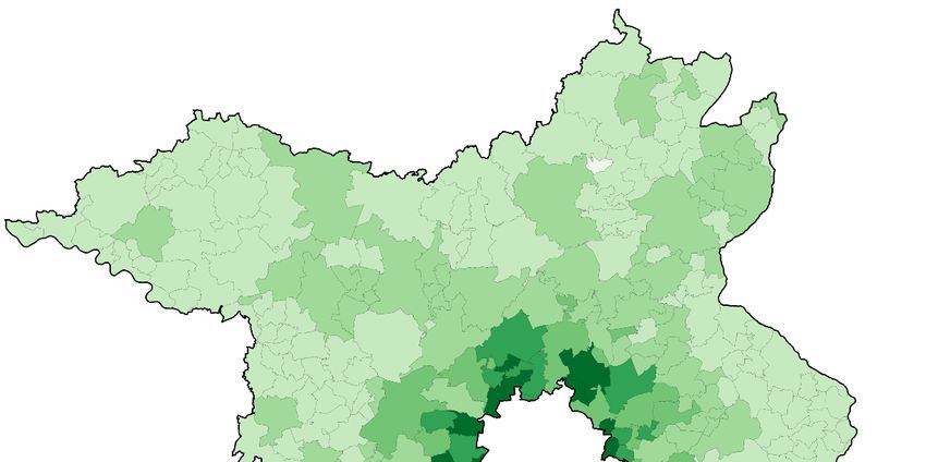
ceilings and has mostly been replaced by more flexible forms. However, scientific discussion
agrees on the negative side effects of these first-generation rent controls. They are unan-
imously regarded as an unsuitable measure to support the provision of adequate housing
at affordable costs in the long run. Even second-generation rent controls usually cause
undesired side effects. According to Arnott (1995),

      “There has been widespread agreement that rent controls discourage new con-
     struction, cause abandonment, retard maintenance, reduce mobility, generate
     mismatch between housing units and tenants, exacerbate discrimination in
     rental housing, create black markets, encourage the conversion of rental to
     owner-occupied housing, and generally short-circuit the market mechanism for
     housing.”                                                – Arnott (1995), p. 99.

Indeed, empirical studies identify a misallocation of apartments due to rent controls (see
Arnott and Igarashi, 2000; Early, 2000; Glaeser and Luttmer, 2003; Skak and Bloze, 2013).
They further observe a reduction in building activity (Glaeser and Luttmer, 2003; McFar-
lane, 2003) as well as maintenance (Olsen, 1988; Moon and Stotsky, 1993; Andersen, 1998;
Sims, 2007), and that the effect on prices only partially benefits the main target groups
(Linneman, 1987; Ault and Saba, 1990; Glaeser, 2003). In addition, even the short-run
effects on rents for regulated apartments are ambiguous. Indeed, rent controls could mit-
igate price effects that arise from rigid supply in a scenario of drastic demand shocks
(Arnott, 1995). Nagy (1997) finds a reduced rent growth for sitting tenants, but higher
asking prices for rent-controlled apartments in New York City, compared to uncontrolled
ones. Fallis and Smith (1984) and Early (2000) observe that in the Los Angeles area and
New York City, prices for uncontrolled objects rise due to rent controls in a neighboring
area. In Ontario, Smith (1988) finds rent prices for older housing units to actually be lower
due to rent controls, whereas newer apartments are more expensive.

The effects of the MPB and KGV on rents are difficult to determine at the present moment
for two reasons: First, the regulations have only been in place for a rather short period of
time. Therefore, the long-term effect of interest is overshadowed by anticipation effects.
Landlords could have set high prices prior to the regulations without being obligated to
reduce prices later. Second, the MPB is barely enforceable in its present design, since,
apart from other exceptions from the regulation, landlords do not have to reduce rents
when re-letting an apartment. They are also not obligated to share the information on the
former rent price with the new tenant. The tenant would have to rent the apartment and
then attempt to sue his landlord. This rarely happens in reality.

Nevertheless, the recently introduced rent regulation, the MPB, has already drawn a lot of
attention in media as well as in scientific discussion. Deschermeier et al. (2016) show that
prior to the introduction on rent control, a high proportion of apartments is potentially
affected in Berlin and Cologne. Thomschke and Hein (2015) conclude that at the time of
their analysis, the causal relation between regulation and rent price evolution could not yet

                                             3
be identified. However, the authors suggest that the rent control actually curtailed price
increases in Berlin. However, these early results are questioned by subsequent observations,
where prices did increase (Hein and Thomschke, 2016). In a sophisticated causal analysis
for the Berlin rental market, Thomschke (2016) estimates both the average effect on rent
prices as well as effects on the rent price distribution. He concludes that a significant rent
price effect can only be measured for the upper price segment. The second study focusing
on causal effects of the MPB is Kholodilin et al. (2016). The authors find that the MPB
does not decelerate price increases; if anything, it rather increases prices for both controlled
and uncontrolled apartments. In a recent analysis, Kholodilin et al. (2017) emphasize that
the MPB is only effective if the market rent level is sufficiently high compared to the local
rent index. They find that in those regions, the MPB is actually effective in curtailing rent
prices. In other regions, it is ineffective by design.
The situation is rather different when we look at sales prices. Even at the point of an-
nouncement, the regulations might have already posed a threat for landlords and investors.
With an unknown development of future market rents, rent regulations are likely to affect
expected returns negatively and will, therefore, decrease the value of rental objects (see
Marks, 1984; Fallis and Smith, 1984; Early and Phelps, 1999). Landlords of apartments
in rent-controlled areas presumably expected to be restricted in their price setting in the
near future. Therefore, current sales prices should already account for these future restric-
tions. Sales prices in affected regions should be lower right upon the announcement of the
implementation of rent controls. This setting allows a causal analysis even at this early
stage of being in place.
For Germany, however, Kholodilin et al. (2016) find no significant effects on sales prices.
This is quite surprising, given that intuition clearly suggests that prices are likely to
fall. The authors use asking price data and compare neighboring postal-code regions in
a difference-in-differences analysis. Their results might be distorted due to diverse price
trends of the treatment and control groups. A further distortion could stem from the
spread between asking and sales price which depends on market characteristics.1
In their new study, Kholodilin et al. (2017) find price drops at different points in time for
regulated apartments, combining a difference-in-differences estimation with a discontinuity
in time. The authors allow for three different points in time where price expectations could
have changed and find two price drops of 2.1 % and 2.7 %. However, it is impossible to
pinpoint the exact time when expectations regarding the regulations were being built.
We argue that expectations have rather spread monotonously in the time frame between
the announcement and the regulation coming into effect. Moreover, sellers might cling to
1
Han and Strange (2016) show that there are non-trivial shares of sales with transaction prices above,
below, and exactly at the list price in the USA. The size of these shares changes with the market
condition: in a boom, the portion of below-list sales drops, while at-list and above-list sales are relatively
more frequent. Henger and Voigtländer (2014) find similar results for Hamburg in Germany: the average
gap between asking and transaction price of 6.7 % changes considerably over time—from around 8 %
in 2007 and 2008 to 3.4 % in 2012. The data even indicate above-list sales for the year 2013.
4market values that were being calculated prior to the regulations. Therefore, the drop in
asking prices might be considerably less severe than for actual transaction prices. For these
reasons, we believe our findings of 20–30 % to be perfectly conceivable.
2 Institutional background
As a basic human need, housing has always been on the political agenda and has, therefore,
often been subject to regulation. For over half a century, owner occupancy was subsidized
in one way or another. The focus on ownership took a turn in 2006, when the biggest
nationwide home owner allowance (“Eigenheimzulage”) was abolished and state govern-
ments were given the power to increase real estate transfer taxes.2 In the past few years,
strong migration to cities spurred increasing rent prices. Policymakers now focus on rent
controls in order to provide affordable housing.
2.1 Brandenburg’s housing market
Brandenburg is closely related to Berlin. This is reflected in the development of building
land prices (see Figure 1). Prices in Brandenburg were relatively stable for about fifteen
years. However, in the wake of rising prices in Berlin since 2010, developed building land
in Brandenburg became more expensive as well. Prices rose by over 35 % within five years
(and this is on state average). Examining the regions surrounding Berlin in comparison
to those further away, both regions show different characteristics relevant to the housing
market.
The federal statistical office of Berlin-Brandenburg makes a distinction between the Berlin-
neighboring region and the further metropolitan area of Brandenburg.3 The former com-
prises an area of almost 3,000 square kilometers with over 900,000 inhabitants, whereas
the peripheral area is almost 27,000 square kilometers large, with more than 1.5 million
people living there. For the surrounding area of Berlin, the federal statistical office expects
population numbers to increase in the next few years, followed by a constant development
(see Figure 7 and the supplement information in the appendix as well as Amt für Statistik
Berlin-Brandenburg (Hrsg.), 2015).
Table 1 displays housing market characteristics that distinguish between regions close to
Berlin and more peripheral ones.4 As it is common in Germany, the majority of apartments
2
On the effects of the German real estate transfer taxes, see Fritzsche and Vandrei (2016), Buettner
(2017), as well as Petkova and Weichenrieder (2017).
3
This official differentiation is made since 2010 and reflects the interdependency between Berlin and its
neighboring regions in Brandenburg. The so-called further metropolitan area is therefore less struc-
turally connected to Berlin.
4
Among two other factors, these indicators were used to determine which municipalities in Brandenburg
should be subject to the KGV (see F+B, 2014). The additional indicators are the number of housing
5Figure 1: Price evolution for developed building land in Brandenburg and Berlin
220
200
180
2010 ≙ 100 160
140
120
100
80
60
1995
1996
1997
1998
1999
2000
2001
2002
2003
2004
2005
2006
2007
2008
2009
2010
2011
2012
2013
2014
2015
Brandenburg Berlin
Notes: The price decreases in recent years could be explained by increased real estate transfer
taxes. The increases were from 3.5 % to 5 % on January 1, 2011 and again to 6.5 % on June 1, 2015
in Brandenburg, and from 4.5 % to 5 % on April 1, 2012 and again to 6 % on January 1, 2014 in
Berlin (see Fritzsche and Vandrei, 2016). Data for Berlin is not available before 2008. Source: Amt
für Statistik Berlin-Brandenburg.
Table 1: Housing market indicators for Brandenburg
Indicator Berlin- Further
surrounding metropolitan
area area
Current housing demand
Share of households receiving social benefit (SGB II) 2012 8.30% 14.40%
Share of students 2012 3.20% 1.40%
Unemployment rate 2012 6.00% 10.30%
Share of long-term unemployed persons on all unemployed 33.00% 41.70%
persons 2012
Population development 2007 to 2012 4.90% -6.00%
Household development 2007 to 2012 6.30% -2.80%
Current market situation
Vacancy rate 2011 3.00% 7.30%
Share of rental apartments on all apartments 2011 53.70% 51.90%
Level of comparable rent 2013 in EUR/sqm 5.59 4.79
Level of asking rent 2013 in EUR/sqm 7.11 5.19
Development of asking rents 2007/08–2012/13 11.60% 2.30%
Spread of comparable rents and asking rents 27.30% 8.30%
Expected market situation
Population forecast to 2030 4.90% -18.50%
Share of apartments subject to rent- or tenant-control agree- 4.70% 6.80%
ments 2013–2018
Notes: The table shows housing market indicators that were used to define “tight housing markets”
in Brandenburg. Source: Own representation based on F+B (2014).
6in Brandenburg are rented out as well.5 Regions close to Berlin exhibit population growth
and a healthier labor market, thereby resulting in a higher housing demand than those
regions of the further metropolitan area of Brandenburg. This is also reflected in a tighter
housing market situation, particularly in terms of a lower vacancy rate as well as higher
rent prices. These regions also show a higher spread between asking prices and comparable
rents, thereby indicating a stronger increase in the local rent index in the near future (see
F+B, 2014).
2.2 Rent controls in Germany and Brandenburg
The high share of tenant households can partially be explained by a well-established tenant
protection in Germany, which began during the First World War. In the early 1920s, heavy
rent regulations were introduced, fixing both the rent prices for existing and new contracts.
However, after the Second World War, rent controls were gradually relaxed or abolished.
In 1972, only so-called second-generation regulations were in place, which tied price setting
to the local rent level. The nationwide capping limit was introduced in 1982, prohibiting
the increase of rents by more than 30 % within three years or above the comparable rent
level (“Mietspiegel”). A decade later, the capping limit was lowered to 20 %. Initially, this
regulation only addressed apartments with relatively high rents. In 2001, it applied to all
apartments (see Kholodilin, 2015).
In many markets, prices for current tenants were substantially lower than market prices for
new contracts, giving landlords an incentive to use eviction as a measure to increase profits.
However, there was (and still is) only a small set of reasons that legitimately justified tenant
eviction, one of which being that the landlord needs the apartment for himself or for close
relatives. Rather than looking for a new tenant, he could thus be looking for a buyer,
who would then evict the current tenants in order to claim the apartment for himself.
Although this was only possible after a waiting period of three years after converting the
rental apartment to an owner-occupied apartment, this behavior was observed in many
urban areas. This gave cause for the state government to tighten eviction laws in 1990 by
expanding the waiting period to five years. The regulation only affected areas where state
governments regarded the sufficient provision with affordable rental housing as endangered.
In 1993, this period was extended to ten years. With this tenant protection law, for the first
time, regions in Germany were discriminated based on their housing market situation.
At that time, state governments were not obliged to give any justification regarding why
they chose specific regions where the law should apply. This is also the case for the pos-
sibility to reduce the capping limit from 20 % to 15 % (KGV) in specific regions, which
allowance recipients and recipients of social benefits according to the Social Insurance Code (SGB) XII.
These indicators are only available at a district level.
5
Only 44 % of households in Germany owned their primary residence in 2014 (see Deutsche Bundesbank,
2016).
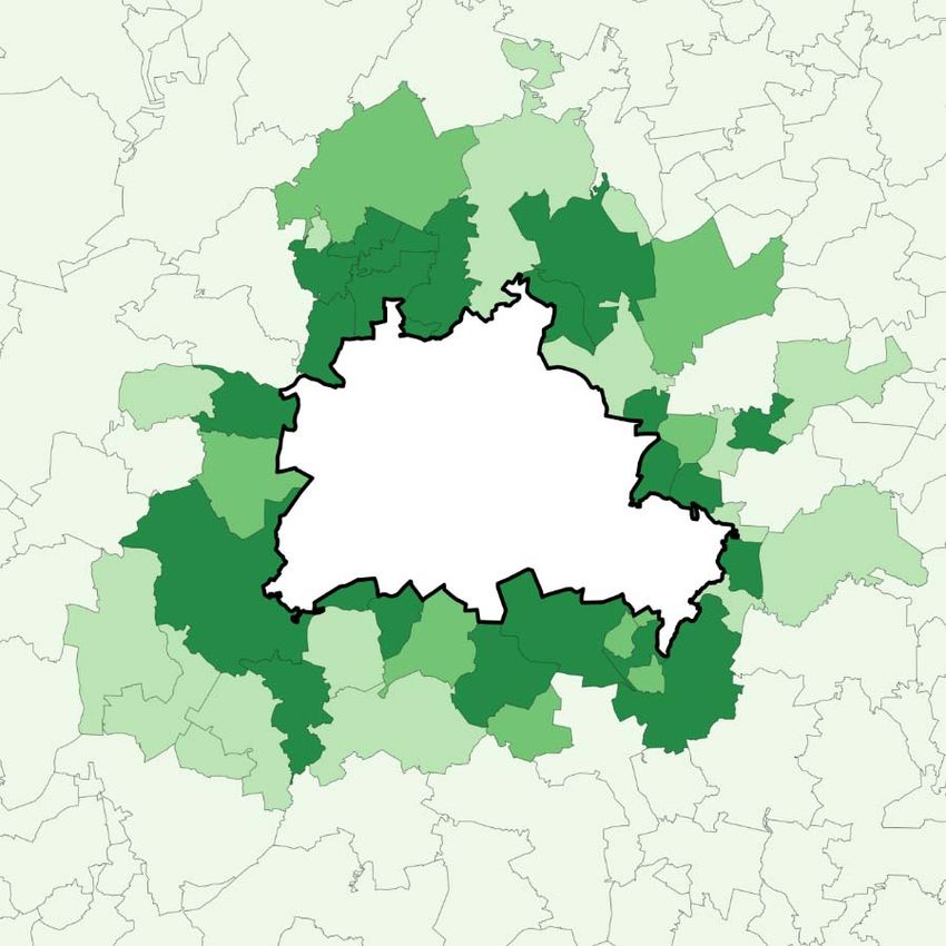
7Figure 2: Regions with lowered capping limit (KGV) and rent price regulation (MPB) in
Brandenburg
1
4 9
2 3
7 10
5 8
6
30
11 12 13
29
14
15
28 26 25 17
24 21 20
18
23 19 16
27
22
1... Oranienburg; 2… Velten, Stadt; 3… Hohen Neuendorf, Stadt;
4… Birkenwerder; 5… Heningsdorf, Stadt; 6… Glienicke/Nordbahn;
7… Mühlenbecker Land; 8…Panketal; 9… Bernau bei Berlin, Stadt;
10… Werneuchen, Stadt; 11… Hoppegarten; 12… Neuenhagen bei
Berlin; 13…Petershagen/Eggersdorf; 14… Schöneiche bei Berlin;
KGV and MPB in place 15…Erkner, Stadt; 16…Königs Wusterhausen, Stadt; 17…Eichwalde;
18… Zeuthen; 19… Wildau; 20… Schulzendorf; 21… Schönefeld;
KGV and MPB not in place
22… Rangsdorf; 23… Blankenfelde-Mahlow; 24… Großbeeren;
25… Teltow, Stadt; 26… Kleinmachnow; 27… Nuthetal;
28… Potsdam, Stadt; 29… Dallgow-Döberitz; 30… Falkensee, Stadt
Source: Own representation. Geodata: ©GeoBasis-DE / BKG 2014.
was introduced in 2013. Only with the latest rent control, prohibiting landlords to set rent
prices for new contracts that exceed the local rent level by more than 10 % (MPB), the
national government specified formal requirements. At least one of the following conditions
had to be fulfilled: (1) Rent increases considerably exceed the national average; (2) the
average rent burden6 of households considerably exceeds the national average; (3) there
is population growth without new construction covering the additional demand; (4) there
are few vacancies and a high demand.
When Brandenburg implemented the KGV in certain regions in 2014, the MPB was already
being debated upon. Only for the MPB, state governments were required to base their
decision on where to implement the regulation on housing market evidence. However,
Brandenburg already did so for the introduction of the KGV. In March 2014, Brandenburg
commissioned the external contractor F+B7 to evaluate which municipalities would exhibit
housing markets, where the provision of affordable rental housing is endangered. Among a
few other factors (see above), F+B analyzed the indicators displayed in Table 1. The values
for each indicator are then put into one of five categories, corresponding to scores of 0.00,
0.25, 0.50, 0.75, and 1. The boundaries for the lowest and highest categories represent the
extreme values for the respective indicator, while curtailing the distribution at the average
plus three standard deviations. The other categories are determined by equidistant step
lengths between these extreme values. The authors apply weights of 20 % on the current
6
The rent burden is defined as the share of a household’s gross basic rent on its disposable net income.
7
F+B Forschung und Beratung für Wohnen, Immobilien und Umwelt GmbH.
8housing demand, 75 % on the current market situation and 5 % on the expected market
situation. As a result, the authors calculate scores that can accept values between 0 and
100. The municipalities in Brandenburg range between a score of 16.0 (Steinreich) and 88.4
(Potsdam). The classification as a municipality where the sufficient provision with rental
housing under appropriate conditions is endangered corresponds to an average score plus
two standard deviations, which is 70.3 points (F+B (2014), pp. 26 ff.). This is the case for
30 municipalities in Brandenburg, which are all located in close proximity to Berlin (see
Figure 2).8 In these regions, the capping limit was lowered from 20 % to 15 %, effective
from September 1, 2014.
The very same regions in which the capping limit was lowered were subject to the MPB,
which was introduced in January 2016. Since then, a landlord was restricted in his price
setting by two regulations: First, due to the KGV, he could only raise prices for current
tenants for a maximum of 15 % within three years.9 Second, with the MPB, new tenants
could not be charged a price that exceeds the local rent level by more than 10 %.10
3 Conceptual framework
Both price regulations are linked to the local rent index, but in different ways. The MPB
restricts landlords from asking for rents that are more than ten percent above the local
rent index. Therefore, a low index goes along with a stronger restriction. However, the
KGV is only binding if the local rent level is over 15 % higher than the current rent that
a tenant pays his landlord. In this case, a landlord could only raise the rent by 15 % and
not by a maximum of 20 % within three years, as would be the case without the KGV.
Mostly, the KGV is relevant for cases where the landlord did not raise the rent for a long
period of time. This can particularly be the case if he has had a price-binding agreement
as part of a social housing program.11 After the price-binding period, the local rent index
will probably be above the rent he currently charges and the KGV might be binding.
The MPB is presumably the regulation with the higher impact for the residential housing
market. We illustrate this in the following model:
8
Approximately half of Brandenburg’s municipalities received scores from 30 to 40 points. Over 50 points
are quite equally represented and can particularly be found in the Berlin-surrounding area (see also
Figure 4 in Section 5.1).
9
Presumably, for many cases, this regulation is ineffective. Even without the lowered capping limit, the
price increase is restricted to the local rent level. There are some exceptions that allow a landlord to
raise the rent for a current tenant above the local rent index: If he conducted modernizations, he can
raise the yearly rent by 11 % of the incurred costs. Moreover, the KGV does not apply for graduated
rental agreements, where price increases are agreed upon within the rental contract. The same applies
for index-linked rents which are connected to the consumer price index.
10
Apartments built or extensively reconstructed after January 1, 2014 as well as furnished apartments are
exemptions. Moreover, the landlord is not obliged to reduce the rent price he received from the previous
tenants.
11
In such a program, the landlord usually receives subsidies in the form of a cheap loan or a monthly
grant. The rent is often fixed for over ten years.
9Potential investors are willing to pay the present value of the expected rental income for
the remaining useful life of L years for an apartment:12
L
X
P Vt = pt , (1)
t=1
where pt is the yearly (net) rental income the investor/landlord receives in year t. He
expects the market rent to increase by a yearly rate of r. Furthermore, he expects a tenant
to rent the apartment for a time of C years. pt depends on whether the landlord forms a
contract with (a) a new tenant or (b) already has a tenant and can just decide to raise
the current rent. (
pat if t = 1 + nC, ∀n ∈ N
pt = , (2)
pbt else
with
pat = min {pm
t , 1.1It } ,
(3)
pm m
t = (1 + r)pt−1 ,
and
pbt = max {pt−1 , min{1.15pt−3 , It }} .
pat is therefore only charged in the first period with a new tenant. This is the case every
C years. With the MPB in place, pat is either the market rent, pm
t , or the local rent index,
It , plus ten percent. In all other periods, the landlord can only increase the rent for his
current tenant if It is higher than his current price. In this case, he can increase his current
rent by a maximum of 15 % in relation to the price he charged three years ago, due to the
KGV. However, the new rent must not exceed the rent index.
The rent index is the arithmetic mean of newly agreed upon rents as well as changes in
existing contracts over the last four years. We assume a constant market-price growth rate
and further assume that the number of new contracts in each period is constant. Since the
rent index is calculated with prices of previous periods, it is always lower than the current
market rent (due to positive growth). For this reason, a landlord who just agreed upon a
contract with a new tenant, cannot raise the rent in the following few years.13 From the
moment the rent index surpasses the current rent price, a rational landlord would increase
the rent for a sitting tenant for every following year. These increases, in turn, are also
considered in the local rent indices in the following four years. Therefore, the local rent
index is indirectly influenced by market prices from even more than four years ago.
To illustrate, we compare two apartments, of which one is subject to the regulations and
the other is not. We assume C = 10, L = 20, an exogenously given market price, pm
1 , of
12
For facilitation, we disregard maintenance costs, transaction costs, search costs, search duration, interest
rates, and time preferences and we assume risk neutrality. Policymakers are aware of potential side
effects due to the reforms. For example, rent price increases due to specific maintenance activities are
therefore exempt from the regulations.
13
Therefore, the KGV would not be binding.
10Figure 3: Simulation of regulated and unregulated asking prices.
U U
3ULFHLQ(85VTP
3ULFHLQ(85VTP
3HULRG 3HULRG
8QUHJXODWHG 5HJXODWHG 8QUHJXODWHG 5HJXODWHG
U U
3ULFHLQ(85VTP
3ULFHLQ(85VTP
3HULRG 3HULRG
8QUHJXODWHG 5HJXODWHG 8QUHJXODWHG 5HJXODWHG
Notes: Simulation results for regulated and unregulated market rents. The MPB and the KGV are
introduced after period 5. The KGV is not binding. Source: Own representation.
€ 5.00 with an annual growth of r = 3 %. Even without the new regulations, the rent for
sitting tenants cannot be increased above the rent index. Initially, landlords will charge
the market rent. For the given parameters, they will not be able to raise prices due to a
lower rent index for the following five years. Thereafter, they increase prices to meet the
index for the remaining four years that the tenant is present. Given that the number of
contracts per year is constant, ten percent of the apartments get new tenants with new
prices, whereas 40 % of the apartments become more expensive for sitting tenants (and in
40 % of the apartments, prices remain unchanged). Therefore, new contracts only have a
weight of 20 % in the local rent index and prices for existing contracts have 80 %.14 The
market price with these parameters is 17.03 % higher, without the regulations.
Figure 3 shows that the gap between the unregulated and regulated asking price increases
in the rent’s growth rate. For the abovementioned case of 3 % growth, the unregulated
market rent would be € 10.16 per square meter. With the MPB in place, € 7.77 would
be the highest legitimate asking price. This is reflected in the landlord’s present value. If
he invested at the beginning of period 6, the regulation would lower his present value by
11.8 %. If he expected prices to grow by less than 1.8 % per year, the regulation would
not be binding. He expects to lose 20.3 % at r = 4 % and 28.0 % at r = 5 % due to the
regulation.
14
Note that these populations and the local rent index are interdependent and the mentioned sizes are at
equilibrium.
114 Data
Fortunately, we are able to rely on a complete survey of micro data with actual transaction
prices provided by the Superior Property Valuation Committee of Brandenburg. There are
sixteen county-level Property Valuation Committees in Brandenburg that receive copies
of every sales contract for real estate transactions that are conducted in the respective
administrative area. Therefore the committees hold information on the transaction price,
the exact location of the real estate, as well as the date the contract was finalized. Through
surveys, the committees collect data on the estates’ characteristics, such as living space,
year of construction, number of housing units in the building, or even the shape of the
roof. In addition, they enrich the data with information regarding the location, includ-
ing a calculated land value. The Superior Property Valuation Committee collects and
administrates the data at the state level.
Table 2 displays the summary statistics for the main variables of our data. The sample
covers all apartment sales between January 2011 and August 2017. Altogether, the data
comprise 11,111 individual sales that include information on the living space. Approxi-
mately a third of the transactions are first sales, that is, they were not occupied prior to
being sold and would thus not be subject to the MPB. For the majority of the transacted
apartments, we have information on the renting situation. Unfortunately, the rent price
is only known for about 2,000 observations. However, we know that at the time of sale,
approximately half of the apartments came with an active rental contract.
The average values for living space and the number of rooms for the transacted apartments
in our data are smaller than the average values of the census on buildings and houses in
2011: 84 square meters living space and 4.2 rooms. This reflects the fact that, first, apart-
ments are usually smaller than single- and two-family houses. Second, smaller housings are
overrepresented in transaction data compared to stock data, as they tend to be transacted
more frequently. The age variable corresponds to the year of construction or to the year
of constructional changes to the apartment. Therefore, it indicates the remaining period
of use. In about 475 cases, construction was only completed the next year, or in the year
after in a few cases. On average, an apartment in our dataset is situated in a house with
a total of 26 units. This stems from the fact that, again, we only regard apartments that
are not in single- or two-family houses.
The land value (German: Bodenrichtwert) represents the monetary per square-meter value
of a building lot, apart from any structures that might be on that lot. The Property Val-
uation Committees calculate land values for a group of lots with similar characteristics.
Therefore, these land-value zones allow for far finer analyses than the municipality level.
However, there are still differences in actual land values within the land-value zones. The
micro-location quality provides additional information. The variable considers character-
12Table 2: Descriptive statistics
Variable Obs Mean Std. Dev. Min Max
General
Sales price (EUR/sqm) 11,111 1,844.83 1,011.26 43 8,201
First sale (dummy) 11,111 0.32 0.47 0 1
Let (dummy) 8,395 0.49 0.50 0 1
Rent price (EUR/sqm) 2,034 6.77 1.96 0 18
Property characteristics
Living space (sqm) 11,111 78.32 31.55 17 917
Number of bedrooms 8,402 2.79 1.01 1 24
Age (years) 11,111 12.43 11.76 -2* 236
Number of units 7,613 25.56 32.29 1 524
Location characteristics
Land value 10,757 139.95 108.33 0 650
Location quality (1–9) 6,342 5.83 1.18 2 9
No special location (dummy) 8,845 0.64 0.48 0 1
Near water (dummy) 8,845 0.11 0.31 0 1
Second row (dummy) 8,845 0.25 0.43 0 1
Noisy or near landfill (dummy) 8,845 0.01 0.08 0 1
Municipality score 11,111 74.06 15.67 22 88
Notes: * The age of an apartment represents the time difference of the finalization of the sales
contract and the year of construction or, if applicable, the year of constructional changes. A negative
age indicates that an apartment is sold prior to constructions being completed.
istics that explicitly influence the land value within a land-value zone. Examples of such
characteristics are close proximity to water or being exposed to noise.
In addition to the data provided by the Superior Property Valuation Committee in Bran-
denburg, we allocate municipality-scores, calculated in F+B (2014), to each transaction.
High scores indicate a so-called tightness of a housing market in the sense that a high de-
mand for rental housing might not be met at affordable prices. Municipalities in Berlin’s
neighboring areas and/or with a good infrastructural connection typically show higher
scores. Both are true for the capital and largest city of Brandenburg, Potsdam, which has
the highest score of 88.4 points. Overall, 169 of a total 418 municipalities are represented in
the data. In particular small municipalities and those with a higher share of single-family
homes are less likely to host an apartment transaction during the regarded time frame.
This is also the case for the lowest-scoring municipalities: Steinreich (16.0), Drahnsdorf
(20.0), and Heideblick (20.5). However, all municipalities with a score greater than 60 are
included in the data.
In the following analysis, we exclude first sales, as these are most likely not subject to
the reforms. We also exclude the municipality of Ahrensfelde, since it constitutes the one
exception of being subject to the MPB, but not to the KGV.15 We have a few cases in the
15
While the KGV was not introduced due to a score of 67.9, Brandenburg decided to introduce the MPB,
13data, where entire houses and therefore multiple apartments are transacted simultaneously.
Treating entire house sales as multiple observations of apartment sales would distort our
data. To prevent this, we compute these cases as single apartment transactions, using the
mean apartment price and characteristics.16
5 Empirical analysis
5.1 Identification strategy
We test whether rent price regulation has an impact on transaction prices of affected
apartments. To identify this effect, we employ a regression discontinuity approach (see
Thistlethwaite and Campbell, 1960; Hahn et al., 2001; Imbens and Lemieux, 2008; Lee
and Lemieux, 2010). The basic idea is that around the treatment threshold (70.3 points),
municipalities are so similar in those characteristics that determine whether or not they
receive the treatment, that the actual assignment can be regarded as being random. Since
the apartments in those municipalities are unalterably located there, they also receive
treatment randomly. Therefore, in the best-case scenario, these apartments show the same
characteristics on average, with the only difference being whether or not they are subject
to rent regulations. With this design, we are able to estimate the causal price effect of the
rent regulations on those apartments.
Figure 4 depicts the regional distribution of the municipality scores calculated in F+B
(2014). The right-hand side illustrates the control and treatment groups within a band-
width of five score points to either side of the cutoff point of 70.3, above which the treat-
ment is given. In many cases, treated regions are neighboring non-treated ones. Since score
levels reflect the local housing market, in the absence of regulations, investors who would
have invested in a market slightly above the cutoff point, might now have an incentive to
select a neighboring location with a slightly lower score. In this regard, our estimation can
be considered optimistic. The coefficients that we find might partially be driven not only
by lower prices in treated municipalities, but also by higher prices due to spillover effects
to non-treated ones. The data we use for the calculations include the living space, age,
land value, and the transaction date of the apartments. Further control variables would
either restrict our sample size too heavily, as we do not have this information for all obser-
vations (e. g. the “let” dummy variable), or are strongly correlated with other covariates
(e. g. number of rooms with living space). The sample we use comprises 6,303 observations
for the entire time frame.
since demand picked up rapidly in the recent past.
16
As a robustness check, we exclude all sales, where multiple apartments of the same house were transacted
simultaneously (see Section 6.2).
14Figure 4: Municipality score distribution in Brandenburg (left) and assignment to treat-
ment and control groups (right)
Over 75.3
Over 70.3, below 75.3
Over 65.3, below 70.3
Below 65.3
Over 80 Treatment group: Werneuchen, Wildau, Oranienburg,
Eichwalde, Dallgow-Döberitz, Rangsdorf, Neuenhagen bei Berlin,
Over 70, below 80 Schulzendorf, Großbeeren
Over 60, below 70
Over 40, below 60 Control group: Strausberg, Rüdnitz, Ludwigsfelde,
Over 20, below 40 Grünheide/Mark, Seddiner See, Woltersdorf, Michendorf,
Below 20 Ahrensfelde, Wandlitz, Werder (Havel), Stahnsdorf,
Leegebruch, Gosen-Neu Zittau, Schwielowsee,
Fredersdorf-Vogelsdorf, Brieselang
Data: F+B (2014). Geodata: ©GeoBasis-DE / BKG 2014. Notes: The assignment to treatment and
control groups is based on a bandwidth of five score points above and below the cutoff of 70.3
points.
We define the treatment as receiving both the KGV and the MPB. Therefore, our calcu-
lations are more optimistic in comparison with Kholodilin et al. (2017), who concentrate
on the MPB. The treatment is assigned to all municipalities with a score higher than
70.3 points. All regions below that threshold are untreated. Therefore, we have a sharp
discontinuity at the cutoff. To identify a causal effect, we must ensure that there is no
additional discontinuity at the cutoff that would confound our interpretation. This is not
the case since the municipality scores were used for the sole purpose of identifying regions
that should receive rent regulation. Therefore, the cutoff has no further meaning other
than allocating the treatment. We conclude that there is no discontinuity in potential
outcomes.
Further, we need to check whether there might be manipulation into treatment or non-
treatment. Observations of our sample might have influenced their score in order to receive
or to be exempt from rent price regulations. Our data comprise single transactions, whose
assigned score depends solely on the municipality they are located in. If at all existent, the
influence of one single apartment (respectively of its owner) on the municipality’s score
is vanishingly small. Thus, the concern of manipulation does not lie on the level of single
observations but rather on the level of the corresponding municipalities. The strongest
argument against manipulation on this level is that the scores are based on a report that
utilizes actual housing market data. Moreover, it was commissioned not by the local but the
state government. Thus, it does not seem plausible that a municipality was able to actively
15influence, for example, its vacancy rate in order to lower (or increase) its score. Further,
the cutoff point itself appears to not be politically influenced, since it is fixed at exactly
the distribution’s mean value plus two standard deviations. However, the report by F+B
(2014) includes a municipality survey that might raise concern regarding manipulation.
Ultimately, the survey was not used to calculate the municipality scores. We do not know
for sure, though, that the indicator weights that were used are free from manipulation.
To tackle this issue, we conduct a density test and find no significant bunching of scores
around the cutoff point of 70.3 (see Table 10 and Figure 8 in the appendix for details).
To further exclude the possibility of manipulation, the covariates need to be balanced
around the threshold. This is most certainly the case for the apartments’ age as well as
the date the transactions took place (see Figure 9 in the appendix). Moreover, the living
space appears rather continuous; however, land values suggest a discontinuity at the cutoff.
This does raise a concern regarding whether transactions are indeed distributed randomly.
Examining the earlier time frame, though, we can see that the distribution in land values
was balanced before the treatment. This gives reason to believe that the current land
values already, at least partly, reflect the negative impact of regulation on property prices.
Since the committees of evaluation experts calculate land values on a yearly basis, this
is indeed possible. Therefore, we conduct our regression analysis both with and without
inclusion of land values.
The time frame in our data spans from 2011 to 2017. In Brandenburg, the KGV came
into effect in September 2014 and the MPB in January 2016. Since media coverage on
the topic was very strong, it seems plausible that potential investors were aware of the
regulations by January 2016.17 It makes sense to also examine a time frame where there had
been no treatment. The treatment in our context is that investors know of the rent price
regulation that might affect future rental income. Although both instruments were already
discussed even before 2014, it remained unclear, which regions, if any, would be subject to
the regulation. If investors anticipated the introduction of a rent price regulation in any
of Brandenburg’s regions, their expectations should have been similar for those regions
around the cutoff point. For this reason, we can span our pre-treatment time frame to
April 2014, since the technical report evaluating the municipalities’ housing markets was
not published before May 2014. Therefore, the pre-treatment period stretches from January
2011 to April 2014, while the post-treatment period is from January 2016 to November
2017.18
In our baseline regression, we estimate the local average treatment effect in a pooled
17
The KGV is generally less known compared to the MPB. However, for our analysis, it is more important
that the information distribution did not change in the regarded time frame, rather than everybody
being fully informed.
18
Potentially, changes in real estate transfer taxes could have had a great impact on apartment prices
during this time. However, Brandenburg raised transfer taxes on two occasions: in January 2011 and
in July 2015. Therefore, transfer taxes were constant within the pre- and post-treatment time frame,
respectively.
16cross-section RD approach. We use a local polynomial to smooth the functional form
of the underlying relationship between sales price and the municipality score. Since this
relationship might be stronger for very high and very low values of the municipality score,
we conduct the estimation with a quadratic smoothing function. Our baseline regression
function takes the following form:
pi = α + β1 Ti
+ β2 (xi − xc ) + β3 (xi − xc )2 + β4 Ti (xi − xc ) + β5 Ti (xi − xc )2 (4)
+ δXi0 + i .
pi denotes the log sales price of an apartment i. The coefficient of interest is β1 , which
measures the treatment effect around the threshold. Ti is a dummy variable that equals
one if a transaction takes place in a treated municipality and zero otherwise. xi represents
the position on the running variable, whereas xc is fixed at the cutoff of 70.3. Thus, the
difference indicates the municipality score distance to the threshold. This difference and
the squared difference control for the smooth function of the relationship between running
and the outcome variable, which we assume to be quadratic at this point.19 We also
include an interaction term of the score distance with the treatment dummy to allow for
different reactions of treated and non-treated units to the treatment. In the regression,
we use a triangular kernel function. Hereby, observations that are closer to the threshold
receive greater weights. Xi depicts a vector of control variables, such as living space and
the apartment’s age, with its corresponding coefficients δ. α is the intercept and i is the
standard error, clustered for municipalities.
5.2 Results
Figure 5 illustrates the discontinuity of prices per square meter at the threshold of 70.3
score points. The first thing to notice is that for the entire range of the sample, the
relationship appears to be rather linear and continuous, both for the pre- and the after-
treatment period (Figure 5 plots 1a and 1b). Further, for the effect around the threshold,
prices are quite clearly continuous for the pooled cross section from 2011 to 2014 (plot 2a
and 3a). However, in the time frame after the treatment, observations that are located in
municipalities with scores just slightly above the cutoff do indeed appear to sell for smaller
prices, as plots 2b and 3b suggest. This significance of this effect is illustrated by the fact
that the 95 % confidence intervals of the close-to-cutoff observations do not overlap—in
contrast to the pre-treatment period. This result does not change when we add control
variables.
Table 3 displays the baseline regression results. In a nutshell, we find that the rent reg-
ulations reduce sales prices by approximately 27 %. The first three columns show that in
19
In section 6.3, we also use polynomial orders 0, 1, and 3 for the (interacted) smoothing function.
17Figure 5: Distribution of mean prices per square meter for municipality scores
1a) Pre treatment, full sample, linear 1b) Post treatment, full sample, linear
250
250
200
200
Sales price in 1000 EUR
Sales price in 1000 EUR
150
150
100
100
50
50
0
0
20 40 60 80 100 20 40 60 80 100
Municipality score Municipality score
Sample average within bin Polynomial fit of order 1 Sample average within bin Polynomial fit of order 1
2a) Pre treatment, around cutoff, linear 2b) Post treatment, around cutoff, linear
250
250 200
200
Sales price in 1000 EUR
Sales price in 1000 EUR
150
150
100
100
50
50
0
0
60 65 70 75 80 60 65 70 75 80
Municipality score Municipality score
Sample average within bin Polynomial fit of order 1 Sample average within bin Polynomial fit of order 1
3a) Pre treatment, around cutoff, quadratic 3b) Post treatment, around cutoff, quadratic
250
250
200
200
Sales price in 1000 EUR
Sales price in 1000 EUR
150
150
100
100
50
50
0
0
60 65 70 75 80 60 65 70 75 80
Municipality score Municipality score
Sample average within bin Polynomial fit of order 2 Sample average within bin Polynomial fit of order 2
Notes: The graphs show the municipality mean prices per square meter for municipality scores
before (left) and after (right) the treatment for the entire sample (top) and around the treatment
cutoff of 70.3 points (bottom). The mid and bottom figures display 95 % confidence intervals with
standard errors clustered at municipality level. The vertical lines indicates the cutoff at 70.3 points,
above which the treatment is given. The other lines show the best weighted least-squares fit of a
first- (top and mid) and second- (bottom) order polynomial. The pre-treatment time frame is
January 2011 to April 2014; the post-treatment time frame is January 2016 to November 2017.
The displayed bins are calculated to be evenly spaced and to mimic the variance of the raw data
(see Cattaneo et al. (2017a) for details).
18Table 3: Baseline results
Dependent variable: sales price (logged)
Time frame Pre-treatment Post-treatment
RDD estimator
Coefficient -0.207 -0.048 0.092 0.055 -0.565*** -0.259 -0.293* -0.269**
Std. error 0.192 0.178 0.153 0.122 0.193 0.171 0.154 0.133
p-value 0.281 0.788 0.549 0.653 0.003 0.130 0.056 0.043
Control variables
Living space NO YES YES YES NO YES YES YES
Living space squared NO NO YES YES NO NO YES YES
Age NO NO YES YES NO NO YES YES
Age squared NO NO YES YES NO NO YES YES
Land value NO NO NO YES NO NO NO YES
Date NO NO YES YES NO NO YES YES
Obs. 419 419 419 417 366 366 366 364
Obs.– 262 262 262 260 242 242 242 241
Obs.+ 157 157 157 157 124 124 124 123
Notes: Significance levels: *** 0.01, ** 0.05, and * 0.10. Standard errors are clustered at municipality
level. Pre-treatment time frame: January 2011 to April 2014; post-treatment time frame: January
2016 to November 2017. Quadratic smoothing function. Bandwidth: 5 points to either side of the
cutoff of 70.3. Kernel type: triangular. Obs.– (obs.+) denotes the number of observations below
(above) the cutoff within the respective bandwidth.
the pre-treatment period, between January 2011 and April 2014, the RDD estimator is
insignificant. When controlling for the living space, the smaller standard errors give us
confidence that the true coefficient is in fact close to zero. Put simply, we do not find a
treatment effect when there was no treatment. This is the case for both regressing with
just the living space as a control variable as well as other controls, such as the age of an
apartment and its land value. We also include the date variable to account for a supposedly
linear trend of increasing prices. For the post-treatment frame, the effect is considerably
larger. Simply regressing on the sales price overestimates the effect, since the treatment
group shows lower prices even in the pre-treatment frame, when not controlling for any
covariates. Adding the living space as the only control variable does not reduce the vari-
ance by much. However, it does reduce the coefficient to a level that does not differ from
zero at a significant level. The last column is the most interesting one. Adding further
controls, such as the age, land value, and the date of transaction, the coefficient remains
unchanged, but gains significance at the 5 % level. Apartments that are similar in terms
of living space, age, land value, and the transaction date, realize sales prices that are
significantly lower if the apartment is located in a municipality that only just received
treatment. On average, such an apartment sells for a price of approximately 27 % below
an object that is not treated.
As suggested earlier, our estimation can be regarded as optimistic. The external validity
of our results could be limited due to the fact that we cannot exclude spillover effects
to neighboring municipalities. Therefore, it could be possible that owners in unregulated
19municipalities even profit from the regulations in the form of price increases. Thus, the
effect that we find addresses the price effect differences between treated and non-treated
apartments, which might have higher prices due to the regulations. When regarding the
scenario of no introduction of any treatment at all as the counterfactual world to our
setting, we expect the coefficients to be slightly lower. In most cases, the introduction of
the regarded regulations will always evoke spillover effects, since treated municipalities
are almost always neighboring non-treated ones. Moreover, municipalities are typically
fairly small. For this reason, we expect spillovers not only at the edges of a municipality.
Particularly for investors, choosing the neighboring municipality will not be much of a
problem.
However, the results above show lower sales prices of almost 30 % when we factor in that the
land value also decreases. Taking possible spillovers and the following sensitivity analyses
into account, we are confident that the effect of the regarded rent price regulations on
sales prices is in the range of 20 % to 30 %.20 In comparison with the study by Kholodilin
et al. (2017), our findings suggest much greater effects of rent price regulation on sales
prices. This can be explained by the fact that, first, we do assume a sharp treatment
timing. The reforms should affect market prices when people are aware of the reforms.
The proportion of informed market participants does not switch from zero to one from
one day to the next. Rather, information spreads monotonously over time. Therefore, the
effect we find does not only include the 2.1 % and the 2.7 % drop in prices that Kholodilin
et al. (2017) found. It also includes the (presumably smaller, but many) price drops at
other dates between announcement and introduction of the reforms. Second, we measure
not only the MPB but also the KGV. The latter is arguably not binding (see Section 3).
However, if it has any effect on prices, it is in the same direction as the MPB. Third, we
use transaction data rather than asking prices. Therefore, our effect does not only include
lowered price expectations by sellers but also a discouragement of investors. We argue
that it is primarily potential buyers who drive down the price due to market restrictions.
Owners, however, might orient asking prices on past sales or price assessments that took
place before the regulations were announced.
6 Robustness exercises
In this section, we conduct a number of robustness exercises to check the sensitivity of the
measured treatment effect toward different model specifications.
20
Section 6.5 suggests that sales prices below the cutoff are decreasing compared to apartments in munic-
ipalities with even lower scores. Therefore, the difference that we measure in the baseline regression is
dominantly driven by comparably decreasing prices in the treatment group.
206.1 Clusters
When we look at the map on the right-hand side of Figure 4, we might be concerned that
the distribution of control and treatment observations is geographically clustered. Indeed,
there are four municipalities southwest of Berlin that are not neighboring Berlin and that
all belong to the control group. In addition, they are all located in the county Potsdam-
Mittelmark. Figure 6 shows that the observations in this county constitute more than a
third of all observations used in the baseline regression. The concern is that there might
be a price trend in the cluster that does not show in the other areas we examine. More
specifically, our main coefficient might be driven not by an actual drop in prices of treated
observations but rather by price increases of non-treated ones (in the cluster). To test for
this, we conduct the same exercise as we did for the baseline regression, while omitting
the data of Potsdam-Mittelmark.
The results are displayed in Table 4. Compared to the baseline results in Section 5.2, we
lose 127 observations in our treatment group. This provides us with an almost perfectly
balanced sample. The results support our previous findings. What is worth noticing is
that the treatment effect of 25 % is significant at the highest significance level, while the
effect is measured at almost exactly zero for the period prior to treatment. This gives us
confidence that our baseline results are not driven by geographical clusters.
Figure 6: Distribution of observations in the treatment and control groups by county
40%
35%
Share of observations
30%
25%
20%
15%
10%
5%
0%
12069 12072 12064 12063 12065 12060 12061 12067
County (5-digit code)
Control group Treatment group
Notes: The figure shows the distribution of observations in the post-treatment time frame (January
2016 to November 2017). The treatment (control) group includes observations with municipality
scores from 70.3 to 75.3 (65.3 to 70.3) points. The represented counties include: 12069 Potsdam-
Mittelmark, 12072 Teltow-Fläming, 12064 Märkisch-Oderland, 12063 Havelland, 12065 Oberhavel,
12060 Barnim, 12061 Dahme-Spreewald, and 12067 Oder-Spree.
21You can also read