Information, incentives, and goals in election forecasts

Judgment and Decision Making, Vol. 15, No. 5, September 2020, pp. 863–880

 Information, incentives, and goals in election forecasts

 Andrew Gelman∗ Jessica Hullman† Christopher Wlezien‡ George Elliott Morris§

 Abstract

 Presidential elections can be forecast using information from political and economic conditions, polls, and a statistical model
 of changes in public opinion over time. However, these “knowns” about how to make a good presidential election forecast come
 with many unknowns due to the challenges of evaluating forecast calibration and communication. We highlight how incentives
 may shape forecasts, and particularly forecast uncertainty, in light of calibration challenges. We illustrate these challenges in
 creating, communicating, and evaluating election predictions, using the Economist and Fivethirtyeight forecasts of the 2020
 election as examples, and offer recommendations for forecasters and scholars.
 Keywords: forecasting, elections, polls, probability

1 What we know about forecasting Although these referendum judgments are important for
 presidential elections, political ideology also matters. Can-
 presidential elections didates gain votes by moving toward the median voter (Erik-
 son, MacKuen & Stimson, 2002), and partisanship can in-
We describe key components of a presidential election fore-
 fluence the impact of economics and other short-term forces
cast based on lessons learned from research and practice.
 (Kayser and Wlezien, 2011, Abramowitz, 2012). As the
 campaign progresses, various fundamentals of an election
 increasingly become reflected in — and evident from — the
1.1 Political and economic fundamentals
 polls (Wlezien and Erikson, 2004, Erikson and Wlezien,
There is a large literature in political science and economics 2012).
about factors that predict election outcomes; notable con- These general ideas are hardly new; for example, a promi-
tributions include Fair (1978), Fiorina (1981), Rosenstone nent sports oddsmaker described how he handicapped pres-
(1983), Holbrook (1991), Campbell (1992), Lewis-Beck and idential elections in 1948 and 1972 based on the relative
Rice (1992), Wlezien and Erikson (1996) & Hibbs (2000). strengths and weaknesses of the candidates (Snyder, 1975).
That research finds that the incumbent party candidate typ- But one value of a formal academic approach to forecasting
ically does better in times of strong economic growth, high is that it can better allow integration of data from multiple
presidential approval ratings & when the party is not seek- sources, by systematically using information that appear to
ing a third consecutive term. This latter may reflect a “cost have been predictive in the past. In addition, understanding
of ruling” effect, where governing parties tend to lose vote the successes and failures of formal forecasting methods can
share the longer they are in power, which has been shown inform theories about public opinion and voting behavior.
to impact elections around the world (Paldam, 1986, Cuzan, With the increase in political polarization in recent
2015). decades (Abramowitz, 2010, Fiorina, 2017), there is also
 reason to believe that elections should be both more and less
 predictable than in the past: more predictable in the sense
 We thank Joshua Goldstein, Merlin Heidemanns, Dhruv Madeka, Yair that voters are less subject to election-specific influences as
Ghitza, Annie Liang, Doug Rivers, Bob Erikson, Bob Shapiro, Jon Baron,
and the anonymous reviewers for helpful comments, and the National Sci-
 they will just vote their party anyway, and less predictable in
ence Foundation, Institute of Education Sciences, Office of Naval Research, that, elections should be closer to evenly balanced contests.
National Institutes of Health, Sloan Foundation, and Schmidt Futures for The latter can be seen from recent election outcomes them-
financial support.
 Copyright: © 2020. The authors license this article under the terms of
 selves, both presidential and congressional. To put it another
the Creative Commons Attribution 3.0 License. way, a given uncertainty in the predicted vote share for the
 ∗ Department of Statistics and Department of Political Science, Columbia
 two parties corresponds to a much greater uncertainty in the
University, New York. Email: gelman@stat.columbia.edu.
 † Department of Computer Science & Engineering and Medill School of election outcome if the forecast vote share is 50/50 than if it
Journalism, Northwestern University. is 55/45, as small shifts matter more in the former than the
 ‡ Department of Government, University of Texas at Austin.
 latter.
 § The Economist.

 863

Judgment and Decision Making, Vol. 15, No. 5, September 2020 Information, incentives, and goals in election forecasts 864

1.2 Pre-election surveys and poll aggregation A single survey yields an estimate and standard error
 which is often interpreted as a probabilistic snapshot or fore-
Election campaigns have, we assume, canvassed potential cast of public opinion: for example, an estimate of 53%±2%
voters for as long as there have been elections, and the Gallup would correspond to an approximate 95% predictive interval
poll in the 1930s propagated general awareness that it is of (49%, 57%) for a candidate’s support in the population.
possible to learn about national public opinion from surveys. This Bayesian interpretation of a classical confidence inter-
Indeed, even the much-maligned Literary Digest poll of 1936 val is correct only in the context of a (generally inappropri-
would not have performed so badly had it been adjusted ate) uniform prior. With poll aggregation, however, there
for demographics in the manner of modern polling (Lohr is an implicit or explicit time series model which, in effect,
& Brick, 2017). The ubiquity of polling has changed the serves as a prior for the analysis of any given poll. Thus,
relationship between government and voters, which George poll aggregation should be able to produce a probabilistic
Gallup and others have argued is good for democracy (Igo, “nowcast” of current vote preferences and give a sense of
2006), while others have offered more sinister visions of the uncertainty in opinion at any given time, evolving during
voter manipulation (Burdick, 1964). the campaign, as the polls become increasingly informative
 In any case, polling has moved from in-person interviews about the fundamentals.
to telephone calls and then in many cases to the internet, fol-
lowing sharp declines in response rates and increases in costs
of high-quality telephone polls. Now we are overwhelmed 1.3 State and national predictions
with state and national polls during every election season, Political science forecasting of U.S. presidential elections
with an expectation of a new sounding of public opinion has traditionally focused on the popular vote, not the elec-
within days of every major news event. toral college result. This allows us to estimate the national
 With the proliferation of polls have come aggregators such forces at work, what sometimes is referred to among elec-
as Real Clear Politics, which report the latest polls along toral scholars as the "swing" between elections. But national
with smoothed averages for national and state races. Polls vote predictions actually are forecasts of the candidates’ vote
thus supply ever more raw material for pundits, but this is shares in the states and the District of Columbia; thus, we
happening in a politically polarized environment in which are talking about forecasting a vector of length 51 (plus extra
campaign polls are more stable than every before, and even jurisdictions from the congressional districts in Maine and
much of the relatively small swings that do appear can be Nebraska), and state-by-state forecasts are important unto
attributed to differential nonresponse (Gelman, Goel, et al., themselves given that the electoral college actually chooses
2016). the president. This was explicitly addressed in early fore-
 Surveys are not perfect, and a recent study of U.S. pres- casting efforts, including those of Rosenstone (1983) and
idential, senatorial, and gubernatorial races found that state Campbell (1992), and has been on the rise in recent election
polls were off from the actual elections by about twice the cycles; see the summary in Enns and Lagodny (2020).
stated margin of error (Shirani-Mehr et al., 2018). Most The national swing is revealing about what happens in
notoriously, the polls in some midwestern states overesti- the states; while vote shares vary substantially across states,
mated Hillary Clinton’s support by several percentage points swings from election to election tend to be highly correlated,
during the 2016 campaign, an error that has been attributed an example of what Page and Shapiro (1992) call “parallel
in part to oversampling of high-education voters and a fail- publics.” At the state level, the relative positions of the states
ure to adjust for this sampling problem (Gelman and Azari, usually do not change much from one election to the next,
2017, Kennedy et al., 2018). Pollsters are now reminded to with the major exceptions in recent decades being some large
make this particular adjustment (and analysts are reminded swings in the south during the period from the 1950s through
to discount polls that do not do so), but it is always difficult to the 1980s as that region shifted toward the Republicans.
anticipate the next polling failure. More generally, the results Hence, predicting the national vote takes us most of the way
produced by different survey organizations differ in a variety toward forecasting the electoral college — although, as we
of ways, what sometimes are referred to as “house effects” were reminded in 2016, even small percentage deviations
(Erikson & Wlezien, 1999, Pasek, 2015), which are more rel- from uniform swing can be consequential in a close election.
evant than ever in the modern decentralized media landscape These correlations have clear implications for modeling,
which features polls that vary widely in design and quality. as we need to account for them in the uncertainty distribution
There are also concerns about “herding” by pollsters who among states: if a candidate is doing better than expected in
can adjust away discordant results, along with the opposite any state, then on average we would expect him or her to do
concern of pollsters who get attention from counterintuitive better elsewhere. There also are more local implications, for
claims. All these issues add challenges to poll aggregation. instance, if a candidate does better than expected in North
For a useful summary of research on pooling the polls when Dakota, he or she is likely to do better in South Dakota as
predicting elections, see Pasek (2015). well. These correlations also are relevant when understand-

Judgment and Decision Making, Vol. 15, No. 5, September 2020 Information, incentives, and goals in election forecasts 865

ing and evaluating a fitted model, as we discuss in Section in a state from, say, 47% down to 42%. There have been
2.3. efforts to model the possible effects of vote suppression in
 the upcoming election (see, for example, Morris, 2020c) —
1.4 Replacement candidates, vote-counting but we should be clear that this is separate from, or in ad-
 dition to, poll aggregation and fundamentals-based forecasts
 disputes, and other possibilities not in- calibrated on past elections.
 cluded in the forecasting model
One challenge when interpreting these forecasts is that they 1.5 Putting together an electoral college fore-
do not represent all possible outcomes. The 2020 election cast
does not feature any serious third-party challenges, which
simplifies choice, but all the forecasts we have discussed The following information can be combined to forecast a
are framed as Biden vs. Trump. If either candidate dies U.S. presidential election:
or is incapacitated or is otherwise removed from the ballot
 • A fundamentals-based forecast of the national vote,
before the election, it is not quite clear how to interpret
the models’ probabilities. We could start by just taking the • The relative positions of the states in previous elections,
probabilities to represent the Democrat vs. the Republican, along with a model for how these might change,
and this probably would not be so far off, but a forecast
will not account for that uncertainty ahead of time unless • National polls,
it has been explicitly included in the model. This should • State polls,
not be much of a concern when considering 50% intervals,
but when we start talking about 95% intervals, we need to • Models for sampling and nonsampling error in the polls,
be careful about what is being conditioned on, especially • A model for state and national opinion changes during
when forecasts are being prepared many months before the the campaign, capturing how the relevance of different
election. predictors changes over time.
 Another concern that has been raised for the 2020 election
is that people may have difficulty voting and that many votes We argue that all these sources of information are neces-
may be lost or ruled invalid. It is not our purpose here to sary, and if any are not included, the forecaster is implicitly
examine or address such claims; rather, we note that vote making assumptions about the missing pieces. State polls
suppression and spoiled ballots could interfere with fore- are relevant because of the electoral college, and national
casts. polls are relevant for capturing opinion swings, as discussed
 When talking about the election, we should distinguish be- in Section 1.3. It can be helpful to think of changes in the
tween two measures of voting behavior: (1) vote intentions, polls during the campaign as representing mean reversion
the total number of votes for each candidate, if everyone who rather than a random walk (Kaplan, Park & Gelman, 2012),
wants to vote gets to vote and if all these votes are counted; but the level to which there is “reversion” is itself unknown
and (2) the official vote count, whatever that is, after some and actually can change, so that there is reversion to slightly
people decide not to vote because the usual polling places changing fundamentals (Erikson and Wlezien, 2012).
are closed and the new polling places are too crowded, or be- The use of polls requires some model of underlying opin-
cause they planned to vote absentee but their ballots arrived ion (see Lock & Gelman, 2010 & Linzer, 2013) to represent
too late (as happened to one of us on primary day this year), or otherwise account for nonsampling error and polling bi-
or because they followed all the rules and voted absentee but ases, and to appropriately capture the correlation of uncer-
then the post office did not postmark their votes, or because tainties among states. This last factor is important, as our
their ballot is ruled invalid for some reason. ultimate goal is an electoral college prediction. The steps of
 Both these ways of summing up — vote intentions and the Economist model are described in Morris (2020b), but
the official vote count — matter for our modeling, as com- these principles apply to any poll-based forecasting proce-
plications owing to the latter are difficult to anticipate at this dure.
point. They are important for the U.S. itself; indeed, if they At this point one might wonder whether a simpler ap-
differ by enough, we could have a constitutional crisis. proach could work, simply predicting the winner of the na-
 The poll-aggregation and forecasting methods we have tional election directly, or estimating the winner in each state,
discussed really are forecasts of vote intentions. Polls mea- without going through the intermediate steps of modeling
sure vote intentions, and any validation of forecasting proce- vote share. Such a “reduced form” approach has the advan-
dures is based on past elections, where there have certainly tage of reducing the burden of statistical modeling but at the
been some gaps between vote intentions and the official vote prohibitive cost of throwing away information. Consider,
count (notably Florida in 2000; see Mebane, 2004), but noth- for example, the “13 keys to the presidency” that purport-
ing like what it would take to get a candidate’s vote share edly predicted every presidential election winner for several

Judgment and Decision Making, Vol. 15, No. 5, September 2020 Information, incentives, and goals in election forecasts 866

decades (Lichtman, 1996). The trouble with such an ap- Big events can still lead to big changes in the forecast: for
proach, or any other producing binary predictions, is that example, a series of polls with Biden or Trump doing much
landslides such as 1964, 1972, and 1984 are easy to predict, better than before will translate into an inference that public
and so supply almost no information relevant to training a opinion has shifted in that candidate’s favor. The point of
model. Tie elections such as 1960, 1968, and 2000 are so the martingale property is not that this cannot happen, but
close that a model should get no more credit for predicting the that the possibility of such shifts should be anticipated in the
winner than it would for predicting a coin flip. A forecast of model, to an amount corresponding to their prior probability.
vote share, by contrast, gets potentially valuable information If large opinion shifts are allowed with high probability,
from all elections, as it captures the full variation. Predicting then there should be a correspondingly wide uncertainty in
state-by-state vote share allows the forecaster to incorporate the vote share forecast a few months before the election,
even more information and also provides additional oppor- which in turn will lead to win probabilities closer to 50%.
tunities for checking and understanding a national election Economists have pointed out how the martingale property
forecast. of a Bayesian belief stream means that movement in beliefs
 should on average correspond to uncertainty reduction, and
1.6 Martingale property that violations of this principle indicate irrational processing
 (Augenblick & Rabin, 2018).
Suppose we are forecasting some election-day outcome , The forecasts from Fivethirtyeight and the Economist are
such as a candidate’s share of the popular or electoral college not fully Bayesian — the Fivethirtyeight procedure is not
vote. At any time , let ( ) be all the data available up to Bayesian at all, and the Economist forecast does not include
that time and let ( ) = E( | ( )) be the expected value a generative model for time changes in the predictors of the
of the forecast on day . So if we start 200 days before the fundamentals model — that is, the prediction at time is
election with (−200), then we get information the next day based on the fundamentals at time , not on the forecasts
and obtain (−199), and so on until we have our election-day of the values these predictors will be at election day — and
forecast, (0). thus we would not expect these predictions to satisfy the mar-
 It should be possible to construct a forecast of a forecast, tingale property. This represents a flaw of these prediction
for example E( (−100) | (−200)), a prediction of the fore- forecasting procedures (along with other flaws such as data
cast at time −100 based on information available at time problems and the difficulty of constructing between-state co-
−200. If the forecast is fully Bayesian, based on a joint dis- variance matrices). We expect that, during the early months
tribution of and all the data, the forecast should have the of the campaign, a fully generative version of the Economist
martingale property, which is that the expected value of an model would have been less confident of a Biden victory
expectation is itself an expectation. That is, E( ( ) | ( )) because of the added uncertainty about November economic
should equal ( ) for all < . In non-technical terms, the ratings causing a wider range of fundamentals-based predic-
martingale property says that knowledge of the past will be tions.
of no use in predicting the future.
 To put this in an election forecasting context: there are
times, such as in 1988, when the polls are in one place 2 Why evaluating presidential elec-
but we can expect them to move in a certain direction. Poll
averages are not martingales: we can at times anticipate their tion forecasts is difficult
changes. But a Bayesian forecast should be a martingale: its
future changes should in expectation be unpredictable, which We address fundamental problems in evaluating election
implies that the direction of anticipated future swings in the forecasts, stemming from core issues in assessing calibration
polls should be already baked into the current prediction. A and challenges related to how forecasts are communicated.
reasonable forecast by a well-informed political scientist in
July, 1988, should already have accounted for the expected 2.1 The difficulty of calibration
shift toward George H. W. Bush.
 The martingale property also applies to probabilities, Political forecasting poses particular challenges in evalua-
which are simply expected values of zero-one outcomes. tion. Consider that 95% intervals are the standard in statistics
Thus, if we define = 1 if Biden wins in the electoral col- and social science, but we would expect a 1-in-20 event only
lege and 0 otherwise, and we define ( ) to be the forecast once in 80 years of presidential elections. Even if we are
probability of a Biden electoral college win, based on infor- willing to backtest a forecasting model on 10 previous elec-
mation available at time , then ( ) should be an unbiased tions, what often are referred to as “out-of-sample” forecasts,
predictor of at any later time. One implication of this is this will not provide nearly enough information to evaluate
that it should be unlikely for forecast probabilities to change 95% intervals. Some leverage can be gained by looking at
too much during the campaign (Taleb, 2017). state-by-state forecasts, but state errors can be correlated,

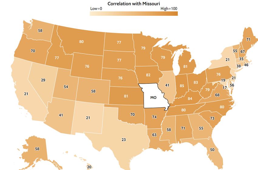
Judgment and Decision Making, Vol. 15, No. 5, September 2020 Information, incentives, and goals in election forecasts 867

so these 10 national elections would not represent 500 in- culated using the normal cumulative distribution function:
dependent data points. This is not to say that calibration Φ((0.54 − 0.517)/0.02) = 0.875.
is a bad idea, just that it must be undertaken carefully, and Now suppose that our popular vote forecast is off by
95% intervals will necessarily depend on assumptions about half of a percentage point. Given all our uncertainties,
the tail behavior of forecasts that cannot be directly checked it would seem too strong to claim we could forecast to
from past data. For a simple example, suppose we had data that precision anyway. If we bump Biden’s predicted two-
on 10 independent events, each forecast with probability 0.7. party vote down to 53.5%, his win probability drops to
Then we would expect
 p to see a 0.7 success rate, but with a Φ((0.535 − 0.517)/0.02) = 0.816.
standard error of 0.7 · 0.3/10 = 0.14, so any success rate Thus, a shift of 0.5% in Biden’s expected vote share corre-
between, say, 0.5 and 0.9 would be consistent with calibra- sponds to a change of 6 percentage points in his probability of
tion. It would be possible here to diagnose only extreme winning. Conversely, a change in 1% of win probability cor-
cases of miscalibration. responds to a 0.1% percentage point share of the two-party
 Boice and Wezerek (2019) present a graph assessing cal- vote. There is no conceivable way to pin down public opin-
ibration of forecasts from Fivethirtyeight based on hundreds ion to a one-tenth of a percentage point, which suggests that,
of thousands of election predictions, but these represent pre- not only is it meaningless to report win probabilities to the
dictions of presidential and congressional elections for every nearest tenth of a percentage point, it’s not even informative
state on every date that forecasts were available; ultimately to present that last digit of the percentage.
these are based on a much smaller number of events used On the other hand, if we round to the nearest 10 percentage
to measure the calibration, and these events are themselves points so that 87% is reported as 90%, this creates other
occurring in only a few election years. As a result, trying to difficulties at the high end of the range — we would not want
identify over- or underconfidence of forecasts is inherently to round 96% to 100% — and also there will be sudden jumps
speculative, as we do not typically have enough information when the probability moves from 90% to 80%, say. For
to make detailed judgments about whether a political fore- the 2020 election, both the Economist and Fivethirtyeight
casting method is uncalibrated — or, to be precise, to get compromised and rounded to the nearest percentage point
a sense of under what conditions a forecast will be over or but then summarized these numbers in ways intended to
underconfident. This is not to say that reflecting on goals and convey uncertainty and not lead to overreaction to small,
incentives in election forecasting is futile; on the contrary, meaningless changes in both win probabilities and estimates
we think doing so can be informative for both forecast con- of vote share.
sumers and researchers, and we discuss possible incentives One can also explore how the win probability depends
in Section 3. on the uncertainty in the vote. Again continuing the above
 example, suppose we increase the standard deviation of the
 national vote from 2 to 3 percentage points. This decreases
2.2 Win probabilities the win probability from 0.875 to Φ((0.54 − 0.517)/0.03) =
There are also tensions related to people’s desire for precise 0.77.
win probabilities and what these probabilities mean. There
is a persistent confusion between forecast vote share and win 2.3 Using anomalous predictions to improve a
probabilities. A vote share of 60% is a landslide win, but
 model
a win probability of 60% corresponds to an essentially tied
election. For example, as of September 1, the Economist Forecasters can use the uncertainty in their predictions as
model was forecasting a 54% share of the two-party vote for benchmarks for iterating on their models. For example, at the
Biden and an 87% chance of him winning in the electoral time of writing this article in September 2020, the Fivethir-
college. tyeight site gives a 95% predictive interval of (42%, 60%) for
 How many decimal places does it make sense to report Biden’s share of the two-party vote in Florida, and also pre-
the win probability? We work this out using the following dicts that Trump, in the unlikely event that he wins California,
simplifying assumptions: (1) each candidate’s share of the has a 30% chance of losing in the electoral college. Neither
national two-party vote is forecast with a normal distribution, of these predictions seem plausible, at least to us. That is,
and (2) as a result of imbalances in the electoral college, the Florida interval seems too wide given that at the time of
Biden wins the election if and only if he wins at least 51.7% writing this article, Biden is at 52% in the polls there and
of the two-party vote. Both of these are approximations, at 54% in the national polls and in our fundamentals-based
but generalizing to non-normal distributions and aggregating forecast, and Florida is a swing state. Other fundamentals-
statewide forecasts will not really affect our main point here. based forecasts put the election at closer to 50–50, but even
 Given the above assumptions, suppose the forecast of there we do not see how one could plausibly get to a Trump
Biden’s national vote share is 54% with a standard deviation landslide in that state. In contrast, the California conditional
of 2%. Then the probability that Biden wins can be cal- prediction made by Fivethirtyeight seems too pessimistic on

Judgment and Decision Making, Vol. 15, No. 5, September 2020 Information, incentives, and goals in election forecasts 868

Trump’s chances: if the president really were to win that 2.4 Visualizing uncertainty
state, this would almost certainly happen in a Republican
 There is a literature on communicating probability state-
landslide (only Hawaii and Washington D.C. lean more to-
 ments (for example, Gigerenzer & Hoffrage, 1995, Spiegel-
ward the Democrats), in which case it’s hard to imagine him
 halter, Pearson & Short, 2011) but it remains a challenge
losing in the country as a whole.
 to express election forecasts so they will be informative to
 Both the extremely wide Florida interval and the inappro-
 political junkies without being misinterpreted by laypeople.
priately equivocal prediction conditional on a Trump victory
 In communicating the rationale behind Fivethirtyeight’s dis-
in California that we observe seem to reveal that the Fivethir-
 plays, Wiederkehr (2020) writes:
tyeight forecast has a too-low correlation among state-level
uncertainties. Their joint prediction doesn’t appear to ac- Our impression was that people who read a lot
count for the fact that either event — Biden receiving only of our coverage in the lead-up to 2016 and spent
42% in Florida or Trump winning California — would in all a good amount of time with our forecast thought
probability represent a huge national swing. we gave a pretty accurate picture of the election
 Suppose you start with a forecast whose covariances across . . . People who were looking only at our top-line
states are too low, in the sense of not fully reflecting the un- forecast numbers, on the other hand, thought we
derlying correlations of opinion changes across states, and bungled it. Given the brouhaha after the 2016
you want this model to have a reasonable uncertainty at the election, we knew we had to thoughtfully approach
national level. To achieve this, you need to make the uncer- how to deliver the forecast. When readers came
tainties within each state too wide, to account for the variance looking to see who was favored to win the election,
reduction that arises from averaging over the 50 states. Thus, we needed to make sure that information lived in a
implausible state-level predictions may be artifacts of too- well-designed structure that helped people under-
low correlations along with the forecasters’ desire to get an stand where those numbers are coming from and
appropriately wide national forecast. Low correlations can what circumstances were affecting them.
also arise if you start with a model with high correlations
 Given that probability itself can be difficult for laypeople
and then add independent state errors with a long-tailed dis-
 to grasp, it will be especially challenging to communicate
tribution.
 uncertainty in a complex multivariate forecast. One message
 One reason we are so attuned to this is that a few weeks
 from the psychology literature is that natural frequencies
after we released our first model of the election cycle for the
 provide a more concrete impression of probability. Natural
Economist, we were disturbed at the narrowness of some of
 frequencies work well for examples such as disease risk (“Out
its national predictions. In particular, at one point the model
 of 10,000 people tested, 600 will test positive, out of whom
had Biden with a 99% chance of winning the popular vote.
 150 will actually have the disease”).
Biden was clearly in the lead; at the same time, we thought
 A frequency framing becomes more abstract when applied
that 99% was too high a probability. Seeing this implausible to a single election. Formulations such as “if this election
predictive interval motivated us to refactor our model, and we were held 100 times” or “in 10,000 simulations of this elec-
found some bugs in our code and some other places where tion” are not so natural. Still, frequency framing may better
the model could be improved — including an increase in emphasize lower probability events that readers are tempted
between-state correlations, which increased uncertainty of to ignore with probability statements. When faced with a
national aggregates. The changes in our model did not have probability, it can be easier to round up (or down) than to
huge effects — not surprisingly given that we had tested our form a clear conception of what a 70% chance means. We
earlier model on 2008, 2012, and 2016 — but the revision did won’t have more than one Biden versus Trump election to
lower Biden’s estimated probability of winning the popular test a model’s predictions on, but we can imagine applying
vote to 98%. This was still a high value, but it was consistent predictions to a series of elections.
with the polling and what we’d seen of variation in the polls A growing body of work in computer science has pro-
during the campaign. posed and studied static and dynamic visual encodings for
 The point of this discussion is not to say that the Fivethir- uncertainty. While much of this work has focused on visual-
tyeight forecast is “wrong” and that the Economist model izing uncertainty in complex high dimensional data analyzed
is “right” — they are two different procedures, each with by scientists, some new uncertainty visualization approaches
their own strengths and weaknesses — but rather that, in ei- have been proposed to support understanding among broader
ther case, we can interrogate a model’s predictions to better audiences, several of which use a visual frequency fram-
understand its assumptions and relate it to other available ing. For example, animated hypothetical outcome plots
information or beliefs. Other forecasters can and possibly (Hullman, Resnick & Adar, 2015) present random draws
do undertake such interrogations to fine-tune their models from a distribution over time, while quantile dotplots dis-
over time, both during election cycles and in between. cretize a density into a set of 20, 50, or 100 dots (Kay et

Judgment and Decision Making, Vol. 15, No. 5, September 2020 Information, incentives, and goals in election forecasts 869

Figure 1: Some displays of uncertainty in presidential election forecasts. Top row: 2016 election needle from the New York
Times and map icon array from Fivethirtyeight in 2020. Center row: time series of probabilities from Fivethirtyeight in 2012
and their dot distribution in 2020. Bottom row: time series of popular vote projections and interactive display for examining
between-state correlations from the Economist in 2020. No single visualization captures all aspects of uncertainty, but a set
of thoughtful graphics can help readers grasp uncertainty and learn about model assumptions over time.

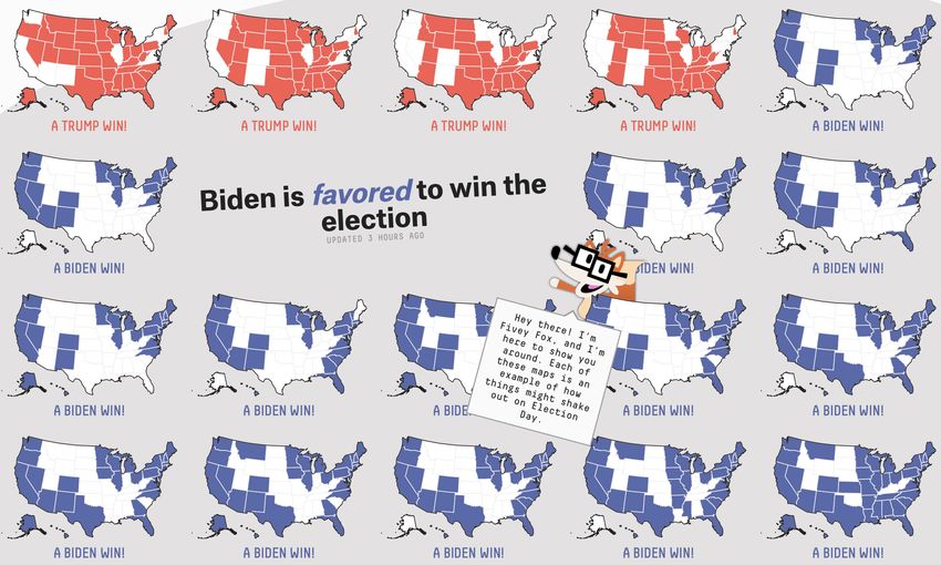
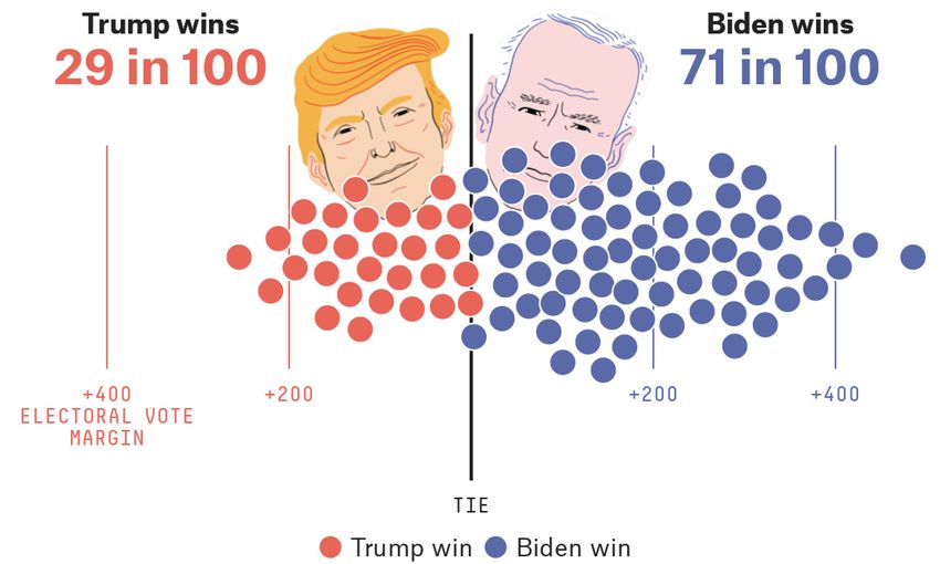
Judgment and Decision Making, Vol. 15, No. 5, September 2020 Information, incentives, and goals in election forecasts 870

al., 2016). Controlled experiments aimed at understand- dle was an effective example of animation, using a shaded
ing how frequency-framed visualizations affect judgments gauge in the background to show plausible outcomes ac-
and decisions made by laypeople provide a relevant base cording to the model, with the needle itself jumping to a new
of knowledge for forecasters. For example, multiple stud- location within the central 50% interval every fraction of a
ies compare frequency visualizations to more conventional second. The needle conveyed uncertainty in a way that was
displays of uncertainty. Several of these studies find these visceral and hard to ignore, but readers and journalists alike
tools enable laypeople to make more accurate probability expressed disapproval and even anger at its use (McCormick,
estimates and even better decisions as defined against a ra- 2016). While it was not clear to many readers what exactly
tional utility-optimal standard (Fernandes et al., 2018, Kale, drove each movement of the needle, we think expectations
Kay & Hullman, 2020) as compared to those who are given were likely a bigger contributor to the disapproval: the nee-
error bars and variations on static, continuous density plots. dle was very different from the standard presentations of
 Other studies suggest that the type of uncertainty informa- forecasts that had been used up until election night. Readers
tion reported (for example, a predictive interval rather than who had relied on simple heuristics to discount uncertainty
a confidence interval) is more consequential in determining shown in static plots were suddenly required to contend with
perceptions and decisions (Hofman, Goldstein & Hullman, uncertainty, at a time when they were already anxious.
2020). One reason that it is challenging to try to generalize A more subtle frequency visualization is the grid of maps
these findings from laboratory experiments is that people are used as the header for Fivethirtyeight’s forecasting page,
likely to adapt various types of heuristics when confronted with the number of blue and red maps representing possi-
with uncertainty visualizations, and these heuristics can vary ble combinations of states leading to a Biden or Trump win
based on context. For example, when faced with a visual- according to the probability assigned by the forecast. Vi-
ization showing a difference between two estimates with sualization researchers have called grids of possible worlds
uncertainty, many people tend to look at the visual distance “pangloss plots” (Correll & Gleicher, 2014), representing a
between mean estimates and use it to judge the reliability slightly more complex example of icon arrays, which have
of the difference (Hullman, Resnick & Adar, 2015, Kale, long been used to communicate probabilities to laypeople
Kay & Hullman, 2020). When someone is already under a in medical risk communication (Ancker et al., 2006). The
high cognitive load, these heuristics, which generally act to Economist display designers also experimented with an icon-
suppress uncertainty, may be even more prevalent (Zhou et style visualization for communicating risk or “risk theater”,
al., 2017). which shaded a percentage of squares in a grid blue or red to
 There’s even some evidence that people apply heuristics reflect the percentage change that either candidate wins the
like judging visual distances to estimate effect size even electoral college.
when given what statisticians and designers might view as For illustrating the time series of predictions during the
an optimal uncertainty visualization for their task. A recent campaign, the Fivethirtyeight lineplot is clear and simple,
study found that less than 20% of people who were given but, as noted in Section 2.2, it presented probabilities to an
animated hypothetical outcome plots, which directly express inappropriately high precision given the uncertainties in the
probability of superiority (the probability that one group inputs to the model. In addition, readers who focus on a plot
will have a higher value than another), figured out how to of win probability may fail to understand how this maps to
properly interpret them (Kale, Kay & Hullman, 2020). So vote share (Urminsky & Shen, 2019, Westwood, Messing &
even when a visualization makes uncertainty more concrete, Lelkes, 2020).
it will also matter how forecasters explain it to readers, how Fivethirtyeight’s dot distribution shows another frequency
much attention readers have to spend on it, and what they visualization. In contrast to the map icon array, the dot dis-
are seeking from the information. play also conveys information about how close the model
 Some recent research has tried to evaluate how the infor- predicts the electoral college outcome to be. Readers may
mation highlighted in a forecast display — win probability be confused about how this particular set of 100 dots was
or vote share — may affect voting decisions in a presidential chosen, and the display loses precision compared to a contin-
elections (Westwood, Messing & Lelkes, 2020, Urminsky & uous display, but it has the advantage of making probability
Shen, 2019). One reason why studying the impact of visu- more concrete through frequency. Indeed, it was through
alization choices on voting decisions is challenging is that these visualizations that we noticed the problematic state-
voting is an act of civic engagement more than an individual level forecasts discussed in Section 2.3.
choice. Decision making in an economic or medical setting The Economist time series plot of estimated vote prefer-
is more subject to probabilistic analysis because the potential ence has the appealing feature of being able to include the
losses and benefits there are more clear. poll data and the model predictions on the same scale. Here
 Figure 1 shows uncertainty visualizations from recent readers may be likely to judge how close the race is based
election campaigns that range from frequency based to more on how far apart the two candidates’ forecasts are from one
standard interval representations. The New York Times nee- another within the total vertical space of the -axis (Kale,

Judgment and Decision Making, Vol. 15, No. 5, September 2020 Information, incentives, and goals in election forecasts 871

Kay & Hullman, 2020), rather than trying to understand how on reading charts and pointing to further information on the
close the two percentages are in other ways, such as by com- forecast, Fivey also seems intended to remind readers of the
paring to prior elections. Shaded 95% confidence intervals, potential for very low probability events that run counter
which barely overlap in this particular case, help convey how to the forecast’s overall trend, for example reminding read-
sure the model is that Biden will win. If the intervals were to ers that “some of the bars represent really weird outcomes,
overlap more, people’s heuristics for interpreting how “sig- but you never know!” as they examine a plot showing many
nificant” the difference between the candidates is might be possible outcomes produced by the forecast.
more error prone (Belia et al., 2005). The display does not The problem is that how strongly these statements should
map directly onto win probability or even electoral college be worded and how effective they are is difficult to assess,
outcomes and so may be consulted less by readers wanting because there is no normative interpretation to be had. More
answers, but, as discussed in Section 2.2, we believe that vote useful narrative accompaniments to forecasts would include
proportions are ultimately the best way to understand fore- some mention of why there are unknowns that result in un-
cast uncertainty, given that short-term swings in opinions certainty. This is not to say that tips such as those of Fivey
and votes tend to be approximately uniform at the national Fox are a bad idea, just that, as with other aspects of com-
level. Electoral college predictions are made available in a munication, their effectiveness is hard to judge and so we are
separate plot. relying on intuition as much as anything else in setting them
 Finally, the Economist’s display includes an interactive up and deploying them.
choropleth map that allows the reader to select a state and Communicating uncertainty is not just about recognizing
view how correlated the model expects its voting outcomes its existence; it is also about placing that uncertainty within
to be with other states via shading. This map alerts readers a larger web of conditional probability statements. In the
to an aspect of election forecasting models that often goes election context, these could relate to shifts in the polls or
unnoticed — the importance of between-state correlations to unexpected changes in underlying economic and political
in prediction — and lets them test their intuitions against the conditions, as well as the implicit assumption that factors not
model’s assumptions. included in the model are irrelevant to prediction. No model
 As in presenting model predictions in general, it is good can include all such factors, thus all forecasts are conditional.
to present multiple visualizations to capture different aspects We try our best to capture forecast uncertainty by calibrating
of data and the predictive distribution as they change over the residual error terms on past elections, but every election
time. Plots showing different components of a forecast can introduces something new.
implicitly convey information about the model and its as-
sumptions, and both Fivethirtyeight and the Economist do
well by displaying many different looks at the forecast, along 2.6 Prediction markets
with supplying probabilistic simulations available for down-
load. A completely different way to evaluate forecasts and think
 about their uncertainties is to compare them to election bet-
 ting markets. In practice, we would not expect such markets
2.5 Other ways to communicate uncertainty to have the martingale property; as Aldous (2013) puts it,
It is difficult to present an election forecast without some “compared to stock markets, prediction markets are often
narrative and text expression of the results. But effectively thinly traded, suggesting that they will be less efficient and
communicating uncertainty in text might be even harder than less martingale-like.” Political betting markets, in partic-
visualizing probability. Research has found that the proba- ular, will respond to a series of new polls and news items
bility ranges people assign to different text descriptions of throughout the campaign. The markets can overreact to polls
probability such as “probable”, “nearly certain”, and so forth, or can fail in the other direction by self-reinforcing, thus para-
vary considerably across people (Wallsten, Budescu & Rap- doxically not making the best use of new data (Erikson &
paport, 1986, Budescu, Weinberg & Wallsten, 1988). Wlezien, 2008, Gelman & Rothschild, 2016a). That said,
 For uncertainty that can’t be quantified because it involves markets offer a different sort of data than polls and funda-
unknowns such as the credibility of assumptions, it may help mentals, and we should at least be aware of how these signals
to resort to qualitative text expressions like “there is some un- can disagree.
certainty around these results due to X.” Some research sug- During the 2020 campaign, prediction markets in the 2020
gests that readers take these qualitative statements more seri- campaign have consistently given Biden an implicit win
ously than they do quantitative cues (van der Bles, Freeman probability in the 50–60% range, compared to poll-based
& Spiegelhalter, 2019). Fivethirtyeight’s 2020 forecast in- forecasting models that have placed the Democrat’s chance
troduces “Fivey Fox”, a bespectacled, headphones-wearing, of winning to be in the 70–90% range. That said, this direct
sign-holding cartoon in the page’s margins who delivers ad- interpretation of the probabilities for winner-take-all prices
vice directly to readers. In addition to providing guidance is not entirely straightforward (Manski 2006).

Judgment and Decision Making, Vol. 15, No. 5, September 2020 Information, incentives, and goals in election forecasts 872

 This discrepancy between statistical forecasts and markets isons between forecasters may shift perceived responsibility,
can be interpreted in various ways. The market odds can and the public may bring expectations that news outlets con-
represent a mistake of bettors who are overreacting to the tinually provide new information. We discuss how these
surprise outcome from 2016. Another possibility is that factors combine to make forecasters’ incentives complex.
poll aggregation fails to account for systematic biases or the
possibility of large last-minute opinion changes, in which 3.1 Incentives for overconfidence
case the markets could motivate changes in the forecasting
models. Less than a month before the 2016 election, cartoonist Scott
 It is unclear exactly how we would incorporate betting Adams wrote, “I put Trump’s odds of winning in a landslide
market information into a probabilistic forecast. As noted, back to 98%”, a prediction that was evidently falsified — it
the markets are thin and, when state-level markets are also would be hard to call Trump’s victory, based on a minority of
included, the resulting multivariate probabilities can be in- the votes, as a “landslide” — while, from a different corner
coherent. We can think of the betting odds as a source of of the political grid, neuroscientist Sam Wang gave Hillary
external information, alongside other measures such as re- Clinton a 98% chance of winning in the electoral college,
ports of voter enthusiasm, endorsements, money raised, and another highly confident prediction that did not come to pass
features such as the coronavirus epidemic that could affect (Adams, 2016; Wang, 2016). These failures did not remove
voter turnout in ways that are unique to the current elec- either of these pundits from the public eye. As we wrote in
tion year and so are difficult to directly incorporate into a our post-election retrospective (Gelman & Azari, 2017):
forecasting model.
 There’s a theory that academics such as ourselves
 Another reason that polls can differ from betting odds
 are petrified of making a mistake, hence we are
is that surveys measure vote intention, whereas the market
 overcautious in our predictions; by contrast, the
applies to official vote totals; as discussed in Section 1.4,
 media (traditional news media and modern social
vote suppression and discrepancies in vote counts are not
 media) reward boldness and are forgiving of fail-
addressed by existing prediction models that use polls and
 ure. This theory is supported by the experiences
fundamentals. In theory, and perhaps in practice, markets
 of Sam Wang (who showed up in the New York
can include information or speculation about such factors
 Times explaining the polls after the election he’d
that are not included in the forecasts.
 so completely biffed) and Scott Adams (who tri-
 umphantly reported that his Twitter following had
 reached 100,000).
3 The role of incentives
 There are other motivations for overconfidence. The typ-
Election forecasting might be an exception to the usual rule of ical consumer of an election forecast just wants to know
de-emphasizing uncertainty in data-driven reporting aimed who is going to win; thus there is a motivation for the pro-
at the public, such as media and government reporting. Fore- ducer of a forecast to fulfill that demand which is implicit
casters appear to be devoting more effort to better express- in the conversation, in the sense of Grice (1975). And, even
ing uncertainty over time, as illustrated by the quote leading without any such direct motivation for overconfidence, it is
off Section 2.4 from Wiederkehr (2020), discussing choices difficult for people to fully express their uncertainty when
made in displaying predictions for 2020 in response to crit- making probabilisitic predictions (Alpert & Raiffa, 1982,
icisms of the ways in which forecasts had been presented in Erev, Wallsten & Budescu, 1994). If calibrated intervals are
the previous election. too hard to construct, it can be easier to express uncertainty
 The acknowledgment that it can be risky to present num- qualitatively than to get a good quantitative estimate of it.
bers or graphs that imply too much precision may be a sign Another way to look at overconfidence is to consider the
that forecasters are incentivized to express wide intervals, extreme case of just reporting point forecasts without any un-
perceiving the loss from the interval not including the ulti- certainty at all. Rationales for reporting point estimates with-
mate outcome to be greater than the gain from providing a out uncertainty include fearing that uncertainty information
narrow, precise interval. We have also heard of news editors will imply unwarranted precision in estimates (Fischhoff,
not wanting to “call the race” before the election happens, 2012); feeling that there are no good methods to commu-
regardless of what their predictive model says. Compared nicate uncertainty (Hullman, 2019); thinking that the pres-
to other data reporting, a forecast may be more obvious to ence of uncertainty is common knowledge (Fischhoff, 2012);
readers as a statement issued by the news organization, so thinking that non-expert audiences will not understand the
the uncertainty also has to be obvious, despite readers’ ten- uncertainty information and resort to “as-if optimization”
dencies to try to ignore it. At the same time, reasons to that treats probabilistic estimates as deterministic regard-
underreport uncertainty are pervasive in data reporting for less (Fischhoff, 2012, Manski, 2019); thinking that not pre-
broad audiences (Manski, 2019), the potential for compar- senting uncertainty will simplify decision making and avoid

Judgment and Decision Making, Vol. 15, No. 5, September 2020 Information, incentives, and goals in election forecasts 873

overwhelming readers (Hullman, 2019, Manski, 2019); and cause there are many players, so any given forecaster is less
thinking that not presenting uncertainty will make it easier exposed; also, once consumers embraced poll aggregation,
for people to coordinate beliefs (Manski, 2019). forecasting became a logical next step.
 There are also strategic motivations for forecasters to min- Regarding predictions for 2020, the creator of the Fivethir-
imize uncertainty. Expressing high uncertainty violates a tyeight forecast writes, “We think it’s appropriate to make
communication norm and can cause readers to distrust the fairly conservative choices especially when it comes to the
forecaster (Hullman, 2019, Manski, 2018). This is some- tails of your distributions. Historically this has led 538
times called the auto mechanic’s incentive: if you are a to well-calibrated forecasts (our 20%s really mean 20%)”
mechanic and someone brings you a car, it is best for you (Silver, 2020b). But making predictions conservative corre-
to confidently diagnose the problem and suggest a remedy, sponds to increasing the widths of intervals, playing it safe
even if you are unsure. Even if your diagnosis turns out to be by including extra uncertainty. Characterizing a forecast-
wrong, you will make some money; conversely, if you hon- ing procedure as conservative implies an attitude of risk-
estly tell the customer you don’t know what is wrong with aversion, being careful to avoid the outcome of the pre-
the car, you will likely lose this person’s business to another, dictive interval not including the actual election result. In
less scrupulous, mechanic. other words, conservative forecasts should lead to undercon-
 Election forecasters are in a different position than auto fidence: intervals whose coverage is greater than advertised.
mechanics, in part because of the vivid memory of polling And, indeed, according to the calibration plot shown by
errors such as 1948 and 2016 and in part because there Boice and Wezerek (2019) of Fivethirtyeight’s political fore-
is a tradition of surveys reporting margins of error. Still, casts, in this domain their 20% really means 14%, and their
there is room in the ecosystem for bold forecasters such as 80% really means 88%. As discussed in Section 2.1, these
Lichtman (1996), who gets a respectful hearing in the news numbers are based on a small number of elections so we
media every four years (for example Stevenson, 2016; Raza shouldn’t make too much of them, but this track record is
& Knight, 2020) with his “surefire guide to predicting the consistent with Silver’s goal of conservatism, leading to un-
next president”. derconfidence. Underconfident probability assessments are
 a rational way to hedge against the reputational loss of having
 the outcome fall outside a forecast interval, and arguably this
3.2 Incentives for underconfidence
 cost is a concern in political predictions more than in sports,
One incentive to make prediction intervals wider, and to keep as sports bettors are generally comfortable with probabilities
predictive probabilities away from 0 and 1, is an asymmetric and odds. And Fivethirtyeight’s probabilistic forecasts for
loss function. A prediction that is bold and wrong can dam- sporting events do appear to be calibrated (Boice & Wezerek,
age our reputation more than we would gain from one that 2019).
is bold and correct. To put it another way: suppose we were Speaking generally, some rationales for unduly wide in-
to report only 50% intervals. Outcomes that fall within the tervals — underconfident or conservative forecasts — are
interval will look from the outside like “wins” or successful that they can motivate receivers of the forecast to diver-
predictions; observations that fall outside look like failures. sify their behavior more, and they can allow forecasters to
From that perspective there is a clear motivation to make avoid the embarrassment that arises when they predict a
50% intervals that are, say, 70% likely to cover the truth, high-probability win for a candidate and the candidate loses.
as this will be expected to supply a steady stream of wins This interpretation assumes that people have difficulty un-
(without the intervals being so wide as to appear useless). derstanding probability and will treat high probabilities as if
 In 1992, one of us constructed a hierarchical Bayesian they are certainties. Research has shown that readers can be
model to forecast presidential elections, not using polls but less likely to blame the forecaster for unexpected events if
only using state and national level economic predictors as uncertainty in the forecast has been made obvious (Joslyn &
well as some candidate-level information, with national, re- LeClerc, 2012).
gional, and state-level error terms. Our goal was not to
provide real-time forecasts but just to demonstrate the pre-
 3.3 Incentives in competing forecasts
dictability of elections; nonetheless, just for fun we used our
probabilistic forecast to provide a predictive distribution for Incentives could get complicated if forecasters expect “du-
the electoral college along with various calculations such as eling certitudes” (Manski, 2011), cases where multiple fore-
the probability of an electoral college tie and the probabil- casters are predicting a common outcome. For example,
ity that a vote in any given state would be decisive. One suppose a forecaster knows that other forecasters will likely
reason we did not repeat this exercise in subsequent elec- be presenting estimates that will differ from each other, at
tions is that we decided it could be dangerous to be in the least to some extent. This could shift some of the perceived
forecasting business: one bad-luck election could make us responsibility for getting the level of uncertainty calibrated
look like fools. It is easier to work in this space now be- to the group of forecasters. Maybe in such cases each fore-