Informing sea otter reintroduction through habitat and human interaction assessment
←
→
Page content transcription
If your browser does not render page correctly, please read the page content below
Vol. 44: 159–176, 2021              ENDANGERED SPECIES RESEARCH
                                                                                               Published February 25
 https://doi.org/10.3354/esr01101             Endang Species Res

                                                                                                 OPEN
                                                                                                 ACCESS

          Informing sea otter reintroduction through
           habitat and human interaction assessment
                    Dominique V. Kone1, 4,*, M. Tim Tinker2, Leigh G. Torres3
          1
         College of Earth, Ocean, and Atmospheric Science, Marine Mammal Institute, Oregon State University,
                                2030 SE Marine Science Drive, Newport, OR 97365, USA
   2
    Department of Ecology and Evolutionary Biology, University of California, Santa Cruz, Santa Cruz, CA 95064, USA
 3
  Department of Fisheries and Wildlife, Marine Mammal Institute, Oregon State University, 2030 SE Marine Science Drive,
                                                Newport, OR 97365, USA
              4
               Present address: California Ocean Science Trust, 1111 Broadway, Oakland, CA 94607, USA

       ABSTRACT: Sea otters Enhydra lutris have been absent from Oregon, USA, following their extir-
       pation over a century ago. Stakeholder groups and native tribes are advocating for reintroduction
       to restore historic populations. We investigated the potential for successful reintroduction by: (1)
       estimating expected equilibrium sea otter densities as a function of habitat variables to assess sea
       otter habitat in Oregon; and (2) spatially relating areas of high expected densities to human activ-
       ities (e.g. fisheries, recreation, vessel activity, protected areas) to anticipate potential disturbance
       or fishery resource competition. We estimated that 4538 (1742−8976; 95% CI) sea otters could
       exist in Oregon, with higher expected abundance (N = 1551) and densities (x– = 2.45 km−2) within
       the southern region. Most core habitat areas (97%), representing clusters of high expected densi-
       ties, overlapped with some form of human activity. While commercial shipping and tow lanes
       overlapped little (1%) with core habitat areas, recreational activities (58%) and fisheries (76%)
       had a higher degree of overlap, posing higher disturbance risk. We anticipate higher resource
       competition potential with the commercial red sea urchin fishery (67% of harvest areas) than the
       commercial Dungeness crab fishery (9% of high-catch crabbing grounds). Our study presents the
       first published carrying capacity estimate for sea otters in Oregon and can provide population
       recovery targets, focus attention on ecological and socioeconomic considerations, and help to
       inform a recovery plan for a resident sea otter population. Our findings suggest current available
       habitat may be sufficient to support a sea otter population, but resource managers may need to
       further investigate and consider whether current human activities might conflict with reestablish-
       ment in Oregon, if plans for a reintroduction continue.

       KEY WORDS: Sea otter · Enhydra lutris · Oregon · Reintroduction · Habitat · Carrying capacity ·
       Fisheries · Conservation

                  1. INTRODUCTION                             (Clapham et al. 1999) and over-fished cod stocks
                                                              along the US northeast coast (Hutchings & Myers
   Throughout history, humans have exploited wild-            1994, Myers et al. 1997). As biodiversity loss has
life populations, and these activities may partially          accelerated, the importance of species diversity to
explain Earth’s sixth mass extinction (Barnosky et al.        ecosystem function, resilience, and services has
2011, Dirzo et al. 2014). Well-known examples of              become apparent (Cardinale et al. 2002, Elmqvist et
exploitive practices include near collapses in global         al. 2003, Downing & Leibold 2010). Biodiversity loss
whale populations due to international whaling                thus represents a prominent threat to environmental
                                                              © The authors 2021. Open Access under Creative Commons by
*Corresponding author: dom.kone@oceansciencetrust.org         Attribution Licence. Use, distribution and reproduction are un-
                                                              restricted. Authors and original publication must be credited.
                                                              Publisher: Inter-Research · www.int-res.com
160 Endang Species Res 44: 159–176, 2021 sustainability. Recovery of at-risk species, particu- species will reestablish in their release area (Sarrazin larly species vital to ecosystem function, can help & Barbault 1996). Habitat suitability assessments can maintain ecosystem integrity (Soulé et al. 2003). reduce this uncertainty by identifying areas of unoc- Environmental managers enlist a range of strategies cupied habitats that are likely to sustain the intro- to facilitate at-risk species recovery, such as estab- duced species and foster population growth over lishing protected areas, moving threatened popula- time (Cheyne 2006). Predator populations and popu- tions into captivity, or conducting reintroductions lation growth are often limited by prey availability. and reinforcements (Briggs 2009). Therefore, habitat models can be used to identify and Sea otters Enhydra lutris were once distributed predict areas of unoccupied habitats that are likely to along most North Pacific Ocean coastlines from Japan contain adequate prey to sustain the predator. to Baja California, Mexico, but were extirpated from Sea otters have been absent from Oregon waters most of their historic range during the peak of the for more than 100 yr, during which time nearshore maritime fur trade from the mid-1700s to mid-1800s habitats have experienced substantial change. A vari- (Kenyon 1969). Recovery occurred slowly over the ety of human activities now occur along the Oregon first half of the 20th century; however, a significant coast, including fisheries, recreation, and shipping boost to recovery occurred in the late 1960s when (Norman et al. 2007, LaFranchi & Daugherty 2011), resource managers translocated sea otters from which could disturb sea otters or make habitats less Amchitka Island and Prince William Sound, Alaska, hospitable. At present there has been no systematic to Southeast Alaska, British Columbia, Washington, assessment of the potential for sea otters to reestab- and Oregon. Most of these translocation efforts were lish in Oregon. Using predictive models to evaluate successful, and populations in these areas are now the potential for sea otter recovery in different sites abundant and thriving. A notable exception was the can help fill this knowledge gap; such models require translocation effort to Oregon, where the founding an understanding of habitat features that facilitate population gradually declined from reintroduction in effective sea otter foraging and knowledge of current 1970−1971 (N = 93 otters) to 1981, when only 1 otter nearshore habitats in Oregon. Luckily, sea otter habi- was observed during routine surveys, after which the tat-use patterns and foraging activities are well doc- population was expected to disappear (Jameson et umented in other regions (e.g. Ostfeld 1982, Laidre et al. 1982). No consensus exists for the cause of failure al. 2009, Hughes et al. 2013, Lafferty & Tinker 2014), of the Oregon population, but several hypothesized and this information can be leveraged for considera- factors include lack of appropriate habitat or prey, tion of the potential for sea otter recovery in Oregon. human disturbance, or sea otter emigration due to Sea otters are typically found within shallow and homing behavior (Jameson et al. 1982). Presently, intertidal rocky habitats, where they forage for ben- stakeholder groups and native tribes are advocating thic macroinvertebrates such as sea urchins, sea for a second attempt at sea otter reintroduction to snails, bivalves, and crabs (Estes et al. 1982, Ostfeld Oregon, arguing that this action could achieve sev- 1982, Laidre & Jameson 2006, Newsome et al. 2009). eral objectives, including: (1) aiding recovery efforts Canopy-forming and understory macroalgae (i.e. for a species of conservation concern; (2) restoring kelp, seaweed) also provide important habitat for coastal food web structure and function; (3) provision- prey species as well as protected resting habitat for ing ecosystem services, including economic or intrin- sea otters (Estes & Palmisano 1974, Estes et al. 1982, sic/recreational benefits; and (4) restoring lost cul- Nicholson et al. 2018). In addition to rocky and kelp- tural and tribal traditions and ecological connections. dominated habitats, sea otters also use soft-sediment Species reintroductions represent an important habitats on the outer coast and within estuaries tool for managers charged with recovering at-risk (Riedman & Estes 1990, Hughes et al. 2013, 2019, species (Clark & Westrum 1989, Seddon et al. 2007). Hale et al. 2019). Sea otters have been infrequently There have been several notable cases where observed hauling out on shore to rest, groom, and translocations have contributed to species recovery, forage. This behavior appears to be more common including the previously mentioned sea otter translo- on marshes within Elkhorn Slough, California, and cations across the North Pacific Ocean, red deer on sand and mud bars in Alaska, and is much less Cervus elaphus to central Portugal (Valente et al. observed along outer coastal shorelines (Kenyon 2017), and gray wolves Canis lupus to Yellowstone 1969, Garshelis & Garshelis 1984, Faurot 1985, Green National Park, USA (Smith & Guernsey 2002, Ripple & Brueggeman 1991, Eby et al. 2017). The seaward & Beschta 2003). Species reintroductions are also distribution of sea otters is limited by their maximum risky because uncertainty surrounds whether the diving capacity of 100 m depth (Bodkin et al. 2004,
Kone et al.: Sea otter reintroduction in Oregon                              161

Thometz et al. 2016), although most dives occur                costly. It is unclear whether, and to what degree, dis-
within 40 m depth. Within their nearshore distribu-            turbance-induced behavior and physiological re-
tion, sea otter densities have a non-linear relation-          sponses in sea otters are great enough to produce
ship with depth, where densities peak around a                 population-level consequences. Regardless, human
model depth of 15 m, and gradually decline as depth            disturbance has been, and continues to be, a concern
increases or decreases (Tinker et al. 2017). The slope         for sea otter survival and conservation (US Fish and
and width of the continental shelf can dictate how             Wildlife Service 2003) and should be accounted for
dense or spread out populations are across space               when deciding if and where sea otters should be
(Tinker et al. 2021). Relative to other marine preda-          reintroduced in Oregon.
tors, sea otters have extremely high metabolisms and              Fisheries add a further complication due to con-
almost no capacity for energy storage in fat tissue,           cerns regarding competition and ecosystem impacts
and thus require anywhere from 25 to 30% of their              of sea otter foraging on certain shellfish species im-
own body weight in food every day (Costa & Kooy-               portant to fisheries (Johnson 1982). Sea otters exhibit
man 1982, Riedman & Estes 1990). Their extreme                 strong top-down pressures by reducing prey densi-
dependency on high energy prey means identifying               ties and size via predation (Estes et al. 1978, Estes &
high quality foraging habitat within their depth limits        Duggins 1995), and sea otter-driven reductions in
is imperative to facilitating successful reintroduction.       fishery-dependent prey species have been docu-
   Population growth and survival are 2 metrics used           mented (Garshelis & Garshelis 1984, Garshelis et al.
to assess the performance and potential success of             1986, Larson et al. 2013, Carswell et al. 2015). Impor-
reintroduction efforts and species reestablishment             tantly, a network of 5 no-take marine reserves was
(IUCN/SSC 2013). Both lethal (i.e. mortality) and              established along the Oregon coast in 2013; this
non-lethal (e.g. human disturbance, resource compe-            reserve network restricts human activity and could
tition) stressors may reduce or hinder population              alleviate or prevent potential disturbance to sea
growth and survival. Some causes of sea otter mortal-          otters and resource competition with fisheries, in the
ity (e.g. white shark attacks, cardiac arrest, infectious      event of a sea otter reintroduction.
diseases, fishing gear entanglements, etc.) are well              Here we summarize multiple data sets and conduct
studied and directly limit population growth (Estes            analyses aimed at informing management decisions
et al. 2003, Kreuder et al. 2003, Tinker et al. 2016).         related to sea otter reintroduction to Oregon. Our
Yet, the population-level consequences of non-lethal           study objectives are (1) to assess habitat presence
stressors, such as human disturbance, are more dif-            and quality along the Oregon coast; and (2) to deter-
ficult to assess. Conceptually, this understanding             mine the potential for recovering sea otter popula-
requires evidence that (1) exposure to a stressor              tions to spatially overlap with select human activities
causes a behavioral or physiological response, (2)             that might cause resource competition or disturbance
those responses alter internal health (e.g. homeosta-          to sea otters. We expect that the results of our study
sis), (3) the internal health alterations influence indi-      will help managers assess the feasibility for a suc-
vidual vital rates (e.g. survival, fecundity, growth),         cessful sea otter reintroduction to Oregon and iden-
and (4) a significant number of individuals experi-            tify potential next steps in the process.
ence these impacts to vital rates resulting in popula-
tion-level effects (National Academies of Sciences,
Engineering, and Medicine 2017, Pirotta et al. 2018).                    2. MATERIALS AND METHODS
As with many other marine mammals that are sensi-
tive to human disturbance (Williams et al. 2006,                                       2.1. Study area
Tyack 2008), sea otters exhibit physiological and
behavioral responses to disturbance: for example,                The study area includes all nearshore coastal
recreational boating (e.g. kayaks, dive boats, jet skis)       waters in Oregon, USA, from the Columbia River in
can cause sea otters to increase their activity and            the north to the Oregon−California state border in
spend less time resting, with implications for their           the south. The Oregon coastline is comprised of alter-
metabolic costs (Curland 1997, Barrett 2019). To               nating sandy beaches and complex rocky habitats,
meet their metabolic demands, sea otters spend most            with several bays and estuaries. The shallow, grad-
of their daily time budget foraging and resting                ual-sloping continental shelf extends 17 to 74 km
(Yeates et al. 2007, Thometz et al. 2014). Therefore,          from the shoreline and is comprised of hard and soft
any deviation from these behavioral states impacts             benthic substrates (Kulm & Fowler 1974). The outer
their internal health and could be energetically               coast supports several macroinvertebrate prey items
162                                      Endang Species Res 44: 159–176, 2021

for sea otters including urchins Strongylocentrotus            estimates, model projections include the combined
spp., abalone Haliotis spp., Dungeness crab Meta-              uncertainty associated with unexplained environmen-
carcinus magister, and razor clams Siliqua patual. A           tal and demographic variation, as well as parameter
number of small and large coastal estuaries also sup-          uncertainty. Here, we applied the parameters esti-
port invertebrate prey for sea otters, including bay           mated from the CA model to spatial data layers of the
clams (Tresus, Saxidomus, Leukoma, Mya spp.) and               same suite of habitat variables in Oregon to project lo-
various crab species (ODFW 2006). Kelp canopies                calized sea otter densities and abundance at carrying
along the outer coast are primarily composed of bull           capacity within the study area. The CA model param-
kelp Nereocystis luetkeana and occur in rocky habi-            eters were applied to Oregon habitat variables and
tats (Mackey 2006, Springer et al. 2007) along the             used to project sea otter densities in the same manner
southern coastline. Eelgrass Zostera spp. is the dom-          as the CA model, with identical variables, coefficients,
inant vegetation in estuaries (Sherman & DeBruy-               and functions. Further details on the CA model
ckere 2018). Both kelp forests and eelgrass beds pro-          design, development, and Bayesian methods are pre-
vide habitat for important sea otter prey species as           sented in Tinker et al. (2021).
well as resting habitat for sea otters.

                                                                         2.3. Habitat variable data layers
        2.2. Habitat-based population model
                                                                  We obtained spatial layers for each Oregon habitat
   To investigate the presence and quality of sea otter         variable from publicly available sources (Table 2) and
habitat in Oregon, we adapted and applied a recently            converted all layers to a 100 m grid using standard lin-
developed model of habitat-specific
population potential for sea otters in     Table 1. Parameters estimated from the Bayesian state-space habitat model for
California (hereafter referred to as the   sea otters in California and applied in the Oregon model, including a descrip-
CA model; Tinker et al. 2021). The spa-    tion of each parameter, and the mean (x–), standard deviation (SD), and 95%
                                           confidence interval (CI) of the fitted posterior distribution. Parameters were
tial proximity and overall similarity of
                                           estimated in 2019 using sea otter survey data from 1983 to 2017, except 2011.
coastal habitats in Oregon and Califor-           Table adapted from Tinker et al. (2021). K: local carrying capacity
nia suggested that results of the CA
model can be reasonably extrapolated
                                             Para- Description                           x–     SD Lower CI Upper CI
to Oregon. In brief, Bayesian methods        meter                                                      (95%)    (95%)
were used to fit a state-space model of
density-dependent population growth,         κs     Intercept; mean log-density in 0.5613 0.3025 −0.0297         1.1749
in which local carrying capacity (K )                soft sediment habitats
                                             κe     Alternative intercept; mean       1.2238 0.7384 −0.2421      2.6498
was predicted as a function of a suite of            log-density in estuaries
local habitat features and environmental     D*     modal depth (at which mean        5.7711 0.6978 4.4123       7.1518
variables (henceforth, habitat variables)            densities are highest)
from 0 to 60 m depth. Habitat –density       β1     effect of decreasing depth        3.4262 1.2871 1.3157       5.9135
                                                     from D* on log-K
relationships (henceforth, parameters;       β2     effect of increasing depth        0.1266 0.0072 0.1124       0.1409
Table 1) were estimated by fitting the               from D* on log-K
CA model to a time series of annual          αPR    effect of increasing proportion 1.7268 0.1346 1.4499         1.9786
survey counts of sea otters at known                 of rocky substrate on log-K
                                             αPK effect of increasing proportion 2.6727 0.1497 2.3820            2.9681
geographic locations, collected using
                                                     of kelp cover on log-K
shore-based and aerial surveys (from         αDSR effect of deviations from mean 0.1816 0.0917 0.0006            0.3592
1983 to 2017, except 2011), and aug-                 slope on log-K, linear response
mented by cause-of-death data from           αDSR2 effect of deviations from mean 0.2051 0.0637 0.0787           0.3283
stranded animals (Tinker et al. 2021).               slope on log-K, quadratic
                                                     response
Using the joint posterior distributions      αOFSH effect of increasing distance     −0.6058 0.1713 −0.9334 −0.2618
from the CA model (Table 1), expected                from shore beyond 1 km (i.e.
density at K can then be projected at                ‘far offshore effect’) on log-K
the scale of a 100 m spatial grid, based     αNPP effect of increasing net primary 0.5537 0.1305 0.3002          0.8117
                                                     production on log-K
on local habitat characteristics that
                                             σK     magnitude of random variation 0.9343 0.2769 0.4800           1.5610
have been summarized over the same                   in log-K among regions
spatial grid. In addition to mean point
Kone et al.: Sea otter reintroduction in Oregon 163
Table 2. Oregon spatial habitat layers, including resolution, interpolation method, and source information. Cell units represent the
calculated values assigned to each 100 m grid cell following interpolation. NPP: net primary productivity. NA: Not applicable
Habitat Spatial Interpolation Cell References
variable resolution method units
Bathymetry 90 m cells Bi-linear m US Coastal Relief Model (NOAA National Geophysical Data Center 2003 a,b)
Kelp canopy Polygons Max. area Proportion kelp cover Marine Resource Program (ODFW 2011)
Benthic substrate Polygons Max. area Proportion hard Active Tectonics & Seafloor Mapping Lab (Goldfinger et al. 2014)
NPP 2000 m cells Bi-linear mg C m−2 d−1 Vertically Generalized Production Model (O'Malley, http://sites.science.
oregonstate.edu/ocean.productivity; accessed Nov 2019)
Estuaries Polygons Max. area Presence Scranton (Scranton 2004)
Shoreline Line NA Presence Oregon Department of Fish & Wildlife (ODFW 2005a,b)
ear interpolation techniques. We spatially combined 2 distance-to-shore (Euclidean) and depth (Dg) at any
bathymetry layers to estimate variation in depth (D) grid cell (g), we detrended distance-to-shore (DSg)
over the study area. Kelp canopy data was a composite values using the following equation:
of multiple aerial kelp biomass surveys conducted in
log(DSg + 1) ~ 1.669 × Dg0.289 + 3.123 (1)
1990, 1969−1999, and 2010, and we used these layers
to calculate proportional kelp cover (PK) for each grid The values in the least-squares equation were esti-
cell. Benthic substrate was classified (i.e. hard, mixed, mated using maximum likelihood methods and fit to
soft) following seafloor descriptions of Greene et al. data for the California coast (Tinker et al. 2021); very
(1999). To quantify the proportional cover of hard sub- similar values were obtained from a similar analysis
strate (PR) at each grid cell, we reclassified mixed in Oregon, but we use the California values so as to
substrate to hard because we observed a high degree retain the same habitat –density relationship param-
of overlap between kelp canopies and mixed substrate, eters. The resulting distance to shore residuals (DSRg)
suggesting mixed substrate may functionally act as are independent of depth and effectively provide an
hard. We estimated net primary productivity (NPP) us- index of benthic slope: positive values correspond to
ing an index for mean monthly NPP, following methods areas where distance to shore is greater than aver-
identical to those of Tinker et al. (2021). NPP data de- age relative to depth (shallow slope), and negative
rived from a chlorophyll-based Vertically Generalized values represent areas where distance to shore is
Production Model and represented temperature-de- lower than average relative to depth (steeper slope).
pendent, chlorophyll-specific photosynthesis (Behren- In Oregon, 2 reefs (Orford and Blanco Reef) have
feld & Falkowski 1997). We filled in missing nearshore offshore island clusters that cause the seafloor to de-
cells using k-d tree, a nearest neighbor interpolation crease in depth as distance-to-shore increases, com-
method (Bhatia & Vandana 2010), to calculate an aver- plicating the relationship between depth and distance
age NPP value based on the 5 nearest cell values. Sea to shore. To account for this, we calculated distance-
otter densities within estuaries can differ from soft to-shore from these islands to appropriately assign
sediment habitats on the outer coast (Silliman et al. slope effects within these reefs. We excluded any
2018), so we identified estuary habitats using a cate- islands outside these reefs.
gorical switch variable ‘EST’ (where EST = 1 for areas Parts of the Oregon continental slope extend far
within estuaries, 0 for outer coast). We only included offshore, where shallow depths would theoretically
estuary reaches classified as water as potential sea be accessible to sea otters, but sea otters have not
otter habitat, and we did not include the Columbia been observed to regularly use these areas in Cali-
River in the predictions as it is unclear if this large es- fornia (Tinker et al. 2021). Accordingly, both the CA
tuary will support high otter densities. Several land (Tinker et al. 2021) and Oregon models include this
polygons disagreed on shoreline position, so we additional variable to allow for an offshore effect
merged a rocky and sandy shoreline layer to create a (OFSH) that can mediate predicted densities further
more precise shoreline and land layer. We conducted offshore.
all spatial analyses and interpolations in ESRI's Ar-
OFSHg = [max(0,DSg – 1000)/5000]2 (2)
cGIS v10.6.1.
We incorporated depth and distance-to-shore effects This offshore variable has no effect within 1 km of
following methods of Tinker et al. (2021). Because shoreline, but can have increasingly large effects for
there is a strong, non-linear relationship between log areas > 5 km offshore.164 Endang Species Res 44: 159–176, 2021
To account for the non-linear relationship between effects of habitat variables are controlled by parame-
otter densities and depth, we included the following ters, αj , which can be interpreted as log ratios, or the
depth function and variables from the CA model log proportional increase or decrease in otter densi-
(Tinker et al. 2021): ties associated with a unit change in each habitat
variable. In the CA model, inclusion of these habitat
ƒ(Dg | βi,D*) = –0.01 × [β1 × max(0,D*– Dg )
(3) variables was found to reduce the unexplained vari-
+ β2 × max(0,Dg – D*)2]
ance in equilibrium density by 42% as compared to
where D* represents the modal depth and β1 and β2 an intercept-only model, and by 17% as compared to
control the rates at which density changes as depth an intercept plus depth model (Tinker et al. 2021).
varies inshore and offshore (respectively) of this Therefore, inclusion of these habitat effects is ex-
modal depth. pected to similarly improve our predictive power to
Lastly, to account for the fact that equilibrium sea estimate equilibrium densities in Oregon.
otter densities reflect the quality of habitat available To estimate carrying capacity for Oregon, we eval-
to individual sea otters within their home ranges, not uated Eq. (4) using the Oregon habitat variables, and
just at a single point in space, we applied a 4 km with parameter values set by iteratively drawing
moving average smoothing window to all habitat 10 000 samples from the joint posterior distribution
variables, following Tinker et al. (2021). For each estimated for CA using MCMC methods (Table 1,
sequential 1 m isobath, habitat variables were aver- Tinker et al. 2021). We thereby calculated a posterior
aged across all cells within a 4 km smoothing win- distribution of Kg values for the Oregon coast, which
dow (i.e. the smoothed cell values for each habitat we summed across all grid cells to obtain a posterior
variable were specific to depth). The width of the distribution for total expected abundance at K for
smoothing window (4 km) was based on observed both the outer coast and estuaries. We then com-
sea otter core home range size (Ralls et al. 1995, Tar- bined abundance estimates for estuaries and outer
jan & Tinker 2016). coast to determine total predicted sea otter abun-
dance at carrying capacity for the entire Oregon
coast. We divided the study area into 3 regions
2.4. Projecting carrying capacity (north, central, and south; Fig. 1), of approximately
similar sizes (see Table 5) using the same regional
To predict otter densities (independents [i.e. adults] boundaries as Jameson (1974), and we compared
km−2, excluding dependent pups) at carrying capac- predictions between regions. By using the full joint
ity on the outer coast of Oregon, we solved the fol- posterior distribution of the parameters from the CA
lowing equation: model (Table 1), and including the additional vari-
ance associated with random effects (ζg |p), we were
log(Kg) = κs + Σj αj Hj,g + f (Dg | βi,D*) + ζg |p (4)
able to realistically quantify uncertainty for each
Each grid cell (g) was assigned an expected otter region in terms of credible intervals (CI, α = 0.05). For
density at carrying capacity (Kg) as a function of the the outer coast, we reported mean densities out to
mean log otter density in outer coast soft sediment the 40 m isobath, for consistency with previous stud-
habitat (intercept κs; Table 1), the above-described ies on sea otter density along the US West Coast
net effect of habitat variables (Hj,g corresponds to EST, (Laidre et al. 2001, Tinker et al. 2021).
PK, PR, DSR, DSR2, NPP and OFSH; see Section 2.3
and Table 1), the non-linear depth function (Eq. 3),
and a random effect (ζg |p) representing unexplained 2.5. Core habitat areas of high sea otter densities
deviations from mean expected otter densities at grid
cells within a region (P) (regions described below). To anticipate locations where sea otters and human
The random effect term was normally distributed activities may interact in Oregon, we identified core
with mean of 0 and standard deviation parameter habitat areas where clusters of high sea otter densi-
(σK), and we note that for the Oregon model, this ties are most likely to occur. To identify high density
term is centered on 0 for all regions (since the spe- habitat areas, we log-transformed the predicted
cific random effects for the CA model were condi- equilibrium density values for all grid cells to obtain
tioned upon the data used to fit that model), and thus a more normal data distribution and extracted those
does not affect the mean projected densities; how- cells having log-densities > 2 standard deviations
ever, its inclusion does add appropriate levels of pre- above the mean (4.36 otters per km2). We grouped
dictive uncertainty to the model projections. The high-density cells within 1 km of each other toKone et al.: Sea otter reintroduction in Oregon 165
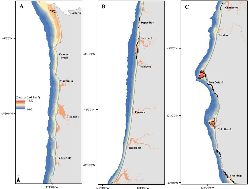
Fig. 1. Predicted sea otter densities along the outer coast and in estuaries of Oregon, USA, for the (A) north, (B) central, and (C)
south regions. Density values are visualized using natural breaks (Jenks) with 12 data classes. Core habitat areas are outlined in
black and transposed over high-density values
identify contiguous core habitat areas, which we 2.6. Human activities
delineated using the ‘Raster to Polygon’ tool in ESRIs
ArcGIS. For each resulting core habitat area, we We assessed the potential for interaction (i.e.
summed predicted densities to calculate total abun- resource competition with fisheries and human dis-
dance. We then excluded core habitat area polygons turbance to sea otters) between sea otters in Oregon
whose combined abundance was lower than a and 3 types of human activities: fisheries, non-recre-
threshold of 8 to identify core habitat areas likely to ational vessel traffic, and protected areas. We col-
support relatively high sea otter abundances. We lected logbook landings data for the 10 most recent
set this abundance threshold at 8 by (1) identifying fishing seasons for a few commercial and recre-
all core habitat areas at or near historical sea otter ational fisheries (Table 3). To protect fishermen con-
foraging locations (Simpson, Orford, and Blanco fidentiality, data do not include harvest from fishing
Reefs) from the first translocation (Jameson 1974), grounds where relatively few vessels were present.
and then (2) identifying the single core habitat area However, harvest data do represent the vast majority
with the lowest abundance at those historical forag- of fishery landings over this time period. We selected
ing locations, to represent or suggest a minimum fisheries for target species that (1) are commonly con-
viable population size. sumed by sea otters and likely to be consumed in166 Endang Species Res 44: 159–176, 2021
Table 3. Interaction potential between sea otters and human activities, including potential sources of disturbance, in Oregon,
USA. Data layer descriptions and sources provided. Direct overlap and proximity metrics represent how interaction potential
between sea otters and human activities were measured for each activity, while interaction level reports the calculated interac-
tion potential for those associated metrics. Any ratios reported under interaction level are the proportions of activity or habitat
spatial units (i.e. polygons, cells, lines) that interact with each other. NA: not applicable
Activity Data layer Spatial Value Direct Interaction Proximity Interaction
resolution units overlap metric level metric level
Fisheries Dungeness crab 2 nm cells Annual crab Activity Yes (2/40) % activity 9% (area)
(commercial)a (N = 40) removals overlap within 2 km
(2007−2017)
Red sea urchin Harvest area Annual pounds Activity Yes (9/13) % activity 67% (area)
(commercial)a polygons (N = 13) (2009−2018) overlap within 2 km
Abalone Harvest zone Total ind. Activity Yes (8/8) NA NA
(recreational)a lines (N = 8) (2008−2017) overlap
Disturbance Recreations 1600 m cells Presence % habitat 58% Habitat Yes (10/10)
within within 2 km
Commercial Lane polygons Presence % habitat 1% Habitat Yes (3/10)
shipping & tow within within 2 km
lanesc,d
Fishing portse Port points (N = 12) Presence NA NA Activity Yes (5/12)
within 2 km
Protected Marine Reserve Presence % habitat Activity Yes (2/5)
areas reservesf polygons (N = 5) within 2% within 2 km
a
Fishery logbook data (ODFW 2019). bNon-consumptive Ocean Recreation in Oregon (LaFranchi & Daugherty 2011).
c
Electronic Navigation Charts (NOAA 2012). dWashington Sea Grant (2007). eEcotrust (Hesselgrave et al. 2011). fMarine
Reserves Program (ODFW 2010)
Oregon (Ostfeld 1982), and (2) are valued by local 2.7. Interaction potential
economies and/or conservation and, therefore, pres-
ent an opportunity for resource competition (ODFW We assessed interaction potential between core
2017a, 2019). We identified ‘high-catch crabbing habitat areas and human activities by quantifying 2
grounds’ as areas having harvests that were 2 stan- interaction metrics: direct overlap and proximity
dard deviations above the mean of the log-trans- (Table 4). We measured the percent overlap be-
formed commercial Dungeness crab logbook data. tween human activities and core habitat areas as
We included recreational data on human-powered the proportion of the total abundance of sea otters
(i.e. kayaking, surfing, swimming, scuba, snorkeling, within core habitat areas that spatially overlapped
and skimboarding) and wildlife-viewing activities
reported through an opt-in internet survey where
Table 4. Description of metrics used to describe interaction
respondents identified the type and location of potential between core habitat areas and human activities in
coastal activities they participate in (LaFranchi & Oregon, USA
Daugherty 2011). Responses were spatially joined
and displayed in polygon planning units used in Ore- Interaction Unit Human
gon’s Territorial Sea Plan. We assessed potential metric activity
non-recreational vessel activity by combining com-
Direct overlap Activity within All,
mercial shipping lanes, tugboat tow lanes, and ports
habitat (Yes/No) except ports
that provide facilities for large ships and commercial
% habitat All,
fishing boats (Hesselgrave et al. 2011). We included 1
within activity except ports
additional port (Newport), which was missing from
Proximity Activity within 2 km All
this dataset, with known commercial fishing process-
of habitat (Yes/No)
ing facilities. We also assessed the 5 no-take marine
% activity (area) Fisheries only
reserves in Oregon (Redfish Rocks, Cape Perpetua, within 2 km of habitat (Dungeness crab,
Cape Falcon, Cascade Head, and Otter Rock) as pro- sea urchin)
tected areas.Kone et al.: Sea otter reintroduction in Oregon 167
with human activity polygons. We also quantified region (Fig. 2), but a smaller proportion of these
proximity between core habitat area polygons and grounds (2%; 6.18/252.42 km2) were within dispersal
human activities, reasoning that activities were likely distance for sea otters, than in the north (11%; 20.40/
to interact with sea otters if they occurred within 178.30 km2) or south (19%; 21/109.71 km2) regions.
2 km of core habitat areas, based on reported daily Commercial fishermen harvested red sea urchins
dispersal patterns (i.e. 1 to 2 km) of sea otters at from 13 harvest areas (Fig. 2), primarily in the south
all age and sex classes (Ralls et al. 1995). Proximity region (north: 29.82 km2; central: 21.39 km2; south:
measures were more appropriate than propor- 84.84 km2). Most harvest areas overlapped and/or
tional overlap for certain human activities such were proximate to core habitat areas (Table 3), but
as those with point locations (e.g. ports) or diffuse some harvest areas had a greater potential of inter-
activities. For fisheries, we highlighted potential acting with foraging sea otters than others. In fact, 5
interactions with relatively high-landing fishing harvest areas were completely (100% by area)
grounds. within 2 km of core habitat areas, including Orford,
All associated datasets and spatial layers are avail- Rogue, and Blanco Reefs, which had the highest total
able in an online public data repository (https:// landings (18 2324 , 10 1694 , and 40 613 pounds yr−1,
figshare.com/projects/Oregon_Sea_Otter_Carrying_ respectively), constituting 83% (3.2 × 10⁶ / 3.9 × 10⁶
Capacity_Kone_et_al_2020_/78075). pounds yr−1) of all red sea urchin annual landings
across the state. The other 2 harvest areas, Nellie’s
Cove and Mack Reef, only comprised approximately
3. RESULTS 3% (1.0 × 10⁴ / 3.9 × 10⁶ pounds yr−1) of all landings,
combined.
3.1. Carrying capacity and core habitat areas Abalone were harvested from 8 harvest zones in
Oregon, primarily in the south region. All harvest
We predicted a total abundance of 4538 (1742− zones overlapped with, and were proximate to, core
8976; 95% CI) sea otters at carrying capacity within habitat areas (Table 3). We found most abalone land-
outer coast and estuarine habitats of Oregon. We ings (91%; 1336/1467 individuals) came from just 2
predicted higher total abundance and average otter harvest zones, but only 1.4% (13/926 otters) of core
density in the south region on the outer coast. How- habitat areas occurred within these zones.
ever, within estuaries, we predicted slightly higher When we considered fisheries as a potential dis-
abundances in the central region (Table 5). We pre- turbance to sea otters, we found all core habitat
dicted higher abundances along the entire outer areas overlapped with either high-catch crabbing
coast (3781 otters) than in estuaries (757 otters). We grounds or red sea urchin harvest areas. In total,
identified 10 core habitat areas (Fig. 2), mostly in approximately 76% (699/926 otters) of core habitat
the south region (80% of habitats;
742/926 otters). Core habitat areas Table 5. Predicted total abundance and mean (x–) sea otter densities (km−2), with
had an average abundance of 93 otters 95% confidence interval (CI), for each region in Oregon, USA. Estuary densities
per polygon, ranging from 8 to 494 are identical due to uniform estuarine density parameter applied to all estuaries
otters.
Region Total Lower CI Upper CI Density Lower CI Upper CI
(area km2) abundance (95%) (95%) (x–) (95%) (95%)
3.2. Human activities Outer coast
North
All fisheries examined in this study (1079 km2) 1233 473 2439 1.83 0.70 3.61
either overlapped with, or were proxi- Central
(1175 km2) 997 383 1972 1.74 0.67 3.44
mate to, core habitat areas, but the South
interaction potential varied between (1005 km2) 1551 595 3068 2.45 0.94 4.84
fisheries. A small proportion of pri- Estuaries
mary Dungeness crabbing grounds, North
where 22% of crab are caught along (63 km2) 233 90 462 3.73 1.43 7.37
the coast, overlapped with and/or Central
(78 km2) 290 111 574 3.73 1.43 7.37
were proximate to core habitat areas
South
(Table 3). Most high-catch crabbing (63 km2) 234 90 462 3.73 1.43 7.37
grounds occurred within the central168 Endang Species Res 44: 159–176, 2021
Simpson
A 45°0'0"N B C Reef Charleston
Astoria
Depoe Bay
Bandon
46°0'0"N
43°0'0"N
Newport
Cannon
Beach
44°30'0"N
Blanco
Reef
Waldport
Orford Port Orford
Manzanita Reef
Tillamook
45°30'0"N 42°30'0"N
44°0'0"N Florence
Rogue
Reef
Gold Beach
Reedsport
Pacific City
43°30'0"N
Brookings
42°0'0"N
124°0'0"W 124°30'0"W 124°0'0"W 124°30'0"W
Fig. 2. Spatial location of predicted sea otter core habitat areas (green polygons) along the outer coast and the potential over-
lap with and proximity of these areas to high-catch crabbing grounds (blue hatched grid cells; data from 2007 to 2017), sea
urchin harvest areas (red hatched polygons; data from 2009 to 2018), fishing ports (yellow dots; data from 2011), and marine
reserves (turquoise polygons; data from 2010) across regions (A: north; B: central; C: south) in Oregon, USA
areas overlapped with fisheries. We did not in- ports, and tow lanes were scattered across all regions
clude abalone harvest zones in this estimate due throughout the study area (Fig. A1 in the Appen-
to lack of spatial resolution. dix). We found no overlap with tow lanes, but a
By area, most recreation (i.e. human-powered and small degree of overlap with commercial shipping
wildlife viewing) took place in the central region lanes (1% core habitat areas; 9/926 otters). Fishing
(45%; 606.25/1355.52 km2), relative to the north ports were located across the entire study area.
(26%; 357.78/1355.52 km2) and south (29%; 391.49/ When we considered potential disturbance from all
1355.52 km2) regions. While core habitat areas did non-recreational sources of potential vessel activity
not overlap entirely (58%; 536/926 otters) with recre- (i.e. fishing ports, commercial shipping lanes, and
ational activity, all core habitat areas did directly tow lanes) to core habitat areas, we found most core
overlap with recreational activity to some degree. habitat areas (N = 7) were proximate to some form of
Most of this overlap occurred in the south (68%; vessel activity. Importantly, all (2/2) core habitat
365/536 otters) and central (32%; 170/536 otters) areas in the central region, and most (5/6) in the
regions. Commercial shipping lanes were located south, could be disturbed by some form of vessel
primarily offshore but extend to the shoreline at 5 activity.Kone et al.: Sea otter reintroduction in Oregon 169 By combining all potential disturbances (i.e. fish- habitat. In the 1970s, sea otters were observed to rou- eries, recreation, shipping and tow lanes, ports), we tinely forage at Orford, Blanco, and Simpson Reefs found the vast majority (97%; 896/926 otters) of core along the southern coastline (Jameson 1974). Our habitat areas overlap with some form of disturbance. current results also suggest that these reefs represent Among regions, approximately 1% (13/896 otters), potentially important future habitats for sea otters, 19% (170/896 otters), and 80% (714/896 otters) of providing a total of 24 km2 of core habitat areas this potential direct disturbance occurred in the within 52 km of each other. We identified another north, central, and south regions, respectively. large core habitat area just south of Newport, OR Within regions, direct disturbance from the evalu- (21.12 km2; 133 otters). Together these findings sug- ated factors could affect approximately 85% (13/15 gest the southern coastline may be more suitable for otters), 100% (170/170 otters), and 96% (714/742 sea otters, based on habitat alone, with some poten- otters) of core habitat areas in the north, central, and tially important habitats along the central coastline, south regions, respectively. and little along the north coast. While our findings The marine reserves in Oregon were somewhat cannot conclusively address whether the 1970s failed evenly distributed within the study area, including sea otter translocation was due to lack of suitable Cape Falcon (32 km2; north region), Cascade Head habitat, they suggest this was probably not the case. (25 km2; central region) Otter Rock (3 km2; central Human interactions and disturbance have been sug- region), Cape Perpetua (36 km2; central region), and gested as a potential cause of the 1970s failed trans- Redfish Rocks (7 km2; south region). Two of these location effort (Jameson 1974). In the present study, marine reserves overlapped with, or were proximate we show that sea otters could interact with humans to, core habitat areas: Otter Rock and Redfish Rocks and potentially face disturbance from fisheries, recre- marine reserves. Two percent (19/926 otters) of core ation, and various sources of vessel activity (i.e. com- habitat areas overlapped with Otter Rock (
170                                     Endang Species Res 44: 159–176, 2021

may not be the case. If landings and efforts are not           Resource competition between sea otters and fish-
correlated, there may be other areas in our study           eries is a common concern across the sea otter range
area where sea otters may be disturbed by fishing           (Carswell et al. 2015). Our study directly addressed
activity.                                                   those concerns by assessing potential interactions
   Proximity to disturbance is an assessment of poten-      between sea otters, based on core habitat area distri-
tial disturbance to sea otters while foraging within        bution, and the Dungeness crab and red sea urchin
2 km of core habitat areas. Our disturbance proxim-         commercial fisheries in Oregon. We found very little
ity results should not be interpreted as the distance       spatial overlap between core habitat areas and crab-
between a sea otter and disturbance stimuli that elic-      bing grounds that produce the highest annual land-
its a behavioral or physiological response, but rather      ings in the commercial Dungeness crab fishery,
they should be considered as the areas of the marine        which is the most lucrative fishery in Oregon (ODFW
environment beyond core habitat areas where sea             2017a). Based on these results, we suspect sea otters
otters could come into direct contact with humans           and commercial crabbers may experience relatively
while foraging. We recognize sea otters are more            limited resource competition and interaction. Dunge-
likely to elicit a behavior response within 54 m of         ness crab is a soft-sediment species (Holsman et al.
human activities (Barrett 2019), but this distance esti-    2006), which likely explains the lack of spatial over-
mates the Euclidean distance between the observed           lap between important crabbing grounds and core
location of a sea otter and disturbance stimuli. Our        habitat areas. Many of these crabbing grounds occur
analysis is precautionary as it considers all potential     in areas where sea otters are predicted to be less
areas where sea otters may interact with humans             dense, and in offshore areas that are beyond the
given their dispersal potential (i.e. within 2 km).         diving capacity of sea otters (Bodkin et al. 2004). Sea
While foraging, sea otters can disperse further than        otters may interact with the commercial crab fishery
2 km (e.g. 4 km; Ralls et al. 1995, Tarjan & Tinker         in isolated areas, but we suspect they are unlikely to
2016), but we applied a 2 km threshold as a conser-         impact or compete with the entire fishery. One limi-
vative estimate given our use of a 4 km smoothing           tation of these crabbing−otter interpretations is that
window that already considers dispersal potential.          they only represent potential interactions with poten-
Therefore, we intended to avoid overestimating dis-         tial adult Dungeness crab population distribution,
persal, as this might unrealistically increase our dis-     inferred from fishery landings data. Juvenile Dunge-
turbance potential results.                                 ness crabs concentrate in relatively shallow habitats —
   Furthermore, our assessments assume all human            including intertidal zones and estuaries (Fernandez
activities disturb sea otters to the same degree and,       et al. 1993, Armstrong et al. 2003). If core habitat
therefore, are equally likely to reduce or limit popu-      areas spatially overlap with or are proximate to shal-
lation reestablishment. This assumption makes our           low habitats inhabited by juvenile crab populations,
disturbance results highly speculative as (1) we lack       sea otter predation on juvenile crabs could poten-
knowledge on the relative importance of various             tially reduce adult crab recruitment and eventually
forms of human disturbance on sea otter behavior            impact the commercial fishery. The results of our
and energetics and (2) research on the population-          study do not address this hypothetical scenario, so
level consequences of human disturbance on sea              more research on this potential impact is warranted.
otters is nascent. Most research has focused on recre-         In contrast with the minimal overlap with crabbing
ation due to the proximity of sea otters to ecotourists     grounds, we found a high degree of overlap between
(Curland 1997, Benham 2006), and distance from a            the red sea urchin and abalone fisheries and core
sea otter to a disturbance stimulus is a good predictor     habitat areas. This finding is perhaps not surprising
of behavior response probability (Barrett 2019).            given the similarities in habitat preferences of all 3
Given that proximity is a key factor, we expanded           species for rocky reefs (Tegner & Levin 1982, Kato &
our disturbance assessments to other forms of human         Schroeter 1985). Given the proximity of these high-
activities that are proximate to core habitat areas and     landing harvest areas to core habitat areas, these
may elicit similar behavioral and physiological re-         results suggest a high potential for interaction with,
sponses in sea otters as recreation. Given our assump-      and impacts from, sea otters for these fisheries.
tions, direct overlap may be a stronger indicator of        Importantly, sea otters are size-selective predators
potential disturbance and we recommend that fur-            that target larger individuals within prey populations
ther research should address the relative influence of      (Ostfeld 1982). Urchin fisheries also target large indi-
different types of human disturbance on sea otter           viduals, which is likely why there is no evidence of
behavior and energetics.                                    viable commercial red sea urchin fisheries occurring
Kone et al.: Sea otter reintroduction in Oregon                               171

within areas occupied by sea otters in other regions.         (i.e. sea urchins, abalone). Reduced kelp could limit
If sea otters are reintroduced to Oregon, it is highly        prey population size and quality (i.e. mass), which
likely Oregon could experience similar declines in            could limit otter densities. Kelp variability could also
large sea urchins, eventually making it difficult or          redistribute core habitat areas from where we have
impossible for a commercial urchin fishery to persist         predicted. This limitation highlights the important
in areas where sea otters have recovered. Managers            bottom-up processes that support sea otters and how
may therefore wish to consider alternative economic           environmental variability may impact sea otter abun-
opportunities for commercial urchin fishermen and             dance and distribution. Yet, through their strong top-
divers, specifically, before they decide whether to           down pressures, sea otters can help maintain eco-
proceed with a reintroduction effort. Similarly, abalone      system function and important habitats, such as kelp,
population reductions via sea otter predation could           by controlling herbivores, like sea urchins. Recently,
also threaten the viability of Oregon’s recreational          northern California (where sea otters have histori-
fishery or may even be a conservation concern, given          cally occurred, but do not currently) experienced a
current abalone population declines (ODFW 2017b).             90% reduction in canopy-forming bull kelp due to
However, it is worth noting that abalone in other             climatic and biological stressors, with purple urchin
regions have been found to persist within cryptic             grazing being a major contributor (Rogers-Bennett et
habitats, sometimes at elevated densities, in areas           al. 2019). To date, Oregon has only experienced
having high density sea otter populations (Lee et al.         some kelp cover reductions in isolated locations,
2016, Raimondi et al. 2015).                                  nowhere near the extent observed in northern Cali-
   Marine protected areas represent one possible ap-          fornia. Yet, if these events continue to unfold in Ore-
proach to minimizing human−sea otter interactions             gon, reintroducing sea otters might help limit large-
that may lead to disturbance or resource competition.         scale losses of kelp forests like that which has
Unfortunately, our analyses suggest that sea otters           occurred in northern California. Despite these limita-
may be afforded little protection by current marine           tions, we feel our extrapolation of sea otter densities
reserves in Oregon due to limited spatial overlap             associated with key habitat variables from California
between core habitat areas and reserves. Protecting           to Oregon is appropriate given relative geographic
the types of habitats important to sea otters was un-         proximity, data availability, and application of this
likely to have been a priority for managers while             novel approach. To address this limitation, however,
establishing the Oregon marine reserves, which could          future analyses could determine sea otter density
explain these findings. Several other protected areas         and habitat functional relationships in other locations
exist along the Oregon coast (i.e. marine gardens,            within the current range of sea otters (e.g. Washing-
limited-access protected areas, and national wildlife         ton, Alaska, British Columbia) to assess how repre-
refuges), but we did not assess these protected areas         sentative the California data may be of Oregon.
as they are not fully protected, and monitoring and              A second caveat to our results relates to the pro-
enforcement are limited. Even if these protected              jected abundances in estuaries. The densities of estu-
areas only prohibit some human activities some of             arine sea otter populations predicted by the CA
the time, that exclusion could help protect and pre-          model are informed by the few currently occupied
serve potentially important sea otter habitat and             estuaries in California, specifically Morro Bay and
could be investigated in future research.                     Elkhorn Slough. The former estuary supports a fairly
   The results of our study come with a few caveats           low abundance of otters, while the latter (Elkhorn
and limitations. First, this study is an extension and        Slough) supports a very high abundance, apparently
an extrapolation of how habitats support sea otter            sustained by an abundant and productive prey base
populations in California, but it is uncertain whether        (Kvitek & Oliver 1988). The contrast in abundance
Oregon habitats, especially kelp canopies, will sup-          between the 2 California estuaries leads to a high
port similar equilibrium sea otter densities as in Cal-       degree of uncertainty in our model estimate for estu-
ifornia. The CA model indicates that the presence of          arine habitats. Extrapolation of the model to Oregon
kelp canopy is associated with higher sea otter den-          estuaries effectively projects an average of the Morro
sities; however, those results are likely driven prima-       Bay and Elkhorn Slough equilibrium densities, with
rily by giant kelp Macrocystis pyrifera, a species            very large associated standard error. While this ap-
which is more persistent (Foster & Schiel 1985) than          proach may be reasonable as a first pass approach,
Oregon’s bull kelp, which experiences intra- and              further research is needed to elucidate the potential
inter-annual variability (Springer et al. 2007). Kelp         of Oregon estuaries to support thriving sea otter
provides an important food resource for otter prey            populations.
172                                     Endang Species Res 44: 159–176, 2021

   A third limitation of our analyses is that we only       previously discussed, habitat and biotic features can
identified core habitat area and potential human            shift over time due to any number of forces (e.g. cli-
interactions on the outer coast, not within estuaries       mate change, ocean acidification, etc.). Humans may
and along shorelines. Our findings therefore do not         redistribute their activities, such as fisheries and
reflect the potential role estuaries and shorelines         reserves, in response to these ecological shifts, and
may play in supporting future sea otter populations,        so the patterns of potential interaction presented
including providing additional foraging habitat and         here may not hold under such changes.
resting areas to haul out (despite this behavior being
rare), nor do they capture the potential for human−
sea otter interactions in estuaries. Sea otters occur in                       5. CONCLUSIONS
Elkhorn Slough, an estuary in California, with high
population density supported by locally abundant               Reintroductions are a well recognized strategy to
clam populations (Kvitek & Oliver 1988, Maldini et          augment the recovery of at-risk species (Clark &
al. 2012, Hughes et al. 2013, Eby et al. 2017). There is    Westrum 1989, Seddon et al. 2007). A sea otter re-
also evidence that other California estuaries (e.g. San     introduction to Oregon could reestablish this once
Francisco Bay, Drakes Estero, and Morro Bay) were           native species and help sea otters recover from previ-
historically occupied by sea otters, based on archaeo-      ous human exploitation. However, given the risk of
logical remains discovered in Native American shell         another failed reintroduction effort and lack of infor-
middens and anecdotal accounts of sea otter estuarine       mation to explain that failure, managers have not yet
habitat use (Schenck 1926, Odgen 1941, Broughton            decided whether they will proceed with a reintroduc-
1999, Jones et al. 2011, Hughes et al. 2019). The           tion. To facilitate the decision, we have attempted to
potential for California estuaries as future sea otter      address some of the common uncertainties associ-
habitat has recently been considered (Hughes et al.         ated with species reintroductions, including habitat
2019). Sea otters may also thrive in estuaries along        suitability. Our analyses indirectly address some of
the Oregon coast, with relative prey availability           the hypotheses for the cause of failure of the previous
likely acting as the primary determinant of popula-         translocation effort; for example, our results are not
tion potential. Many Oregon estuaries do contain            consistent with the ‘lack of suitable habitat’ hypothe-
populations of potential sea otter prey species, par-       sis, suggesting instead that the available habitat
ticularly bay clams and Dungeness crabs. In fact, in        could support a population of > 4500 sea otters. Our
some of the estuaries identified by our model (Alsea        study also identified areas of particularly high den-
Bay, Coos Bay, Netarts Bay, Siletz Bay, Tillamook           sity, and potential interactions with human activities.
Bay, Yaquina Bay), bay clam populations have been           Managers could use this information to set reason-
identified (Ainsworth et al. 2014). To better under-        able population recovery targets that factor in both
stand the potential for Oregon estuaries to play a role     ecological and socioeconomic considerations. Lastly,
in supporting a resident sea otter population, future       we have investigated the potential to reintroduce sea
research should investigate prey availability, and          otters to Oregon from a bottom-up perspective; mov-
human use and presence within and/or near poten-            ing forward, an important next step will be to con-
tially important estuaries.                                 sider how reestablishing sea otters could change the
   A final caveat is that our examination of potential      environment via top-down processes. Reintroducing
human−sea otter interactions in Oregon lacks spatial        sea otters could result in negative effects to certain
and temporal resolution. Carrying capacity predic-          commercial fisheries but could also lead to positive
tions were calculated using a finer spatial resolution      outcomes such as restored kelp habitats and ecologi-
than was available for most of the human activities,        cal resilience that supports fisheries and tourism
specifically commercial Dungeness crab cells, aba-          operations. As managers consider whether to pro-
lone harvest areas, and recreation planning units.          ceed with a reintroduction, monitoring will be key to
The available data indicate approximately where             understanding how these bottom-up and top-down
those activities are located but lack spatial precision     processes will play out, providing insight into the
and are thus representative of very general patterns.       trade-offs associated with each process, and assessing
Additionally, these interpretations are temporally          the ultimate success of the reintroduction effort.
static. We only considered where core habitat areas
are located relative to current human activities, and
                                                            Acknowledgements. We thank ODFW’s Marine Resources
did not consider seasonal patterns, or the time course      Program and fishery managers for collecting and synthesiz-
from reintroduction to equilibrium abundance. As            ing the fisheries logbook data, specifically E. Perotti, J.
You can also read