Integrated Structure-Control Design of a Bipedal Robot Based on Passive Dynamic Walking
←
→
Page content transcription
If your browser does not render page correctly, please read the page content below
mathematics

Article
Integrated Structure-Control Design of a Bipedal Robot Based
on Passive Dynamic Walking
Josué Nathán Martínez-Castelán †                   and Miguel Gabriel Villarreal-Cervantes *,†

                                          Mecatronic Section, Postgraduate Department, Instituto Politécnico Nacional, CIDETEC,
                                          Mexico City 07700, Mexico; jmartinezc1317@alumno.ipn.mx
                                          * Correspondence: mvillarrealc@ipn.mx
                                          † These authors contributed equally to this work.

                                          Abstract: The design of bipedal robots is generally fulfilled through considering a sequential design
                                          approach, where a synergistic relationship between its structure and control features is not promoted.
                                          Hence, a novel integrated structure-control design approach is proposed to simultaneously obtain
                                          the optimal structural description, the torque magnitudes, and the on/off time intervals for the
                                          control signal input of a semi-passive bipedal robot. The proposed approach takes advantage of
                                          the natural dynamics of the system and the control signal activation/deactivation for generating
                                          stable gait cycles with minimum energy consumption. Consequently, the passive features of the
                                          semi-passive bipedal robot are included in the integrated structure-control design process through
                                          evaluating the system behavior along consecutive passive and semi-passive walking stages. Then,
                                          the proposed design approach is formulated as a nonlinear discontinuous dynamic optimization
                                          problem, where the solution search is carried out using the differential evolution algorithm due to the
                                discontinuities of the semi-passive bipedal robot dynamics. The results of the proposal are compared
                                   with those obtained by a sequential design process. The integrated structure-control design achieves
Citation: Martínez-Castelán, J.N.;        a reduction of 63.55% in the value of the performance function related to the synergy between the
Villarreal-Cervantes, M.G. Integrated     walking capability and energetic efficiency, with a reduction in the activation of the control and its
Structure-Control Design of a Bipedal     magnitude of 95.41%.
Robot Based on Passive Dynamic
Walking. Mathematics 2021, 9, 1482.       Keywords: structure-control design; optimization; passive bipedal walker; bipedal robots; differen-
https://doi.org/10.3390/math9131482
                                          tial evolution

Academic Editors: Theodore E. Simos
and Charampos Tsitouras

                                          1. Introduction
Received: 26 May 2021
Accepted: 19 June 2021
                                                Artificial bipedal walkers are systems that can walk due to the alternated execution of
Published: 24 June 2021
                                          single and double support phases of their legs. Then, the single support or swing phase
                                          is defined as the locomotion phase where only one foot is on the ground; conversely, the
Publisher’s Note: MDPI stays neutral
                                          double support phase is described when both feet of the system is in contact with the
with regard to jurisdictional claims in
                                          walking surface [1]. There exist three types of bipedal machines that can develop stable
published maps and institutional affil-   gait cycles [2]. The first type studies the fully actuated bipedal robots that are mechatronic
iations.                                  systems where a precise joint-angle control is required to produce bipedal locomotion.
                                          This approach has reached impressive results mainly associated with the control design
                                          of humanoid robots, for instance, the navigation and interaction of the ASIMO robot [3],
                                          the walking on a low friction floor of the humanoid robot HRP-3 [4], the walking on
Copyright: © 2021 by the authors.
                                          large obstacles of the humanoid robot HRP-2 [5], among others. Nevertheless, the high-
Licensee MDPI, Basel, Switzerland.
                                          frequency response of actuators and real-time control computation cause that these robots
This article is an open access article
                                          are energetically inefficient [6]. The second type addresses the passive bipedal walkers
distributed under the terms and           that can achieve stable gait cycles without any control input. Tad McGeer demonstrated
conditions of the Creative Commons        in his seminal work [7] the importance of mechanical structure in bipedal machines. His
Attribution (CC BY) license (https://     work showed that a purely passive walker can develop stable gait cycles when the system
creativecommons.org/licenses/by/          is located over an inclined surface. Despite the energetic efficiency of this type of system,
4.0/).                                    they are not versatile since it is not possible to actively modify its gait indicators, such as

Mathematics 2021, 9, 1482. https://doi.org/10.3390/math9131482                                         https://www.mdpi.com/journal/mathematics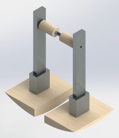
Mathematics 2021, 9, 1482                                                                                            2 of 26

                            speed or stride length; also, an inclined surface is always needed to generate the system’s
                            movement. The third type is the bipedal robots based on passive dynamic walking, which
                            combine the advantages of actuated robots and passive walkers; thus, this type of system
                            considers the inertial properties provided by the robot mechanical structure to promote
                            appropriate bipedal locomotion using simpler and energetically efficient control strategies.
                            Relevant examples of these bipedal systems are described in [8,9], where in both cases, a
                            finite-state machine based on the walking process phases was implemented for actuating
                            the robot joints; these works demonstrated that artificial bipedal machines can reproduce
                            human-like walking using a simple on/off control signal.
                                  Presently, most studies about bipedal robots are mainly focused on two research
                            trends. The first one addresses the proposal of novel control schemes. However, they
                            are commonly implemented in robotic platforms already built. This approach produced
                            suitable results generating stable gait cycles. For instance, in bipedal robots based on
                            passive dynamic walking, using a nonlinear control based on tracking of the mechanical
                            energy [10], with a simple controller and the use of potential energy-conserving orbit [11],
                            with active control strategies applied to a partially actuated version of a 3D passive dynamic
                            walker [12], and other strategies reported in [13] such as the use of zero moment point
                            controllers and balance control based on foot placement. The second research trend studies
                            the optimization-based structural design of bipedal systems, where the problem of finding
                            the optimal structure parameters for different types of walking systems was proposed. For
                            instance, in the design of the passive bipedal walker leg that performs limit cycles in both
                            the frontal and sagittal planes [14], in the design of an eight-bar mechanism to fulfill the
                            desired locomotion task with a minimum force transmission during the stance phase [15,16],
                            in the design of Stephenson III six-bar mechanism for tracking of a gait trajectory [17] and in
                            the optimal mass distribution for passive dynamic biped robot [18]. Although both research
                            trends have shown their own advantages, the trade-off between the natural dynamics of
                            the structure and the control signal features related to the walking performance has not
                            been addressed. Consequently, an integrated mechatronic design technique is proposed
                            in this paper to explore the relationship between both design domains (structure and
                            control) of bipedal robots for improving their overall performance to maintain a limit cycle
                            dynamic response.
                                  The highlights of considering structural and control requirements into a unified de-
                            sign stage were explored in [19–23]. One of the first integrated design applications was
                            published in [19], where a unified design process obtained optimal structural and control
                            parameters of a flexible spacecraft. The design of a high-speed flexible robot arm was
                            developed in [20]. In this work, the stability properties of the robotic arm were improved
                            by simultaneously considering the mass and stiffness distributions of its links and the
                            placement of actuators and sensors. The derivation of controllers with optimal whiplash
                            nature that account the interactions of the structural dynamics of flexible space robots
                            is presented in [23] with the use of variational approach [24]. The main benefit of that
                            approach is that it can develop an in-plane maneuver with minimum time without residual
                            vibration. An integrated control and structural design approach for deployable space anten-
                            nas was carried out in [21]; here, the design tasks involved the coupling among the antenna
                            structure, deployment trajectory, and control system through solving a multi-objective
                            optimization problem. A synergistic optimal design of a planar underactuated manipula-
                            tor robot was addressed in [22], where trajectory tracking tasks were improved through
                            reducing mass and elastic deformations of the robot’s links, in addition, to minimize the
                            actuation forces. In the case of bipedal robots, integrated design techniques have been
                            applied only for fully actuated systems. A design process of a fully actuated bipedal robot
                            that simultaneously considers its mass distribution and its controller signal was carried
                            out in [25]; here, a genetic algorithm (GA) was implemented to tune a neural controller
                            and to find the appropriate mass distribution for a bipedal walker with fixed-length legs
                            and knee joints. Similar work was proposed in [26], where the morphology and control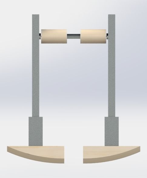
Mathematics 2021, 9, 1482                                                                                            3 of 26

                            of a pseudo-passive bipedal robot (i.e., all joints are continuously actuated as oscillators)
                            were coupled in the same design procedure; in this approach, also a GA was used.
                                  On the other hand, despite the integrated design problems that gradient-based opti-
                            mization techniques can address, the highly nonlinear properties of mechatronic systems
                            propitiate that its solutions search converges towards a local optimum. Therefore, in recent
                            years global optimization methods as meta-heuristic algorithms have been preferred for
                            solving complex mechatronic design problems. The performance of these algorithms in
                            searching solutions was verified in many mechatronic design cases [27–31]. The simul-
                            taneous design of a gravity balanced two-link planar manipulator robot was carried out
                            in [27]; here, the evolution strategy (µ + λ)-ES was implemented with regards of obtaining
                            its optimal structure design and the nonlinear gain PD controller parameters in the same
                            optimization process. A concurrent design methodology for the mechatronic design of
                            a pinion-rack continuously variable transmission was implemented in [28]; this design
                            problem was solved through mathematical programming and evolutionary methods, vali-
                            dating the global search capabilities of the evolutionary one. A robust integrated design
                            approach was proposed in [29]. The design of a parallel robot and its controller was
                            addressed as a multi-objective optimization problem that minimizes the sensitivity of its
                            design objectives with respect to uncertain parameters as end-effector payload changes;
                            this design problem was solved using the DE algorithm. A problem of determining optimal
                            geometric parameters and PID controller gains for a parallelogram linkage robot was
                            exposed in [30]. The solution to this design problem was achieved using an estimation of
                            distribution algorithm. Lastly, an exhaustive exploitation mechanism for DE algorithm and
                            a multi-objective structure and control design problem were presented in [31]. This work
                            dealt with the design of a serial-parallel manipulator where the exploitation mechanism
                            was implemented with the aim of finding better trade-offs in the structure and control
                            design domains.
                                  In the works related to the simultaneous design of bipedal robots [25,26], two relevant
                            design considerations are not addressed: First, the purely passive dynamic behavior of the
                            bipedal structure was not explored with the purpose of influencing the integrated design
                            process. Thus, by exploiting the inertial properties of the structural elements and the passive
                            dynamic walking capacity of a bipedal robot, the overall performance for maintaining the
                            system’s dynamic behavior into a limit cycle can be improved by proposing a control signal
                            that is not continuously activated. Second, with respect to the structural parametrization,
                            since previous works only studied the mass distribution of the robot links, the full physical
                            description of the robot requires solving an additional optimization problem to obtain
                            each structural component’s geometric and material characteristics. On the other hand, in
                            these previous works, the proposed controllers imply a full actuation of the system because
                            control signals are applied continuously along with the gait development.
                                  Hence, in this work, the integrated structure-control (S-C) design of a bipedal robot
                            based on dynamic walking known as Semi-Passive Bipedal Robot (SPBR) is proposed. This
                            approach takes advantage of the natural dynamic properties and a semi-passive control
                            strategy to promote the convergence of the system’s dynamic behavior towards a limit cycle.
                            The design proposal is formulated as a nonlinear discontinuous dynamic optimization
                            problem, where the objective function is focused on achieving a periodic motion of the
                            SPBR along with two consecutive passive (inclined ground) and semi-passive (leveled
                            ground) walking scenarios with a minimal control effort. The considered design variables
                            include the geometric description of each structural element, its material assignment, the
                            control input parameters, and a set of walking conditions variables that externally modify
                            the dynamic behavior of the SPBR. The results are validated by comparing the obtained
                            integrated design with an SPBR derived from a sequential design process.
                                  Due to gradient-based optimization techniques cannot efficiently handle system dis-
                            continuities, the meta-heuristic optimization method is implemented. Based on the suc-
                            cessful use of the DE algorithm in solving integrated design problems of mechatronic
                            systems such as in pinion-rack continuously variable transmissions [28], in five-bar parallel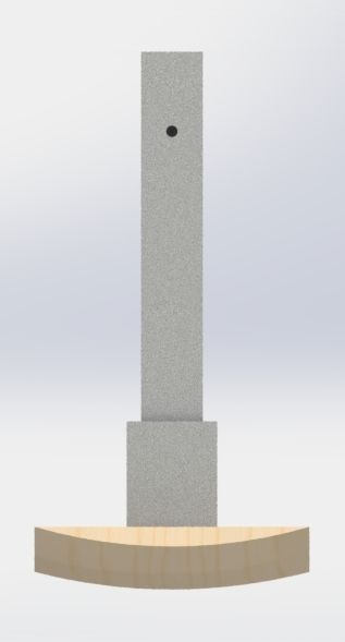
Mathematics 2021, 9, 1482                                                                                              4 of 26

                            robots [32,33] and in digital displacement machine [34], the variant DE/rand/1/bin [35]
                            with a constraint handling mechanism [36] is applied in the proposal with the aim of
                            guiding the solution search towards the feasible design region. Furthermore, because the
                            material assignment of structural elements is related to a finite set of available materials, a
                            discrete variable handling is incorporated into the DE algorithm [37].
                                 The rest of the paper is organized as follows: The dynamic model of the SPBR and the
                            semi-passive control strategy are presented in Section 2. The formulation of the integrated
                            S-C design problem is established in Section 3, where the objective function, design vector,
                            and constraints are described. The results and a comparative analysis between the proposal
                            and a sequential design process are presented in Section 4. Lastly, the conclusions are
                            drawn in Section 5 The descriptions of all the used symbols in this article can be seen in
                            Appendix A.

                            2. System Description
                                 With the aim of formulating the integrated S-C design proposal, the physical impli-
                            cations related to the dynamic behavior of the SPBR must be established. Hence, in the
                            following subsections, the dynamic model of the system and the proposed control strategy
                            are presented.

                            2.1. SPBR Dynamic Model
                                  To describe the dynamic behavior of the SPBR, some assumptions are defined [12]:
                            (i) The SPBR is composed of two rigid links as legs, curved feet, and one frictionless joint
                            placed in the hip. (ii) The motion of the SPBR takes into account frontal and sagittal plane
                            dynamic behaviors (no walking direction changes are studied). (iii) The frontal plane
                            dynamics is related to an oscillatory motion, which implies that the system rocks side to
                            side for avoiding premature contact between the swing leg and the walking surface. (iv)
                            The sagittal plane dynamics describes the stride of the system; hence, linear displacement
                            of the SPBR is constrained to this plane. (v) The interaction between feet and walking
                            surface neglects slipping and friction, and, the swing leg collisions are fully inelastic.
                                  The kinematic parameters of the sagittal plane model are the foot rolling radius Rs and
                            the lengths b and d, as Figure 1. depicts. With respect to sagittal plane dynamic parameters,
                            the system is described by the mass msag , the center of mass CMsag , and the inertia moment
                            Isag of each leg of the SPBR. In the case of the SPBR frontal plane model, the kinematic
                            parameters which describe the system are the length a, the separation angle φ, and the
                            foot rolling radius R f , as Figure 2 shows. Moreover, the considered dynamic parameters
                            are the mass m f ro , the link mass center CM f ro , and the inertia moment of both SPBR legs
                            considering them as a single link.
                                  A hybrid dynamic model describes the frontal and sagittal plane movements of the
                            SPBR. Thus, each one of these movements is modeled by a nonlinear continuous function
                            and a nonlinear discrete function. The nonlinear continuous function is associated with
                            the single support phase of the bipedal gait and describes the movement of the SPBR that
                            occurs between two consecutive collision instants k ς . Hence, in this phase, the movement is
                            modeled from the instant when the swing leg leaves the ground (after collision instant k ς )
                            until the instant before it collides, and hence, a walking step finishes (before collision instant
                            k ς + 1). The subscript ς ∈ { f , s} indicates the SPBR plane in which collision is considered,
                            assigning ς = f and ς = s for frontal and sagittal plane, respectively. The nonlinear discrete
                            function is related to the double support phase, which models the collision event associated
                            with the gait cycle transition. This function describes the velocity transfer between legs
                            when an impact happens; then, after the swing leg collides with the ground at instant
                            k ς + 1, the current role of each leg (determined at collision instant k ς ) is interchanged and
                            the stance leg converts into swing leg and vice versa.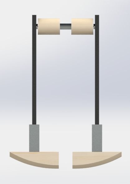
Mathematics 2021, 9, 1482                                                                                                 5 of 26

                                                        d

                                                            b

                                      msag
                                      Isag

                                                   Rs
                                    θsw                         θst      y

                                                                              x


                            Figure 1. Sagittal plane configuration of SPBR in single support phase.

                            2.1.1. Single Support Phase
                                  The dynamic response associated with the single support phase of the frontal and sagit-
                            tal plane is modeled by the Euler-Lagrange method [38] and its closed form is expressed as:

                                                   Mσ qη q¨η + Cσ qη , q˙η q˙η + Gσ qη = Φσ (t)

                                                                                                                      (1)

                            where Mσ qη is the positive semi-definite symmetric
                                                                                     inertia matrix, Cσ qη , q˙η is the
                            centrifugal and Coriolis force    o and Gσ qη is the vector of gravitational forces of the
                                                       n matrix
                            SPBR. Additionally, qη ∈ q f , qs indicates the considered system states for frontal and
                            sagittal plane, respectively, and Φσ (t) is the control strategy called in this paper as semi-
                            passive control one and is described in Section 2.1.3. The subscript σ ∈ {ss, rm, f c} assigns
                            the evaluated dynamic behavior in the single support phase. In the case of the single
                            support phase of the sagittal plane, σ = ss is assigned in (1); furthermore, the generalized
                            coordinate vector is established as qη =s = [θst (t), θsw (t)] T , where the subscripts refers to the
                            current role of the leg; thus, the subscript sw is assigned to the swing leg and the subscript st
                            to the stance leg. With respect to the single support phase of the frontal plane, the system’s
                            behavior is described by two dynamic conditions that depend on the angular position θ f
                            of the SPBR. Considering Figure 2a, the first condition is presented when θ f > φ; here,
                            qη = f = θ f (t) and σ = rm are set in (1) to define a rolling movement caused by the foot
                            radius R f . The second condition models the system as a fixed kinematic chain and occurs
                            when θ f ≤ φ (see Figure 2b); this means that the stance leg rotates around the inner foot
                            edge. For this second condition σ = f c is assigned in (1). For more details about single
                            support phase model, see Appendix B of [14].
Mathematics 2021, 9, 1482                                                                                      6 of 26

                                                                             a
                                                                 f

                                                    m fro
                                                    I fro

                                                                Rf
                               y

                                   x
                                                                     (a) θ f > φ

                                                                                   a

                                                                                    m fro
                                                                                    I fro


                                                                                                 Rf   y
                                                                                            f
                                                                                                          x

                                                      y

                                                            x
                                                                     (b) θ f ≤ φ

                            Figure 2. Frontal plane configuration of SPBR in single support phase.

                            2.1.2. Double Support Phase
                                 The swing leg collision (transition event) is described by discrete equations which
                            relate the SPBR states just before and just after the swing leg collides with the walking
                            surface. According to [39], the pre-impact and post-impact configurations of the system,
Mathematics 2021, 9, 1482 7 of 26
can be determined by q+ − 2×2 is an anti-symmetric matrix with unit
η = Wqη , where W ∈ R
elements and q+ − 2
η , qη ∈ R . The superscripts + and − in the system states indicate the SPBR
configuration after and before collision instants, respectively. Therefore, the principle of
conservation of angular momentum is used to determine the velocity transfer between
both legs at collision instant k ς , ∀ ς ∈ { f , s} through the expression:
−
−
Ω+
+
k ς qη q̇η = Ωk ς qη q̇η (2)
This equation is evaluated in the sagittal and frontal plane collisions and is only
computed once per transition event. For the detailed description of the double support
phase equations, see Appendix B of [14].
2.1.3. Semi-Passive Control Strategy
The proposed control strategy called semi-passive control one is focused on showing
that the SPBR design can improve its walking performance by considering the passive
dynamics of the system into the integrated design approach. Thus, to explore the influence
of the robot’s passive properties into design tasks, the system’s dynamic behavior is tested
over two consecutive walking scenarios known as Passive Walking Stage (PWS) and
Semi-Passive Walking Stage (SPWS). The number of evaluated collisions determines each
p sp
walking stage, assigning k s for the collisions in the PWS and k s for the collisions in the
SPWS. These scenarios are only defined for the sagittal plane dynamics and their evaluation
is carried out along the sagittal plane walking time t̂s , from t̂s = 0 to t̂s = tsag as Figure 3
shows. In the following, both walking scenarios are explained.
First, in the PWS, the SPBR takes advantage of its structural features and gravity force
to generate stable gait cycles without any control input when it is located over a surface
with an inclination angle γ 6= 0. Thus, the passive dynamic behavior of the system is
characterized by the gait cycles which occur from collision instant k s = 1 until the last
p
collision of the PWS (i.e., k s = k s ).
Second, in the SPWS, the surface is leveled at γ = 0, and the control signal is suitably
activated/deactivated based on a finite-state machine, which permits the system to con-
serve its periodic movement. This scenario evaluates the system behavior from collision
p p sp
instant k s = k s + 1 until the last considered collision k s = k s + k s .
Therefore, the gait characteristics derived from the PWS are used to develop gait cycles
in the SPWS with regards to promoting a synergistic relationship between the structural
properties and the control design features. Then, the sagittal plane dynamic behavior is
p sp
associated with the gait cycle periods Tsag and Tsag , both related to the periodic movements
of the system in the PWS and SPWS, respectively.
On the other hand, it is assumed that the frontal plane motion is purely passive (i.e.,
only influenced by gravity and its initial angular position θ f i ) and is characterized by its
oscillation period T f ro . It is important to remark that the single support phase time interval
p
ts of SPWS gait cycles is determined by the half of the PWS gait period (i.e., ts = Tsag /2).
Considering that the controller is only defined along the SPWS, the finite-state machine
determines the control signal mode (activated/deactivated) for each single support phase
which occur in this walking scenario. There are taken into account two controller states
per each single support phase time interval ts that happens after each collision instant
k s . The first state S1 is related to the control signal deactivation, where the movement is
only influenced by the natural dynamics of the SPBR structure; thus, along the deactivated
p
control time interval ∆tks , the control input is set as Φσ=ss (t) = [0, 0] T . In the case of
the second state S2, an external torque Φσ=ss (t) = [0, τks ] T , τks 6= 0 is applied along the
activated control time interval ∆tuks until the single support phase finishes. Hence, the
control signal is parameterized for each single support phase in the SPWS by its torque
magnitude τks and the time interval in which the control signal is activated ∆tuks , as can be
seen in Figure 3. Moreover, the considered control signal is applied on the hip joint and
only actuates the swing leg of the SPBR as is expressed in (3).Mathematics 2021, 9, 1482 8 of 26
(
[0, τks ] T if k s ∈ SPWS, ts ∈ ∆tuks
Φσ=ss (t) = (3)
[0, 0] T if k s ∈ PWS
Passive Walking Stage Semi-Passive Walking Stage
(PWS) (SPWS)
τ ks
θsw Semi-passive control parameters
θst θsw
(Single support phase)
θst ks ks +1
ts
p u
t k t
s s
τ ks=0 τ ks=0
S1 S2
p
Tsag =0 =0
p p sp
p
ks=ks +1 ks=ks +ks
ks=1 ks=2 sp
ks=ks Tsag /2
sp
ts=tsag
ts p sp
tc,ks=1 tc,ks=2 tc,ks=ks+ks
ts=0 ts=tsag
Figure 3. Walking stages of SPBR.
3. Integrated Structure-Control Design Problem
The objective of formulating the integrated S-C design problem of the SPBR is to
exploit its natural dynamic properties to find the optimal structural parameters and the
activated/deactivated control signal features that assure a periodic motion along the SPWS.
Thus, the PWS is implemented as a learning phase, where the obtained dynamic behavior
is taken as a reference for finding the required control parameters related to the SPWS
development. Therefore, the performance of the integrated S-C design approach can be
benefited by assuring that the SPBR shares its passive gait characteristics along with both
walking scenarios.
3.1. Objective Function
The formulation of the objective function is associated with two general design re-
quirements. The first one is related to the walking capability of the system and implies the
achievement of a synchronized periodic movement in the frontal and sagittal plane of the
SPBR. In the case of the second requirement, it is proposed that the system must develop
its gait cycles along the SPWS with minimum energy consumption.
3.1.1. Walking Capability Design Objective
The walking capability is related to the dynamic coupling of the frontal and sagittal
plane behaviors of the SPBR. This coupling is established to promote a periodic movement
that permits the gait cycle’s development. According to [14], the movement periodicity can
be promoted by minimizing the differences among the system state values of consecutive
transition events. Hence, the double support phases of the frontal and sagittal plane areMathematics 2021, 9, 1482 9 of 26
established as Poincaré Sections to evaluate a cyclic behavior of the system along with
the PWS and SPWS. Consequently, if the SPBR develops a periodic motion, its state-space
trajectories must not diverge and stay close to each other. Thus, the Poincaré Map is
expressed as:
qη,kς = Qς qη,kς −1 ∀ η, ς ∈ { f , s} (4)
where Qς is the Poincaré Section associated with the double support phase of each SPBR
plane, assigning ς = f and ς = s for the frontal and sagittal plane mappings, respectively.
In (4), the system states qη of frontal and sagittal dynamic models are evaluated just after a
transition happens. Then, the walking capability is promoted by minimizing the differences
among the frontal and sagittal plane Poincaré mappings of the SPBR through (5). This
expression evaluates the Poincaré mappings that happen in the dynamics simulation time
tc of each SPBR plane.
J1 = µ f Ψ f + µs1 Ψs1 + µs2 Ψs2 (5)
where Ψ f , Ψs1 and Ψs2 ∈ R are:
klast
f 2
Ψf = ∑ θ̇ f tc,k f − Q f θ̇ f tc,k f −1 (6)
k f =2
p
ks
∑ ∑
2
Ψ s1 = θq (tc,ks ) − Qs θq (tc,ks −1 )
k s =2 q={st,sw}
p sp
k s +k s 2
+ ∑p ∑ θq tc,k p − Qs θq (tc,ks )
s
(7)
k s =k s q={st,sw}
p
ks 2
Ψ s2 = ∑ ∑ θ̇q (tc,ks ) − Qs θ̇q (tc,ks −1 )
k s =2 q={st,sw}
p sp
k s +k s 2
+ ∑p ∑ θ̇q tc,k p − Qs θ̇q (tc,ks )
s
(8)
k s =k s q={st,sw}
In (6) the differences of Poincaré mapping values associated with the frontal plane
angular velocity are measured for the collision instants k f = 1, ..., klast
f which occur in
the frontal plane walking time t̂ f , from t̂ f = 0 to t̂ f = t f ro . In this case, klast
f indicates
the last collision that happens in the frontal plane walking time t̂ f . Considering that the
frontal plane dynamic behavior is depicted by a back-and-forth motion, it is assumed that
its transition events always occur at θ f = 0 (i.e., when both feet are instantly in contact
with the ground and the symmetry axis of the SPBR is perpendicular to it). Consequently,
only angular velocity is taken into account for convergence checking. In a similar manner
(7) and (8) are related to the differences of angular position and angular velocity of the
SPBR in the sagittal plane, respectively. In this case, both equations are divided into two
terms that evaluate the Poincaré mapping values of the PWS and SPWS consecutively.
Hence, to consider the passive performance of the SPBR into the SPWS, the states of all
collisions that occur in the SPWS are compared to the states of the last collision of the PWS
to maintain a passive influenced behavior. Additionally, the weighting factors µ f , µs1 and
µs2 are established to scalarize each term of (5).
3.1.2. Energetic Efficiency Design Objective
The control effort minimization implies that the activated control time interval ∆tuks
and the torque magnitude τks of each single support phase of the SPWS must be theMathematics 2021, 9, 1482 10 of 26
minimum for generating stable gait cycles. Therefore, the design objective related to the
minimum energy consumption is expressed by (9).
J2 = µu1 Ψu1 + µu2 Ψu2 (9)
where Ψu1 and Ψu2 ∈ R are:
Z tsag
Ψ u1 = sp
Φ(t)dt (10)
tsag
p sp
k s +k s
Ψ u2 = ∑ p ∆tuks (11)
k s =k s
Then, the amount of torque that is provided by the control signal (3) along the SPWS
sp
is measured through (10) from the beginning of this walking scenario at t̂s = tsag until
it finishes at time t̂s = tsag . Furthermore, the amount of time that the control signal is
enabled along the SPWS is calculated by (11). For energetic efficiency design objective (9),
the weighting factors µu1 and µu2 are stated.
3.1.3. General S-C Design Objective
The aggregate function describes the general S-C design objective (12), which unifies
the walking capability and energetic efficiency of the SPBR as a single design objective.
When the aggregate function (12) is minimized, a trade-off between the walking capability
and energetic efficiency is obtained.
J = J1 + J2 (12)
With the aim of evaluating the general S-C design objective (12), the frontal and sagittal
plane dynamic response of the SPBR must be numerically simulated. Based on [14] the
dynamics simulation is carried out to evaluate the convergence of the SPBR movements
and to measure the energetic requirements provided by the semi-passive control strategy.
Furthermore, the existence of dynamic coupling between the frontal and sagittal plane
p sp
movements is checked by calculating the oscillation periods T f ro , Tsag and Tsag related to
the frontal plane dynamics, the PWS and SPWS of the sagittal plane, respectively.
3.2. Design Variables
The integrated S-C design problem considers the structural parameters, the control
input and a set of walking conditions of the SPBR as design domains with the aim of achiev-
sp
ing an optimal description of the system. Consequently, the design vector p ∈ R26+2ks
is composed by the structural design variables ps ∈ R24 , the semi-passive control design
sp
variables pu ∈ R2ks and the walking condition variables pwc ∈ R2 , as is expressed in (13).
p = [ ps , pu , pwc ] T (13)
In the following subsections, the definition of each design domain variable is addressed.
3.2.1. Structural Design Variables
The structural design variables indicate the geometric description and the material
assignment of the main structural elements of the SPBR. These structural elements are
Foot-F, Ankle-A, Leg-L, Hip-H and Motor Case-MC. The geometric parametrization of
the SPBR is shown in Figures 4 and 5. Each leg of the SPBR is composed by the structural
elements Foot-F, Ankle-A
n and Leg-L,
o where the part Foot-F is characterized by the subset
of geometric entities R f , Rs , Fl , Fw which depicts this element in both frontal and sagittal
plane. On the other hand, the parts Ankle-A and Leg-L are described by their length-l,
height-h and width-w parameters; hence, the subsets which establish their geometry areMathematics 2021, 9, 1482 11 of 26
{ Al , Ah , Aw } and { Ll , Lh , Lw }, respectively. The joint of the SPBR is structurally determined
by the elements Hip-H, Motor Case-MC and Motor-M, each per system leg. The Hip-H
parameters are the radius Hr , length Hl and the variable Hcp that describes the distance
between the upper edge of the Leg-L and the axis of the joint. The Motor Case-MC
is described by its length MCl and the radii MCri and MCro ; also, the dimensions of
each lateral cover of this structural element are the length MCcl and the radius MCro .
Furthermore, the material assignment of the structural elements Foot-F, Ankle-A, Leg-L,
Hip-H and Motor Case-MC is considered through their corresponding density values
ρ F , ρ A , ρ L , ρ H and ρ MC , respectively. Hence, the vector of structural design variables
ps ∈ R19 is:
T
ps = psg , psm (14)
where psg ∈ R14 indicates the continuous variables related to the geometric description of
the SPBR structure and psm ∈ R5 represents the discrete variables related to the material
density of each structural element; both vectors are expressed as:
h
psg = R f , Rs , Fl , Fw , Al , Ah , Aw , Ll , Lh , Lw ,
Hl , Hr , Hcp , MCro (15)
psm = [ρ F , ρ A , ρ L , ρ H , ρ MC ] (16)
Additionally, a set of constant parameters associated with the description of the
structural elements Motor-M, Coupler-C, Shaft-S, and Bearing-B is established as shown
in Figure 5 and Table 1. Thus, from the geometric description and material assignment of
each structural element, the kinematic and dynamic model parameters of the SPBR can be
determined using the procedure exposed in [14].
Hip-H
Motor Case-MC
Ll Lw
Coupler-C
Hcp
Leg-L
CMfro
Lh CMsag
Rf
Rs
βfro
sag Ankle-A
y y
x Ah
z
Fh
Foot-F Al Aw
Fl 2Fw
Figure 4. Schematic diagram of the SPBR.Mathematics 2021, 9, 1482 12 of 26
H Hl B Bw*
* Hr
Bro Bro
*
B B B*ri
FV LV
FV LV B*w
MC MCl* S
Sl*
MCro
MC*ri
M S
S*r
FV LV
FV MCcl* LV
M Msl* Mbl* C Cw*
Cri*
Mbr* Cro*
Msr*
FV LV FV LV
Figure 5. Structural element parametrization. The label * is assigned for constant geometric values.
Additionally, the notation FV = Frontal View and LV = Lateral View is considered.
Table 1. Constant parameters of structural elements.
Structural Element Parameter Value
Motor-M m M (kg) 0.1060
Mbl (m) 0.0747
Mbr (m) 0.0125
Msl (m) 0.0125
Msr (m) 0.0020
Coupler-C mC (kg) 0.0037
Cro (m) 0.0095
Cri (m) 0.0020
Cw (m) 0.0050
Bearing-B m B (kg) 0.0054
Bro (m) 0.0065
Bri (m) 0.0050
Bw (m) 0.0126
Shaft-S mS (kg) 0.0150
Sr (m) 0.0055
Sl (m) 0.0200
3.2.2. Semi-Passive Control Design Variables
With the aim of generating gait cycles in the SPWS, a control signal parametrization
is carried out. This parametrization includes the torque magnitude τks and the activated
control time interval ∆tuks for each single support phase of the SPWS. Therefore, the vector
sp
of semi-passive control design variables pu ∈ R2ks is expressed as:
pu = [ pτ , p∆t ] T (17)
sp sp
h i h i
where pτ = τk p , ..., τk p +ksp ∈ Rks and p∆t = ∆tukp , ..., ∆tukp +ksp ∈ Rks are vectors of
s s s s s s
torque magnitudes and activated control time intervals, respectively.Mathematics 2021, 9, 1482 13 of 26
3.2.3. Walking Conditions Variables
Considering that the integrated S-C approach uses the passive dynamics of the system
to influence the design performance, two physical features that externally modify the
dynamic response of the SPBR are included in the design problem. For promoting an
appropriate oscillatory movement in the SPBR frontal plane dynamics, its initial angular
position θ f i is stated as a design variable. Additionally, the slope angle γ is considered for
exploring the SPBR reconfiguration due to the influence of the passive walking dynamics
along the optimization process. In the proposal, the parameter γ assigns a value that
remains constant along with the entire PWS for each solution that the optimizer generates.
Hence, the vector of walking condition variables pwc ∈ R2 is established by (18).
h iT
pwc = θ f i , γ (18)
3.3. Constraints
The design constraints are proposed with the aim of promoting the appropriate
fulfillment of both walking capability and energetic efficiency design objectives. Thus,
with regards to delimiting the value of the maximum mass of the SPBR, each leg mass is
constrained by (19), where msag,max = 3 kg.
g1 : msag − msag,max ≤ 0 (19)
As a manner of assuring geometrical pertinence of the SPBR configuration in the
sagittal plane (see Figure 1), the difference between the parameters b and d must avoid
negative values through the following expression (20).
g2 : d − b ≤ 0 (20)
The stance leg overturning is avoided by considering the maximum angular displace-
ments that the SPBR develops in the frontal and sagittal planes. Hence, from Figure 4 the
rolling angles β f ro and δsag that structurally describe the SPBR in the frontal plane and
sagittal plane cannot be surpassed along with the development of both walking scenarios.
The frontal and sagittal plane rolling angles are determined in (21) and (22), respectively.
!
Fl + Fφ
β f ro = arcsin +φ (21)
Rf
Fw
δsag = arcsin (22)
Rs
where:
1
Fφ = Hl + 2MC cl + MC l + Cw + ( Ll − Fl ) (23)
2
Consequently the
constraints
of maximum angular displacements (24) and (25) are es-
tablished, where max θ f (t) and max (|θst (t)|, |θsw (t)|) are values which vary depending
on the kinematic and dynamic features of each solution that are provided by the optimizer.
Hence, from a set of design variable values, these parameters are determined through
simulating frontal and sagittal plane dynamic models of the system.
g3 : max θ f (t) − β f ro ≤ 0 (24)
g4 : max (|θst (t)|, |θsw (t)|) − δsag ≤ 0 (25)
According to the SPBR model assumptions, a dynamic coupling between the frontal
and sagittal planes must exist to generate stable gait cycles along both walking stages.Mathematics 2021, 9, 1482 14 of 26
Hence, the value of frontal plane oscillation period must be initially bounded to a feasible
gait period through the expressions (26) and (27), where Tin f = 0.6s and Tsup = 1.6s.
g5 : Tin f − T f ro ≤ 0 (26)
g6 : T f ro − Tsup ≤ 0 (27)
p sp
Then, it is assumed that Tsag and Tsag oscillation periods, which correspond to the
PWS and SPWS of the sagittal plane, respectively, must coincide with the frontal plane
oscillation period T f ro . Therefore, the conditions (28) and (29) are established to achieve a
dynamic coupling between the frontal plane motion and the gait period of each walking
stage of the sagittal plane. In these expressions, e = 0.001 is established as a constant
tolerance value.
p
g7 : T f ro − Tsag − e ≤ 0 (28)
sp
g8 : T f ro − Tsag − e ≤ 0 (29)
The SPBR structural design is also constrained by the upper and lower bounds of
the geometric design variables through (30) and (31), where the maximum and minimum
values of each geometric structural variable are established in Table 2.
g9 : psg − psg,max ≤ 0 (30)
g10 : psg,min − psg ≤ 0 (31)
Table 2. Upper and lower bounds of geometric design variables psg .
Variable pmax pmin
R f (m) 0.70 0
Rs (m) 0.70 0
Fl (m) 0.15 0
Fw (m) 0.15 0
Al (m) 0.05 0.02
Ah (m) 0.06 0.02
Aw (m) 0.08 0.04
Ll (m) 0.05 0.015
Lh (m) 0.50 0
Lw (m) 0.08 0.04
Hl (m) 0.2 0.02
Hr (m) 0.06 0.0075
Hcp (m) 0.30 0.04
MCro (m) 0.06 0.02
Moreover, the material assignment of the structural elements Foot-F, Ankle-A, Leg-L,
Motor Case-MC and Hip-H is carried out by taking into account a set of discrete values
related to the available material densities as (32) establishes. The selected materials are
Medium Density Fibreboard (MDF), Polylactic Acid (PLA plastic) and Aluminum, where
their density values are ρ MDF = 450 kg/m3 , ρ PLA = 1250 kg/m3 and ρ AL = 2700 kg/m3
respectively.
psm ∈ {ρ MDF , ρ PLA , ρ AL } (32)
In the case of semi-passive control design variables, the torque magnitudes are
limited through the expressions (33) and (34). The upper and lower torque values are
sp sp
pτ,max = 1.5Nm · 1 and pτ,min = 0, where 1 ∈ Rks and 0 ∈ Rks are vectors with elements
set as one and zero, respectively.Mathematics 2021, 9, 1482 15 of 26
g11 : pτ − pτ,max ≤ 0 (33)
g12 : pτ,min − pτ ≤ 0 (34)
Moreover, the activated control time intervals are delimited by (35)
and (36). The
upper and lower limits of activated control time intervals are p∆t,max = T f ro /2 s · 1 and
p∆t,min = 0. Hence, the upper limit depends on the dynamic behavior of each solution
provided by the optimizer.
g13 : p∆t − p∆t,max ≤ 0 (35)
g14 : p∆t,min − p∆t ≤ 0 (36)
Finally, the limits of the walking condition variables are expressed in (37) and (38),
where the bounding values are enlisted in Table 3.
g15 : pwc − pwc,max ≤ 0 (37)
g16 : pwc,min − pwc ≤ 0 (38)
Table 3. Upper and lower bounds of walking condition variables pwc .
Variable pwc,max pwc,min
θ f i (rad) 0.383 0.174
γ (rad) 0.139 0.034
3.4. Optimization Problem Formulation
The integrated S-C design of the SPBR is formulated as a nonlinear discontinuous
dynamic optimization problem with mixed design variables. It consists of finding the
optimal design vector p∗ (13) that establishes the geometric description and material
assignment of the SPBR structural components, the parameters of the semi-passive control
strategy for each single support phase that occurs in the SPWS, the inclination of the ground
in the PWS and the initial condition in the frontal plane which simultaneously minimizes
the differences among the Poincaré mapping values of consecutive gait cycles (5) and its
energetic requirements (9) through promoting a passive influenced dynamic behavior of
the system along with both walking scenarios, i.e., the minimization is in the aggregate
function J (12). Thus, the formulation of the optimization problem is stated as follows:
Min∗ J (39)
p
subject to:
• The dynamic model of the system (1) and (2).
• The design and operating requirements of the SPBR (19), (20), (24)–(27).
• The dynamic coupling conditions (28) and (29).
• The limits of the structural geometric variables and the available materials (30)–(32).
• The limits of the semi-passive control parameters (33)–(36).
• The limits of the walking conditions variables (37) and (38).
4. Results and Discussion
In this Section, the proposed integrated S-C design results are presented in two parts:
First, the solution search performance of the integrated design proposal is addressed by
evaluating a set of DE algorithm executions; here, the evolution of the best population
along the optimization process is shown. Second, the best solution of the integrated S-C
design is compared with the best one associated with a sequential design procedure. In
this case, the walking performance and semi-passive control features of the best solution
per each design process are studied.Mathematics 2021, 9, 1482 16 of 26
4.1. Integrated S-C Design
The integrated design problem is solved by the DE algorithm variant DE/rand/1/bin
through considering the following algorithm parameters: a population size of NP = 80
individuals and stop criterion Gmax = 6000 are established; the scale factor F and crossover
factor CR are randomly assigned at each generation of the optimization process, where
the former is taken from the interval 0.3 ≤ F ≤ 0.9 and the latter from 0.8 ≤ CR ≤ 1.
The values of the weighting factors are set by a trial and error procedure as µ f = 1000,
µs1 = 15, µs2 = 15, µu1 = 0.01 and µu2 = 7. With respect to the simulation of the SPBR
dynamics, frontal plane behavior is evaluated for a simulation time t f ro = 10s; also, the
h iT h iT
initial conditions θ f , θ̇ f = θ f i , 0 are taken into account. Sagittal plane simulation is
p
carried out for both consecutive walking stages, where the PWS is evaluated for k s = 10
sp
collisions and the SPWS for k s = 11 collisions; in addition, the vector of initial conditions
T
θst , θsw , θ̇st , θ̇sw = [0, 0, 0, 0] T is considered for sagittal plane dynamics simulation.
Ten independent runs of the optimization algorithm are performed using a PC with a
2.5 GHz Intel Core(TM) i5 processor and 8GB of RAM. The DE algorithm for the solution of
the integrated S-C design problem is programmed in MATLAB©. The mean convergence
time of the DE algorithm for runs is around three hours. The minimum values of the
aggregate function J ( p∗ ), the walking capability J1 ( p∗ ) and energetic efficiency J2 ( p∗ )
design objectives per each DE run are presented in Table 4. Additionally, the standard
deviation (S.D.) related to the aggregate function of the last population individuals of
each run are shown in Table 4. As observed, minimization of design objectives converges
towards the same region of the objective space at each algorithm execution; this fact is
determined by the values of standard deviation, which imply not scattered solutions.
Moreover, all algorithm runs achieve feasible populations. Therefore, whatever solution in
Table 4 can be an option in the proposed structure-control design approach, but the best is
selected to compare with the sequential design approach in Section 4.2.
Table 4. The best results of each algorithm execution. The solution marked in boldface represents the
best among runs.
Run J ( p∗ ) J1 ( p∗ ) J2 ( p∗ ) S.D.
1 20.1110 17.8344 2.2766 0.1791
2 19.7594 17.2378 2.5216 0.1915
3 19.9426 14.7218 5.2207 0.1586
4 19.6703 14.5213 5.1489 0.2091
5 22.4318 16.4062 6.0255 0.3124
6 19.0486 16.8770 2.1715 0.0938
7 17.8415 15.9499 1.8915 0.2100
8 22.0788 15.2483 6.8305 0.0260
9 20.0037 17.8671 2.1365 0.0261
10 21.0536 15.0629 5.9906 0.0617
With respect to the solution search convergence, Figure 6a show how the mean of the
aggregate function Jmean of the best population evolves along the optimization process,
whereas Figure 6b depicts the behavior of the mean of violated constraint values VCmean .
Then, as denoted by the dashed line in Figure 6, the population individuals become all
feasible solutions at G = 1325 (i.e., all the constraints are satisfied for each individual
provided by the optimizer). The structural and walking condition variables of the best
solution are presented in Table 5; additionally, the values of its semi-passive control design
variables are shown in Table 6.Mathematics 2021, 9, 1482 17 of 26
(a) (b)
Figure 6. Evolution of the best S-C design execution: (a) Convergence of the mean value of the aggregate function Jmean .
(b) Convergence of the mean value of the violated constraints VCmean .
Table 5. Optimal structure and walking condition design variables associated with the best solution
obtained by structure-control (S-C) and sequential (Seq.) design processes.
p∗ Variable S-C/Seq.
p∗sg R∗f (m) 0.4266/0.3563
R∗s (m) 0.4731/0.5493
Fl∗ (m) 0.1784/0.1800
Fw∗ (m) 0.1195/0.1154
A∗l (m) 0.0439/0.0374
A∗h (m) 0.0915/0.0998
A∗w (m) 0.0786/0.0636
L∗l (m) 0.0222/0.0150
L∗h (m) 0.3207/0.3994
L∗w (m) 0.0535/0.0543
Hl∗ (m) 0.0208/0.0200
Hr∗ (m) 0.0076/0.0109
Hcp∗ (m) 0.0690/0.0423
MCro∗ (m) 0.0221/0.0295
p∗sm ρ∗F (kg/m3 ) 450/450
ρ∗A (kg/m3 ) 2700/2700
ρ∗L (kg/m3 ) 2700/1250
ρ∗H (kg/m3 ) 2700/2700
ρ∗MC (kg/m3 ) 450/450
p∗wc θ ∗f i (rad) 0.3577/0.1782
γ∗ (rad) 0.0262/0.0262
Table 6. Optimal semi-passive control design variables associated with the best solutions obtained
by structure-control (S-C) and sequential (Seq.) design processes.
∆tkus (s) τks (Nm)
p
ks = ks + i S-C/Seq. S-C/Seq.
i=1 0.0890/0.4914 0.8271/0.3777
i=2 0.0034/0.3451 0.6365/0.1699
i=3 0.0177/0.4621 0.9904/0.2288
i=4 0.1039/0.5746 0.4626/0.3034
i=5 0.0080/0.5238 0.2880/0.3243
i=6 0.0112/0.5610 0.4088/0.3798
i=7 0.0033/0.5741 0.4450/0.3896
i=8 0.0181/0.5978 0.3761/0.3478
i=9 0.0183/0.5727 0.1880/0.4162
i = 10 0.0061/0.5967 0.3825/0.3618
i = 11 0.0094/0.5839 0.0397/0.5712Mathematics 2021, 9, 1482 18 of 26
4.2. Integrated Structure-Control Design versus Sequential Design
To evaluate the performance of the integrated design results, a sequential design
process is carried out. Hence, the best solution of the S-C design is compared with the best
of the sequential one.
Sequential design process consists of two design stages that address structural and
control design in a separate manner. For the study case, structural design is made according
to [14], where the optimal structural design of a passive bipedal walker is developed
through considering a dynamic coupling between frontal and sagittal plane dynamic
behaviors of the system. Then, this structural design process is carried out for obtaining
a reference of passive walking behavior, evaluating the SPBR dynamics without any
control input. Therefore, the structural parameters are obtained through minimizing
(6) and the first term of (7) and (8), which are related to the PWS, for the design vector
T
p̂s = psg , psm , pwc and subject to the constraints (19), (20), (24)–(28), (30)–(32), (37) and
(38). In this design stage, the weighting factors of (6)–(8) are suitably set according to [14]
with the purpose of assuring an appropriate dynamic coupling between frontal and sagittal
plane (i.e., passive walking capability is fulfilled). The system’s simulation considers the
same parameters and initial conditions as integrated S-C design process. Consequently, the
result of this structural design must describe a passive bipedal walker that accomplishes a
dynamic coupling between its frontal and sagittal plane behaviors.
Once structural design process is performed, the semi-passive control parameters for
the best solution of this design phase can be determined as integrated S-C design approach
indicates in Sections 2.1.3 and 3. Then, the control input parameters are obtained by
testing the SPBR’s structure along the PWS and SPWS to minimize the aggregate function
(12) for the design vector p̂u = [ pτ , p∆t ] T and subject to the constraints (25), (29) and
(33)–(36). It is important to remark that DE/rand/1/bin is also implemented for solving
each stage of sequential design. Moreover, algorithm parameters F, CR and NP are stated
as in the integrated case; the stop criterion Gmax = 3000 is established for each sequential
design stage.
Structural and walking condition variables of the best designs for both approaches
are enlisted in Table 5. Additionally, their dynamic model parameters are presented in
Table 7. The frontal and sagittal plane dynamic behaviors of integrated and sequential
solutions are depicted in Figure 7, where a dashed line depicts the limit cycle of the PWS
for both designs in Figure 7c,d, respectively; meanwhile, SPWS gait cycle trajectories are
shown by solid lines also in Figure 7c,d. Through considering the same weighting factors
as the integrated design approach, in Table 8 the differences of angular displacements
and velocities along with frontal and sagittal plane dynamics simulation, in addition to
the amount of torque and activated control time of the best solution of sequential design
are used to calculate its value of the aggregate function and design objectives. Then, a
comparison among aggregate function, walking capability and energetic efficiency of both
S-C and sequential design is addressed in columns J ( p∗ ), J1 ( p∗ ) and J2 ( p∗ ) of Table 8,
respectively. The features of angular movements of the frontal and sagittal plane of the
SPBR related to integrated S-C and sequential design are exposed in Table 9.
Table 7. Dynamic model parameters of the best solutions obtained by structure-control (S-C) and sequential (Seq.)
design processes.
Sagittal plane parameters
kg y p sp
msag (kg) Isag ( m3 ) b (m) d (m) CMsag (m) Tsag (s) Tsag (s)
S-C/Seq. S-C/Seq. S-C/Seq. S-C/Seq. S-C/Seq. S-C/Seq. S-C/Seq.
2.7417/2.0431 0.0573/0.0667 0.2957/0.3721 0.0753/0.0314 0.1774/0.1773 ≈1.2/≈1.2 ≈1.2/≈1.2
Frontal plane parameters
kg y
m f ro (kg) I f ro ( m3 ) a (m) φ (rad) CM f ro T f ro (s)
S-C/Seq. S-C/Seq. S-C/Seq. S-C/Seq. S-C/Seq. S-C/Seq.
5.4835/4.0862 0.1778/0.1762 0.2492/0.1790 0.0643/0.0766 0.1774/0.1773 ≈1.2/≈1.2Mathematics 2021, 9, 1482 19 of 26
To address the influence of the semi-passive control strategy into both design ap-
proaches, the angular displacements of the left θle f t and right θright leg of the SPBR along
sagittal plane simulation time t̂s are plotted in Figure 8a,b; thick trajectories in the SPWS are
related to the single support phases that are influenced by the semi-passive control signal
(swing leg displacement of the current gait cycle). Furthermore, the semi-passive control
activations are shown in Figure 8c,d, where the control signal parameters are presented in
Table 6. In each plot of Figure 8, the dotted vertical lines indicate the collision instants of
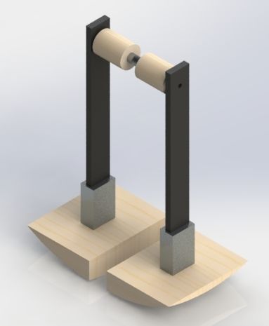
each single support phase of the SPWS. The structural description of each obtained design
is shown in Figure 9, where the CAD rendering of both designs is presented.
Thus, according to Tables 5 and 6 and Figures 7 and 8, the following findings
are observed:
• Integrated S-C design obtains a better synergy between walking capability and ener-
getic efficiency design objectives than the sequential design method. This is demon-
strated by assuming that a better synergy between criteria is when the trade-off in the
aggregate function J ( p∗ ) is minimum, meaning that waking capability and energetic
efficiency are in equilibrium, the proposal reduces around 63.55% the value of the
aggregate function J ( p∗ ) with respect to the sequential design (based on the column
J ( p∗ ) of Table 8). The overall behavior of both designs is shown in Figure 8. Both
designs can develop a gait cycle in the two walking stages, i.e., the walking capability
J1 ( p∗ ) is suitable in both designs. Nevertheless, the proposal reduces 95.41% of the
control activation and its magnitude with respect to the sequential design based on
the values reported in the column J2 ( p∗ ) of Table 8.
• In both design approaches, the proposed semi-passive control strategy can produce
a periodic movement of the SPBR into the SPWS. This achieves the same dynamic
coupling between the frontal plane movement and the gait periods in both the PWS
and SPWS of the sagittal plane (the dynamic coupling is reached in the oscillation
p sp
periods T f ro = Tsag = Tsag = 1.2s, as indicates in Table 7). Thus, the walking capability
for integrated and sequential design is assured.
• The semi-passive control signal is activated around 5% of the SPWS time in the
integrated design (see Table 6 and Figure 8c). Meanwhile, in the sequential design, the
semi-passive control strategy is activated around 89% of the SPWS time (see Figure 8d).
The features of the achieved semi-passive control signal in the integrated design are
attributed to the high amplitude of the potential and kinetic energies oscillation (see
Figure 10). This contributes to keeping the dynamic response of the SPBR into the
corresponding limit cycle for a long time without the control influence. Hence, this
results in the reduction of the control system activation.
• Based on the structure of the SPBR, the center of mass of integrated and sequential
design is located almost at the same height with respect to the leveled ground (see
y y
columns CM f ro and CMsag of Table 7). Nevertheless, the value of mass related to the
integrated design is higher in comparison with the sequential one. In addition, it
is observed that integrated S-C design approach exploit the structural properties of
the SPBR to promote higher angular displacements along the PWS and SPWS. This
fact is shown in Table 9, where the ratio between the maximum angular displace-
ments and the permitted rolling angles in frontal and sagittal plane of the SPBR are
max θ f (t) ≈ 0.81β f ro and max (|θst (t)|, |θsw (t)|) ≈ 0.98δsag , respectively. Mean-
while, for the sequential design these relationships are max θ f (t) ≈ 0.33β f ro and
max (|θst (t)|, |θsw (t)|) ≈ 0.88δsag , respectively. Furthermore, the amplitude of the
movement in frontal plane of the S-C design is associated with the value of R∗f and
θ ∗f i , where in both cases, integrated design approach provides higher values for these
design variables. With respect to the sagittal plane, although the best design of each
approach converged towards the same value of inclination angle γ∗ in the PWS, the
structure and control parameters of the integrated one induced that the angular dis-
placement and velocity are higher in both walking scenarios in comparison with theYou can also read