Introducing the NewHorizon simulation: Galaxy properties with resolved internal dynamics across cosmic time - arXiv
←
→
Page content transcription
If your browser does not render page correctly, please read the page content below
Astronomy & Astrophysics manuscript no. article                                                                                         ©ESO 2021
                                               June 29, 2021

                                                   Introducing the NewHorizon simulation: Galaxy properties with
                                                           resolved internal dynamics across cosmic time
                                                   Yohan Dubois1 , Ricarda Beckmann1 , Frédéric Bournaud2, 3 , Hoseung Choi4 , Julien Devriendt5 , Ryan Jackson6 ,
                                                    Sugata Kaviraj6 , Taysun Kimm4 , Katarina Kraljic7, 8 , Clotilde Laigle1 , Garreth Martin9, 10 , Min-Jung Park4 ,
                                                             Sébastien Peirani11, 1 , Christophe Pichon1, 12, 13 , Marta Volonteri1 , and Sukyoung K. Yi4

                                                      1
                                                          Institut d’Astrophysique de Paris, UMR 7095, CNRS, UPMC Univ. Paris VI, 98 bis boulevard Arago, 75014 Paris, France
                                                          e-mail: dubois@iap.fr
                                                      2
                                                          AIM, CEA, CNRS, Université Paris-Saclay, Université Paris Diderot, Sorbonne Paris Cité, 91191 Gif-sur-Yvette, France
                                                      3
arXiv:2009.10578v4 [astro-ph.GA] 28 Jun 2021

                                                          IRFU, CEA, Université Paris-Saclay, 91191 Gif-sur-Yvette, France
                                                      4
                                                          Department of Astronomy and Yonsei University Observatory, Yonsei University, Seoul 03722, Republic of Korea
                                                          e-mail: yi@yonsei.ac.kr
                                                      5
                                                          Department of Physics, University of Oxford, Keble Road, Oxford OX1 3RH, United Kingdom
                                                      6
                                                          Centre for Astrophysics Research, University of Hertfordshire, College Lane, Hatfield, Herts AL10 9AB, United Kingdom
                                                      7
                                                          Aix Marseille Université, CNRS, CNES, UMR 7326, Laboratoire d’Astrophysique de Marseille, Marseille, France
                                                      8
                                                          Institute for Astronomy, University of Edinburgh, Royal Observatory, Blackford Hill, Edinburgh, EH9 3HJ, United Kingdom
                                                      9
                                                          Steward Observatory, University of Arizona, 933 N. Cherry Ave, Tucson, AZ 85719, USA
                                                     10
                                                          Korea Astronomy and Space Science Institute, 776 Daedeokdae-ro, Yuseong-gu, Daejeon 34055, Republic of Korea
                                                     11
                                                          Université Côte d’Azur, Observatoire de la Côte d’Azur, CNRS, Laboratoire Lagrange, Nice, France
                                                     12
                                                          IPHT, DRF-INP, UMR 3680, CEA, Orme des Merisiers Bat 774, 91191 Gif-sur-Yvette, France
                                                     13
                                                          Korea Institute of Advanced Studies (KIAS) 85 Hoegiro, Dongdaemun-gu, Seoul, 02455, Republic of Korea

                                                     Received / Accepted

                                                                                                                   ABSTRACT

                                                     Hydrodynamical cosmological simulations are increasing their level of realism by considering more physical processes and having
                                                     greater resolution or larger statistics. However, usually either the statistical power of such simulations or the resolution reached within
                                                     galaxies are sacrificed. Here, we introduce the NewHorizon project in which we simulate at high resolution a zoom-in region of
                                                     ∼ (16 Mpc)3 that is larger than a standard zoom-in region around a single halo and is embedded in a larger box. A resolution of up
                                                     to 34 pc, which is typical of individual zoom-in, up-to-date resimulated halos, is reached within galaxies; this allows the simulation
                                                     to capture the multi-phase nature of the interstellar medium and the clumpy nature of the star formation process in galaxies. In
                                                     this introductory paper, we present several key fundamental properties of galaxies and their black holes, including the galaxy mass
                                                     function, cosmic star formation rate, galactic metallicities, the Kennicutt-Schmidt relation, the stellar-to-halo mass relation, galaxy
                                                     sizes, stellar kinematics and morphology, gas content within galaxies and its kinematics, and the black hole mass and spin properties
                                                     over time. The various scaling relations are broadly reproduced by NewHorizon with some differences with the standard observables.
                                                     Owing to its exquisite spatial resolution, NewHorizon captures the inefficient process of star formation in galaxies, which evolve
                                                     over time from being more turbulent, gas rich, and star bursting at high redshift. These high-redshift galaxies are also more compact,
                                                     and they are more elliptical and clumpier until the level of internal gas turbulence decays enough to allow for the formation of discs.
                                                     The NewHorizon simulation gives access to a broad range of galaxy formation and evolution physics at low-to-intermediate stellar
                                                     masses, which is a regime that will become accessible in the near future through surveys such as the LSST.
                                                     Key words. Galaxies: general – Galaxies: evolution – Galaxies: stellar content – Galaxies: kinematics and dynamics – Methods:
                                                     numerical

                                               1. Introduction                                                              formation of the stars. Therefore, cosmological simulations are
                                                                                                                            now a key tool in this theoretical understanding by allowing us
                                               The origin of the various physical properties of galaxies, such              to track the anisotropic non-linear cosmic accretion (which spec-
                                               as their mass content, size, kinematics, or morphology, emerges              tacularly results in filamentary gas accretion; e.g. Kereš et al.
                                               from the complex multi-scale and highly non-linear nature of                 2005; Dekel & Birnboim 2006; Ocvirk et al. 2008) in a self-
                                               the problem. It involves a strong connection between the small-              consistent fashion.
                                               scale star formation embedded in large molecular complexes                       Important challenges exist in the field of galaxy formation
                                               and the gas that is accreted from the intergalactic medium and               that need to be addressed, such as the global inefficiency of the
                                               ejected into large-scale galactic outflows. To draw a theoretical            star formation process on galactic scales (e.g. Moster et al. 2013;
                                               understanding of the process of galaxy formation and evolution,              Behroozi et al. 2013), the morphological diversity of galaxies
                                               it is necessary to connect cosmological structure formation—                 across the whole mass range (e.g. Conselice 2006; Martin et al.
                                               which leads to gas accretion into galaxies, that is the fuel of star         2020), and the important evolution of the nature of galaxies over
                                               formation—to the relevant small-scale processes that lead to the             time; galaxies are more gas rich (e.g. Daddi et al. 2010a) and
                                                                                                                                                                        Article number, page 1 of 29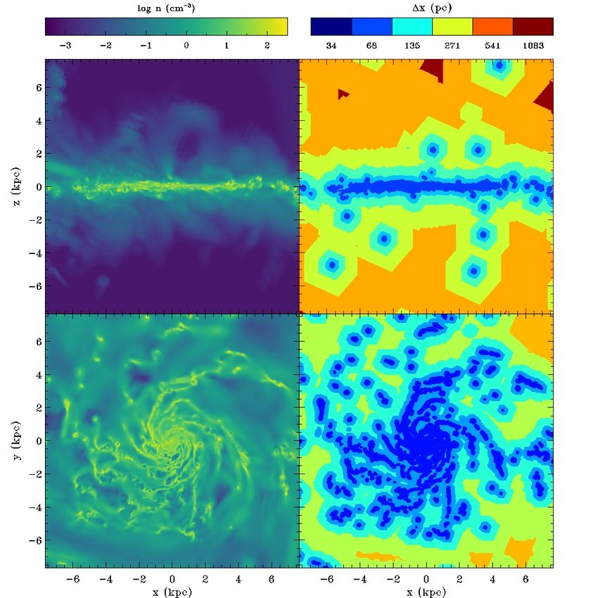
A&A proofs: manuscript no. article

turbulent (e.g. Kassin et al. 2007), clumpy and irregular (e.g.        the IllustrisTNG suite and the Romulus25 simulation (Tremmel
Genzel et al. 2011), and star forming (e.g. Elbaz et al. 2007)         et al. 2017), which offer sub-kiloparsec resolution of 100 and
at early time than they are in the local Universe.                     250 pc, respectively.
    High-redshift galaxies substantially differ in nature from              An important aspect of the evolution of galaxies is that rather
low-redshift galaxies because cosmic accretion is more effi-           than occurring in a homogeneous medium of diffuse interstel-
ciently funnelled to the centre of dark matter (DM) halos ow-          lar gas, star formation proceeds within clustered molecular com-
ing to higher large-scale densities (Dekel et al. 2009), bringing      plexes; these range from pc to 100 pc in size and have properties
gas into galaxies with lower angular momentum, higher surface          that vary from one galaxy to another (e.g. Hughes et al. 2013;
densities, and, hence, more efficient star formation. However,         Sun et al. 2018). This has several important consequences. A
for this high-redshift Universe that is naturally more efficient at    clumpier star formation affects the stellar distribution via a more
feeding intergalactic gas into structures, a significant amount of     efficient migration of stars; it can be locally efficient while glob-
galactic-scale feedback has to regulate the gas budget. On the         ally inefficient, and it can also enhance the effect of stellar feed-
low-mass end, it is generally accepted that stellar feedback as        back by driving more concentrated input of energy. Therefore,
a whole, and more likely feedback from supernovae (SNe), is            the necessity of capturing this minimal small-scale clustering of
able to efficiently drive large-scale galactic winds (e.g. Dekel &     gas in galaxies has constrained numerical simulations to either
Silk 1986; Springel & Hernquist 2003; Dubois & Teyssier 2008;          rely on isolated set-ups (i.e. an isolated disc of gas and stars or
Dalla Vecchia & Schaye 2008), although the exact strength of           isolated spherical collapsing halos; see e.g. Dobbs et al. 2011;
that feedback, and hence, how much gas is driven in and out            Bournaud et al. 2014; Semenov et al. 2018) or on zoomed-in
of galaxies is still largely debated and relies on several impor-      cosmological simulations with a handful of objects (e.g. Cev-
tant physical assumptions (e.g. Hopkins et al. 2012; Agertz et al.     erino et al. 2010; Hopkins et al. 2014, 2018; Dubois et al. 2015;
2013; Kimm et al. 2015; Rosdahl et al. 2017; Dashyan & Dubois          Nuñez-Castiñeyra et al. 2021; Agertz et al. 2021); this is because
2020). On the high-mass end, because of deeper potential wells,        of the strong requisite on spatial resolution, that is typically be-
stellar feedback remains largely inefficient and gas regulation re-    low the 100 pc scale. Since star formation occurs in molecular
lies on the activity of central supermassive black holes (e.g. Silk    clouds that are gravitationally bound or marginally bound with
& Rees 1998; Di Matteo et al. 2005; Croton et al. 2006; Dubois         respect to turbulence, a consistent theory of a gravo-turbulence-
et al. 2010, 2012; Kaviraj et al. 2017; Beckmann et al. 2017).         driven star formation efficiency can be built considering that this
    Low-mass and low surface-brightness regimes are becoming           shapes the probability density function (PDF) of the gas density
important frontiers for the study of galaxy evolution (e.g. Martin     within the cloud (see e.g. Federrath & Klessen 2012, and ref-
et al. 2019) as surveys such as the LSST will allow us to ob-          erences therein). Such a theory can only be used in simulations
serve very faint structures such as tidal streams and, for the first   in which the largest-scale modes of the interstellar medium tur-
time, thousands of dwarfs at cosmological distances (mostly at         bulence are captured (Hopkins et al. 2014; Kimm et al. 2017;
z < 0.5). Complementary high-resolution cosmological simu-             Nuñez-Castiñeyra et al. 2021). Similarly, less ad hoc models for
lations and deep observational datasets will enable us to start        SN feedback can be used to accurately reproduce the distinct
addressing the considerable tension between theory and obser-          physical phases of the blown-out SN bubbles (the so-called Se-
vations in the dwarf regime (e.g. Boylan-Kolchin et al. 2011;          dov and snowplough phases; e.g. Kimm & Cen 2014), depending
Pontzen & Governato 2012; Naab & Ostriker 2017; Silk 2017;             on the exact location of these explosions in the multi-phase ISM.
Kaviraj et al. 2019; Jackson et al. 2021a) as well as in the high-          Our approach in this new numerical hydrodynamical cosmo-
mass regime, where faint tidal features encode information that        logical simulation called NewHorizon, which we introduce in this
can aid in understanding the role of galaxy mergers and interac-       work1 , is to provide a complementary tool between these two
tions in the formation, evolution, and survival of discs (Jackson      standard techniques, that is between the few well-resolved ob-
et al. 2020; Park et al. 2019) and spheroids (Toomre & Toomre          jects versus a large ensemble of poorly resolved galaxies. The
1972; Bournaud et al. 2007; Naab et al. 2009; Kaviraj 2014;            NewHorizon tool is designed to capture the basic features of the
Dubois et al. 2016; Martin et al. 2018a).                              multi-scale, clumpy, ISM with a spatial resolution of the order
    Owing to their modelling of the most relevant aspects of           of 34 pc in a large enough high-resolution, zoomed-in volume
feedback, SNe and supermassive black holes, which occur at             of (16 Mpc)3 . This is larger than a standard zoomed-in halo, has
the two mass ends of galaxy evolution, respectively, and thanks        a standard cosmological mean density, and is embedded in the
to their large statistics, large-scale hydrodynamical cosmologi-       initial lower-resolution (142 Mpc)3 volume of the Horizon-AGN
cal simulations with box sizes of ∼ 50 − 300 Mpc have made             simulation (Dubois et al. 2012); at z = 0.25, the mass density in
a significant step towards a more complete understanding of            that zoom-in region is 1.2 times that of the cosmic background
the various mechanisms (accretion, ejection, and mergers) in-          density. Although still limited in terms of statistics over the en-
volved in the formation and evolution of galaxies; these large-        tire range of galaxy masses (in particular galaxies in clusters are
scale simulations include Horizon-AGN (Dubois et al. 2014a),           not captured), this volume offers sufficient enough statistics – in
Illustris (Vogelsberger et al. 2014), EAGLE (Schaye et al. 2015),      an average density region – to meaningfully study the evolution
IllustrisTNG (Pillepich et al. 2018), SIMBA (Davé et al. 2019),        of galaxy properties at a resolution sufficient to apply more real-
Extreme-Horizon (Chabanier et al. 2020a), and Horizon Run              istic models of star formation and feedback.
5 (Lee et al. 2021). However, as a result of their low spatial reso-        This paper introduces the NewHorizon simulation with its un-
lution in galaxies (typically of the order of 1 kpc), and therefore    derlying physical model and reviews the main fundamental prop-
owing to their intrinsic inability to capture the multi-phase na-      erties of the simulated galaxies, including their mass budget, star
ture of the interstellar medium (ISM), their sub-grid models for        1
                                                                          See Park et al. (2019, 2021); Volonteri et al. (2020); Martin et al.
star formation or the coupling of feedback to the gas has had to       (2021); Jackson et al. (2021a) and Jackson et al. (2021b) for early results
rely on cruder effective approaches than what a higher-resolution      on the origin of discs and spheroids, the thickness of discs, the mergers
simulation might allow. A couple of simulations with an inter-         of black holes, the role of interactions in the evolution of dwarf galaxies,
mediate volume and a better mass and spatial resolution stand          the DM deficient galaxies, and low-surface brightness dwarf galaxies,
out; these are the TNG50 simulation (Pillepich et al. 2019) from       respectively.

Article number, page 2 of 29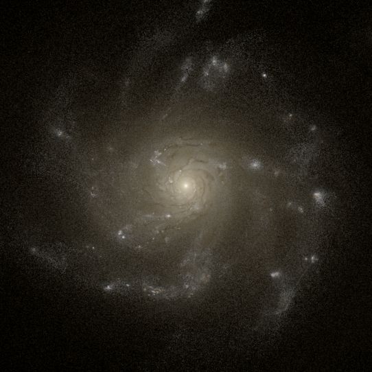
Y. Dubois et al.: The NewHorizon simulation
formation rate (SFR), morphology, kinematics, and the mass and linear interpolation of the cell-centred quantities at cell inter-
spin properties of the hosted black holes in galaxies. faces using a minmod total variation diminishing scheme. Time
The paper is organised as follows. Section 2 presents the nu- steps are sub-cycled on a level-by-level basis, that is each level
merical technique, resolution, and physical models implemented of refinement has a time step that is twice as small as the coarser
in NewHorizon. Section 3 presents the various results of the prop- level of refinement, following a Courant-Friedrichs-Lewy con-
erties of the galaxies in the simulation and their evolution over dition with a Courant number of 0.8. The simulation was run
time. Finally, we conclude in Section 4. down to z = 0.25 using a total amount of 65 single core central
processing unit (CPU) million hours. The simulation contained
typically 0.5-1 billion of leaf cells in total. With 30-100 millions
2. The NewHorizon simulation: Prescription of leaf cells per level of refinement in the zoom-in region from
We describe the NewHorizon simulation employed in this work2 , level 12 to level 22, the region had a total of 3.3 × 10⁸ star parti-
which is a sub-volume extracted from its parent Horizon-AGN cles formed and completed 4.7 × 10⁶ fine time steps (the number
simulation (Dubois et al. 2014a)3 , and the procedure we use to of time steps of the maximum level of refinement), thus, corre-
identify halos and galaxies. A number of physical sub-grid mod- sponding to an average fine time step of size ∆t ' 2.3 kyr), by
els have been substantially modified compared to the physics z = 0.25.
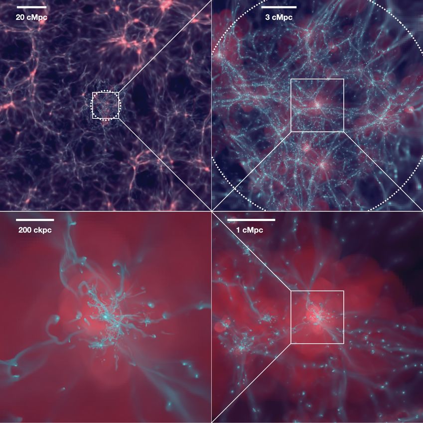
implemented in Horizon-AGN (see e.g. Volonteri et al. 2016; Fig. 1 shows a projection of the high-resolution region. Fig. 2
Kaviraj et al. 2017), in particular regarding the models for star illustrates the typical structure of the gas density achieved in one
formation, feedback from SNe and from active galactic nuclei of the massive galaxies at z = 1 and the corresponding gas res-
(AGN). A comparison with simulated galaxies in Horizon-AGN olution. The diffuse ISM (0.1-1 cm−3 ) is resolved with a ∼100
within the same sub-volume will be the topic of a dedicated pa- pc resolution or such, while the densest clouds reach the max-
per. Nonetheless, we describe the corresponding differences with imum level of refinement corresponding to 34 pc and the im-
Horizon-AGN at the end of each of the subsections of the sub-grid mediate galactic corona is resolved with cells of size 500 pc. In
model. terms of mass and spatial resolution, NewHorizon is comparable
to TNG50 (Pillepich et al. 2019) (4.5 × 10⁵ M DM mass resolu-
tion and a spatial resolution in galaxies of 100 pc) or zoomed-in
2.1. Initial conditions and resolution cosmological simulations (such as for the most massive galaxies
The NewHorizon simulation is a zoom-in simulation from the of the FIRE-2 runs; Hopkins et al. 2018).
142 Mpc size Horizon-AGN simulation (Dubois et al. 2014a).
The Horizon-AGN simulation initial conditions had 10243 DM 2.2. Radiative cooling and heating
particles, a 10243 minimum grid resolution, and a ΛCDM cos-
mology. The total matter density is Ωm = 0.272, dark en- We adopt the equilibrium chemistry model for primordial
ergy density ΩΛ = 0.728, amplitude of the matter power spec- species (H and He) assuming collisional ionisation equilibrium
trum σ8 = 0.81, baryon density Ωb = 0.045, Hubble con- in the presence of a homogeneous UV background. The pri-
stant H0 = 70.4 km s−1 Mpc−1 , and n s = 0.967 is compati- mordial gas is allowed to cool down to ≈ 104 K through col-
ble with the WMAP-7 data (Komatsu et al. 2011). Within this lisional ionisation, excitation, recombination, Bremsstrahlung,
large-scale box, we define an initial spherical patch of 10 Mpc and Compton cooling. Metal-enriched gas can cool further down
radius, which is large enough to sample multiple halos at a to 0.1 K using rates tabulated by Sutherland & Dopita (1993)
40963 effective resolution, that is with a DM mass resolution above ≈ 104 K and those from Dalgarno & McCray (1972) be-
of MDM,hr = 1.2 × 10⁶ M . The high-resolution initial patch is low ≈ 104 K. The heating of the gas from a uniform UV back-
embedded in buffered regions with decreasing mass resolution ground takes place after redshift zreion = 10, following Haardt &
of 107 M , 8 × 10⁷ M , 6 × 10⁸ M for spheres of 10.6 Mpc, Madau (1996). Motivated by the radiation-hydrodynamic simu-
11.7 Mpc, and 13.9 Mpc radius, respectively, and a resolution of lation results that the UV background is self-shielded in optically
5 × 10⁹ M in the rest of the simulated volume. In order to follow thick regions (nH > −3
∼ 0.01 H cm ) (Rosdahl & Blaizot 2012),
the Lagrangian evolution of the initial patch, we fill this initial we assume that UV photo-heating rates are reduced by a factor
sub-volume with a passive colour variable with values of 1 inside exp (−nH /nshield ), where nshield = 0.01 H cm−3 .
and zero outside, and we only allow for refinement when this Compared to Horizon-AGN, the gas can now cool below
passive colour is above a value of 0.01. Within this coloured re- 104 K.
gion, refinement is allowed in a quasi-Lagrangian manner down
to a resolution of ∆x = 34 pc at z = 0: refinement is triggered
if the total mass in a cell becomes greater than eight times the 2.3. Star formation
initial mass resolution. The minimum cell size is kept roughly Star formation occurs in regions with hydrogen gas number
constant by adding an extra level of refinement every time the ex- density above n0 = 10 H cm−3 (the stellar mass resolution is
pansion factor is doubled (i.e. at aexp = 0.1, 0.2, 0.4 and 0.8); the n0 mp ∆x3 = 1.3 × 10⁴ M ) following a Schmidt law: ρ̇? =
minimum cell size is thus between ∆x = 27 and 54 pc. We also ? ρg /tff , where ρ̇? is the SFR mass density, ρg the gas mass den-
added a super-Lagrangian refinement criterion to enforce the re-
sity, tff = 3π/(32Gρg ) the local free-fall time of the gas, G
p
finement of the mesh if a cell has a size shorter than one Jeans’
the gravitational constant, and ? ia varying star formation effi-
length wherever the gas number density is larger than 5 H cm−3 .
ciency (Kimm et al. 2017; Trebitsch et al. 2017, 2020).
The NewHorizon simulation is run with the adaptive mesh
refinement ramses code (Teyssier 2002). Gas is evolved with The current theory of star formation provides a framework
a second-order Godunov scheme and the approximate Harten- for working out the efficiency of the star formation where
Lax-Van Leer-Contact (HLLC Toro 1999) Riemann solver with the gas density PDF is well approximated by a log-normal
PDF (Krumholz & McKee 2005; Padoan & Nordlund 2011;
2
http://new.horizon-simulation.org Hennebelle & Chabrier 2011; Federrath & Klessen 2012). This
3
http://horizon-simulation.org PDF is related to the star-forming cloud properties through the
Article number, page 3 of 29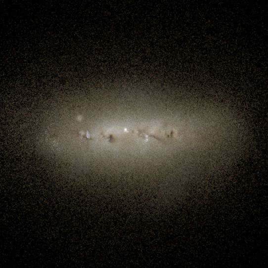
A&A proofs: manuscript no. article
Fig. 1. Sequential zoom (clockwise from top left) over the projected density (silver blue colours) and projected temperature (red) of the
NewHorizon simulation at redshift z = 2. The dashed white circles encompass the initial high-resolution volume. Each panel is a zoomed-in
version of the previous panel (identified by the white square in the previous panel) with the panel sizes of 142, 18, 4.4, and 1.1 comoving Mpc
width, respectively. The two top panels encompass the zoom-in region, with its network of filaments. The two bottom panels illustrate how narrow
filaments break up and mix once they connect to one of the most massive galaxies of that zoom-in region.
cloud turbulent Mach number M = urms /cs , where urms is the where s = ln(ρ/ρ0 ) is the logarithmic density contrast of the PDF
root mean square velocity, cs the sound speed. The virial param- with mean ρ0 and variance σ2s = ln(1+b2 M2 ). In this expression
eter αvir = 2Ekin /Egrav and the efficiency is fully determined by b = 0.4 conveys the fractional amount of solenoidal to compres-
integrating how much mass passes above a given density thresh- sional modes of the turbulence. The critical density contrast scrit
old using the multi-free fall approach of Hennebelle & Chabrier is determined by Padoan & Nordlund (2011) as follows:
(2011) as follows:
σ2s − scrit
!
3
!
? = exp σ2s 1 + erf p
, 0.067
(1) scrit = ln αvir M .
2
(2)
2φt 8 2σ2s θ2
Article number, page 4 of 29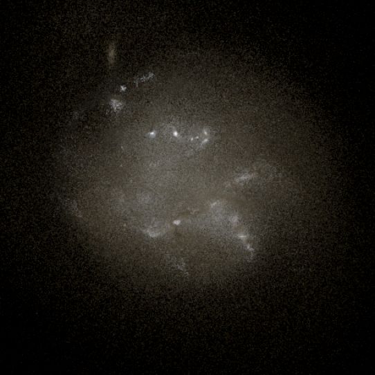
Y. Dubois et al.: The NewHorizon simulation

                                                                             have an efficiency that quickly drops to very low values. Star
                                                                             formation efficiency, in conjunction with stellar feedback, plays
                                                                             a key role in shaping galaxy properties (e.g. Agertz et al. 2011;
                                                                             Nuñez-Castiñeyra et al. 2021), and such potentially higher and
                                                                             more bursty star formation participates in driving stronger out-
                                                                             flows and self-regulation of galaxy properties. We note that our
                                                                             gravo-turbulent model of SF is somewhat reminiscent of those
                                                                             adopted in Hopkins et al. (2014, 2018) or Semenov et al. (2018).
                                                                             In those models, αvir is used as a criterion to trigger star for-
                                                                             mation (gas needs to be sufficiently bound), but star formation
                                                                             proceeds with a constant efficiency in contrast to our model.
                                                                                 Compared to Horizon-AGN, star formation in NewHorizon
                                                                             occurs at above a hundred times larger gas density, and a varying
                                                                             gravo-turbulent-based star formation efficiency is used instead of
                                                                             assuming a constant 2 per cent efficiency.

                                                                             2.4. Feedback from massive stars

                                                                             We include feedback from Type II SNe assuming that each ex-
                                                                             plosion initially releases the kinetic energy of 1051 erg. Because
                                                                             the minimum mass of a star particle is 104 M , each particle is
                                                                             assumed to represent a simple stellar population with a Chabrier
                                                                             initial mass function (IMF) (Chabrier 2005) where the lower (up-
                                                                             per) mass cut-off is taken as Mlow = 0.1 (Mupp = 150) M ,
Fig. 2. Illustration of the structure of the gas density (left panels) and   respectively. We further assume that the minimum mass that ex-
the corresponding spatial resolution (right panels) in a massive galaxy
                                                                             plodes is 6 M in order to include electron-capture SNe (Chiosi
of Ms = 6 × 10¹⁰ M at z = 1 seen edge-on (top panels) or face-on
(bottom panels).                                                             et al. 1992, see also Crain et al. 2015). The corresponding spe-
                                                                             cific frequency of SN explosion is 0.015 M−1 . We increase this
                                                                             number by a factor of 2 (0.03 M−1 ) because multiple clustered
In the NewHorizon simulation, the turbulent Mach number is                   SN explosions can increase the total radial momentum, with re-
given by the local three-dimensional instantaneous velocity dis-             spect to the total momentum predicted by the accumulation of
persion σg (obtained by computing σ2g = sum(∇ ⊗ udx)2 ),                     individual SNe (Thornton et al. 1998), by decreasing the ambi-
and the virial parameter also takes the thermal pressure sup-                ent density into which subsequent SNe explode (Kim et al. 2017;
port αvir,0 = 5(σ2g + c2s )/(πρgG∆x2 ) into account. In this case,           Gentry et al. 2019, Na et al. in prep.). Supernovae are assumed
φ−1                                                                          to explode instantaneously when a star particle becomes older
  t = 0.57 and θ = 0.33 are empirical parameters of the model
determined by the best-fit values between the theory and the nu-             than 5 Myr. The mass loss fraction of a stellar particle from the
merical experiments (Federrath & Klessen 2012). The different                explosions is 31% and has a metal yield (mass ratio of the newly
values of φ−1                                                                formed metals over the total ejecta) of 0.05.
            t and θ we use compared to those given in Feder-
rath & Klessen (2012) arise from the difference between the def-                  We employ the mechanical SN feedback scheme (Kimm
inition of αvir (measured over time, which are the values given              & Cen 2014; Kimm et al. 2015), which ensures the transfer
in Federrath & Klessen 2012) and αvir,0 (the homogeneous cloud               of a correct amount of radial momentum to the surroundings.
initial conditions). As our measurements of the virial parameter             Specifically, the model examines whether the blast wave is in
are meant to correspond to the initial cloud value αvir,0 , that is          the Sedov-Taylor energy-conserving or momentum-conserving
to the virial parameter of a spherical gas cloud with the same               phase (Chevalier 1974; Cioffi et al. 1988; Blondin et al. 1998)
mass, radius, and thermo-turbulent velocity dispersion (Bertoldi             by calculating the mass swept up by SN. If the SN explosion
& McKee 1992; Krumholz & McKee 2005) of the gas cell, we                     is still in the energy-conserving phase, the assumed specific en-
use the best-fit values from Federrath & Klessen (2012) corre-               ergy is injected into the gas since hydrodynamics naturally cap-
sponding to this definition of the virial parameter (Fedderath,              ture the expansion of the SN and imparts the correct amount of
private communication). We ignore the role of the magnetic field             radial momentum. However, if the cooling length in the neigh-
in this model despite the effect it has on the critical density and          bouring regions is under-resolved owing to finite resolution, ra-
variance of the density PDF due to its large pressure with respect           diative cooling takes place rapidly, thereby suppressing the ex-
to the thermal pressure in the cold neutral medium (e.g. Heiles              pansion of the SN bubble. This leads to an under-estimation of
& Troland 2005; Crutcher 2012). In Eq. (1)  = 0.5 is a proto-               the radial momentum, hence weaker feedback. In order to avoid
stellar feedback parameter that controls the actual amount of gas            this artificial cooling, the mechanical feedback model directly
above scrit that is able to form stars (typical estimates of  are           imparts the radial momentum expected during the momentum-
around 0.3 − 0.5; see Matzner & McKee 2000; Alves et al. 2007;               conserving phase if the mass of the neighbouring cell exceeds
André et al. 2010).                                                          some critical value. This is done by first measuring the local ra-
     Such a star formation law shows a significantly different be-           tio of the swept-up gas mass over the ejecta mass and examining
haviour on galactic scales with respect to simulations with con-             whether the ratio is greater than the critical ratio correspond-
stant (usually low) efficiencies since the efficiency can now vary           ing to the energy-to-momentum phase transition. That is to say
                                                                                   −2/17 −4/17 0−0.28
by orders of magnitude. For instance, for gravitationally bound              70 E51      n1    Z      , where E51 is the total energy released in
(αvir < 1) and highly turbulent regions (M > 1), the efficiency              units of 1051 erg, n1 is the hydrogen number density in units of
can go well above 1, while regions that are marginally bound                 cm−3 , and Z 0 = max[Z/Z , 0.01] is the metallicity, normalised to
                                                                                                                     Article number, page 5 of 29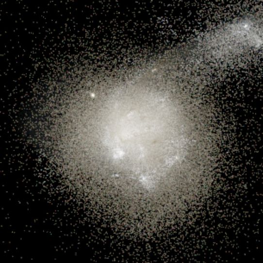
A&A proofs: manuscript no. article

the solar value (Z = 0.02). The final momentum in the snow-               (see Eq: 7) and ṀBondi is the Bondi-Hoyle-Lyttleton rate, that is
plough phase per SN explosion is taken from Thornton et al.
(1998) as                                                                 dMBondi        (GMMBH )2
                                                                                  = 4πρ̄ 2               ,                                (5)
                                                                            dt          (ū + c¯s 2 )3/2
qSN = 3 × 10⁵ km s−1 M E51
                        16/17 −2/17 0−0.14
                             n1    Z       .                       (3)
                                                                          where ū is the average MBH-to-gas relative velocity, c¯s the av-
                                                                          erage gas sound speed, and ρ̄ the average gas density. All aver-
We further assume that the UV radiation from the young OB
                                                                          age quantities are computed within 4∆x of the MBH, using mass
stars over-pressurises the ambient medium near to young stars
                                                                          weighting and a kernel weighting as specified in Dubois et al.
and increases the total momentum per SN to
                                                                          (2012). We do not employ a boost factor in the formulation of
                                                                          the accretion rate, as is commonly done in cosmological simula-
qSN+PH = 5 × 10⁵ km s−1 M E51
                           16/17 −2/17 0−0.14
                                n1    Z       ,                    (4)    tions, because we have sufficient spatial resolution to model part
                                                                          of the multi-phase structure of the ISM of galaxies directly.
following Geen et al. (2015).                                                 The Bondi-Hoyle-Lyttleton accretion rate is capped at the
    It is worth noting that the specific energy used for SN               Eddington luminosity rate for the appropriate r
II explosion in this study is larger than previously assumed.
A Chabrier (2003) IMF with a low- to high-mass cut-off of                 dMEdd 4πGMMBH mp
                                                                               =           ,                                              (6)
Mlow = 0.1 and Mupp = 100 M and an intermediate-to-                        dt      r σT c
massive star transition mass at MIM = 8 M gives eSN =
1.1 × 1049 erg M−1 . However, eSN can be increased up to 3.6 ×            where σT is the Thompson cross-section, m p the proton mass,
1049 erg M−1 if a non-negligible fraction ( fHN = 0.5) of hyper-          and c the speed of light.
                                                                              To avoid spurious motions of MBHs around high-density gas
novae (with EHN ' 1052 erg for stars more massive than 20 M ;
                                                                          regions as a result of finite force resolution effects, we include
e.g. Iwamoto et al. 1998; Nomoto et al. 2006) is taken into ac-
                                                                          an explicit drag force of the gas onto the MBH, following Os-
count. This is necessary to reproduce the abundance of heavy
                                                                          triker (1999). This drag force term includes a boost factor with
elements, such as zinc (Kobayashi et al. 2006), or if a lower
                                                                          the functional form α = (n/n0 )2 when n > n0 , and α = 1 oth-
transition mass MIM = 6 M and a shallower (Salpeter) slope
                                                                          erwise. The use of a sub-grid drag force model is justified by
of −2.1 at the high-mass end (reflecting that early star formation
                                                                          our larger-than-Bondi-radius spatial resolution (Beckmann et al.
should lead to a top-heavier IMF; e.g. Treu et al. 2010; Cappel-
                                                                          2018). We also enforce maximum refinement within a region of
lari et al. 2012; Martín-Navarro et al. 2015) are assumed. Fur-
                                                                          radius 4∆x around the MBH, which improves the accuracy of
thermore, various sources of stellar feedback that would con-
                                                                          MBH motions (Lupi et al. 2015).
tribute to the overall formation of large-scale outflows including
                                                                              The MBHs are allowed to merge when they get closer than
type Ia SNe, stellar winds, shock-accelerated cosmic rays (e.g.
                                                                          4∆x (∼ 150 pc) and when the relative velocity of the pair is
Uhlig et al. 2012; Salem & Bryan 2014; Dashyan & Dubois
                                                                          smaller than the escape velocity of the binary. A detailed analysis
2020), multi-scattering of infrared photons with dust (e.g. Hop-
                                                                          of MBH mergers in NewHorizon is presented in Volonteri et al.
kins et al. 2011; Roškar et al. 2014; Rosdahl & Teyssier 2015), or
                                                                          (2020).
Lyman-α resonant line scattering (Kimm et al. 2018; Smith et al.
2017) are neglected. In addition runaway OB stars (Ceverino &
Klypin 2009; Kimm & Cen 2014; Andersson et al. 2020) or the               2.5.2. Spin evolution of MBH
unresolved porosity of the medium (Iffrig & Hennebelle 2015)
are also ignored. In this regard, the NewHorizon simulation is un-        The evolution of the spin parameter a is followed on-the-fly in
likely to overestimate the effects of stellar feedback, as described      the simulation, taking the effects of gas accretion and MBH-
in Section 3.                                                             MBH mergers into account. The model of MBH spin evolution
    Unlike Horizon-AGN, feedback from stars in NewHorizon                 is introduced in Dubois et al. (2014c), and technical details of
only includes Type II SNe and ignores stellar winds and Type              the model are detailed in that paper. The only change is that we
Ia SNe. In addition, NewHorizon adopts a mechanical scheme                now use a different MBH spin evolution model at low accretion
for SNe instead of a kinetic solution (Dubois & Teyssier 2008).           rates: χ = ṀMBH / ṀEdd < χtrans , where χtrans = 0.01. At high
The assumed IMF is also changed from the Salpeter IMF to a                accretion rates (χ ≥ χtrans ), a thin accretion disc solution is as-
Chabrier type, and thus the mass loss, energy, and yield are all          sumed (Shakura & Sunyaev 1973), as in Dubois et al. (2014c).
increased.                                                                The angular momentum direction of the accreted gas is used to
                                                                          decide whether the accreted gas feeds an aligned or misaligned
                                                                          Lense-Thirring disc precessing with the spin of the MBH (King
2.5. MBHs and AGN                                                         et al. 2005), thereby spinning the MBH up or down for co-
                                                                          rotating and counter-rotating systems, respectively (see top panel
We now briefly describe the models corresponding to massive               of Fig. 3). At low accretion rates (χ < 0.01), we assume that jets
black hole (MBH) formation and their AGN feedback.                        are powered by energy extraction from MBH rotation (Bland-
                                                                          ford & Znajek 1977) and that the MBH spin magnitude can only
2.5.1. Formation, growth, and dynamics of MBH                             decrease. The change in the spin magnitude da/dM follows the
                                                                          results from McKinney et al. (2012), where we fitted a fourth-
In NewHorizon, MBHs are assumed to form in cells that have                order polynomial to their sampled values; from their table 7, sH
gas and stellar densities above the threshold for star formation,         for AaN100 runs, where a is the value of the MBH spin. The
a stellar velocity dispersion larger than 20 km s−1 , and that are        functional form of the spin evolution as a function of MBH spin
located at a distance of at least 50 comoving kpc from any pre-           at low accretion rates is represented in the top panel of Fig. 4,
existing MBH.                                                             where the dimensionless spin-up parameter s ≡ d(a/M)/dt is
    Once formed, the mass of MBHs grows at a rate ṀMBH =                 shown, where if s and a have opposite signs the black hole spins
(1 − r ) ṀBondi , where r is the spin-dependent radiative efficiency   down.
Article number, page 6 of 29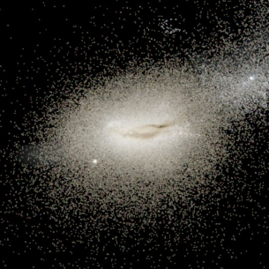
Y. Dubois et al.: The NewHorizon simulation

                               6
                                                                                                                       5

                                                                                                   MCAD Spin up rate
                               5
                Spin up rate

                               4
                                                                                                                       0
                               3

                               2

                               1                                                                                       -5

                               0
                                                                                                                150
                               40                                                                                             jet
                                                                                                                              wind

                                                                                   MCAD eff. (per cent)
     Rad. eff. (per cent)

                                                                                                                              total
                               30
                                                                                                                100

                               20
                                                                                                                       50
                               10

                               0                                                                                       0
                               -1.0   -0.5     0.0     0.5          1.0                                                -1.0           -0.5     0.0            0.5          1.0
                                             BH spin                                                                                         BH spin

Fig. 3. Spin-up rate (top panel) and radiative efficiency rad / fatt (bottom   Fig. 4. Spin-up rate (top panel), jet (red plus signs), wind (blue dia-
panel) as a function of the MBH spin for the thin disc solution (Shakura        monds), and total (black) efficiencies (bottom panel) as a function of
& Sunyaev 1973) applied to the quasar mode. At negative values of the           the MBH spin for the MCAD solution applied to the radio mode. The
MBH spin, the gas accreted from the thin accretion disc decreases the           symbols represent the results from the simulations of McKinney et al.
MBH spin, while for a positive MBH spin, the gas increases. For the             (2012) and the solid lines indicate the interpolated functions used in the
thin disc solution, the radiative efficiency is an increasing function of       NewHorizon simulation. As opposed to the thin disc solution (Fig. 3),
the MBH spin with a sharp increase (by 4) between a MBH spin of 0.7             gas accreted from the thick accretion disc always decreases the MBH
and 0.998.                                                                      spin. The MCAD feedback efficiency is an increasing function of the ab-
                                                                                solute value of the BH spin with a minimum efficiency for non-rotating
                                                                                MBHs.
     In addition, MBH spins change in magnitude and direction
during MBH-MBH coalescences, with the spin of the remnant
depending on the spins of the two merging MBHs and the or-                      releases only thermal energy back into the gas (a.k.a. quasar
bital angular momentum of the binary, following analytical ex-                  mode, Teyssier et al. 2011). The AGN releases a power that is
pressions from Rezzolla et al. (2008).                                          a fraction of the rest-mass accreted luminosity onto the MBH,
     The evolution of the spin parameter is a key component of                  LAGN,R,Q = ηR,Q ṀMBH c2 , where the subscripts R and Q stand for
the AGN feedback model because it controls the radiative ef-                    the radio jet mode and quasar heating mode, respectively.
ficiency of the accretion disc and the jet efficiency. Therefore,                   For the jet mode of AGN feedback, the efficiency ηR is not a
the Eddington mass accretion rate, used to cap the total accre-                 free parameter. This value scales with the MBH spin, following
tion rate, and the AGN feedback efficiency in the jet and thermal               the results from magnetically chocked accretion discs (MCAD)
modes vary with spin values. The spin-dependent radiative effi-                 of McKinney et al. (2012), where we fitted a fourth-order poly-
ciency (see bottom panel of Fig. 3) is defined as                               nomial to the sampled values of jet plus wind efficiencies of this
                                                                              work (from their table 5, η j plus ηw,0 for runs AaN100). This fit
r = fatt (1 − eisco ) = fatt 1 − 1 − 2/(3risco ) ,
                                 p
                                                              (7)               is shown in the bottom panel of Fig. 4. When active in our simu-
                                                                                lation, the bipolar AGN jet deposits mass, momentum, and total
where eisco is the energy per unit rest mass energy of the inner-               energy within a cylinder of size ∆x in radius and semi-height,
most stable circular orbit (ISCO), risco = Risco /Rg is the radius of           centred on the MBH, whose axis is (anti)aligned with the MBH
the ISCO in reduced units, and Rg is half the Schwarzschild ra-                 spin axis (zero opening angle). Jets are launched with a speed of
dius of the MBH. The parameter Risco depends on spin a. For the                 104 km s−1 , whose exact value has little impact on MBH growth
radio mode, the radiative efficiency used in the effective growth               or galaxy mass content (Dubois et al. 2012).
of the MBH is attenuated by a factor fatt = min(χ/χtrans , 1) fol-                  The quasar mode of AGN feedback deposits internal energy
lowing Benson & Babul (2009). The MBH seeds are initialised                     into its surrounding within a sphere of radius ∆x, within which
with a zero spin value and a maximum value of the BH spin at                    the specific energy is uniformly deposited (uniform temperature
amax = 0.998 (due to the emitted photons by the accretion disc                  increase). Because only a fraction of the AGN-driven wind is
captured by the MBH; Thorne 1974) is imposed.                                   expected to thermalise and only some of the multiwavelength
                                                                                radiation emitted from the accretion disc couples to the gas on
                                                                                ISM scales (Bieri et al. 2016), we scale the feedback efficiency
2.5.3. Radio and quasar modes of AGN feedback
                                                                                in quasar mode by a coupling factor of ηc = 0.15, which is cal-
Active galactic nuclei feedback is modelled in two different ways               ibrated on the local MMBH -Ms in lower resolution (∼kpc) simu-
depending on the Eddington rate (Dubois et al. 2012): below                     lations (Dubois et al. 2012). The effective feedback efficiency in
χ < χtrans the MBH powers jets (a.k.a. radio mode) contin-                      quasar mode is therefore ηQ = r ηc .
uously releasing mass, momentum, and total energy into the                          Compared to Horizon-AGN, NewHorizon now includes MBH
gas (Dubois et al. 2010), while above χ ≥ χtrans the MBH                        spin evolution, which affects several compartments of MBH
                                                                                                                                                       Article number, page 7 of 29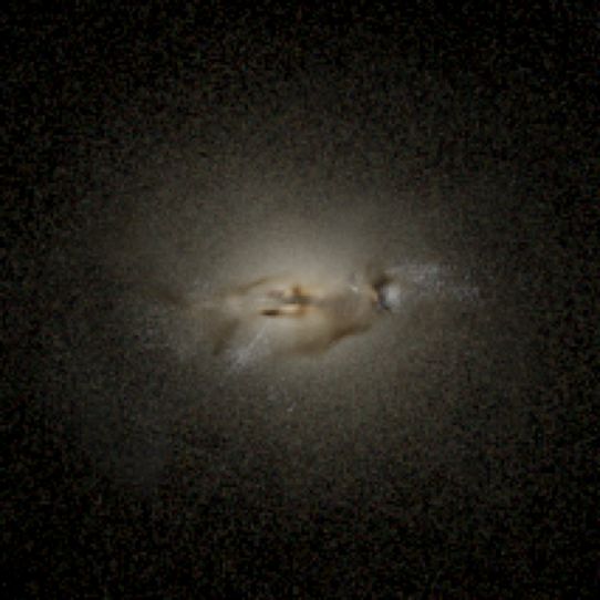
A&A proofs: manuscript no. article

mass growth and feedback. The MBH accretion is changed ow-             Table 1. Number of galaxies for different stellar mass thresholds. Purity
ing to the spin-dependent radiative efficiency, thereby changing       is indicated as a threshold in the percentage of high resolution DM par-
                                                                       ticles of the host halo (in number of DM particles). This work employs
the maximum Eddington accretion rate. The AGN feedback is              the 100% purity sample by default except when indicated.
also changed by the spin-dependent radiative efficiency in the
quasar mode. For the radio mode, the jet closely follows the
spin-dependent mechanical efficiency of the MCAD model in-               Purity    Redshift      Ms >        Ms >        Ms >        Ms >
stead of a constant efficiency of 1, and the jet direction is now         (%)                   107 M       108 M       109 M       1010 M
along the BH spin axis instead of along the accreted gas angular          100           4        688         148          12           0
momentum.                                                                 99.9          4        697         152          12           0
                                                                           99           4        722         157          12           0
                                                                          100           2        626         245          53           5
                                                                          99.9          2        884         342          75           5
2.6. Identification of halos and galaxies                                  99           2        931         364          84           7
                                                                          100           1        403         191          70          12
Halos are identified with the AdaptaHOP halo finder (Aubert               99.9          1        649         310         112          18
et al. 2004). The density field used in AdaptaHOP is smoothed              99           1        732         362         132          23
over 20 particles. The minimum number of particles in a halo is           100         0.25       276         145          58          16
100 DM particles. We only consider halos with an average over-            99.9        0.25       443         238          99          28
density with respect to the critical density ρc , which is larger          99         0.25       531         285         121          32
than δt = 80 and which overcomes   √ the Poissonian noise filter-
ing density threshold at (1 + 5/ N)δt ρc (where N is the number
of particles in the (sub)structure; see Aubert et al. 2004, for de-
tails). For a substructure, it is only kept if the maximum density     3. Cosmic evolution of baryons
is 2.5 times its mean density. The centre of the halo is recursively
determined by seeking the centre of mass in a shrinking sphere,        In this section we present several standard properties of the sim-
while decreasing its radius by 10 per cent recurrently down to         ulated galaxies including their stellar and gas mass content, SFR,
a minimum radius of 0.5 kpc (Power et al. 2003). The maxi-             morphological and structural properties, and kinematics. We also
mum DM density in that radius is defined as the centre of the          present their hosted MBHs and compare these to observational
halo. The shrinking sphere approach is used since strong feed-         relations down to the lowest redshift reached out by the simula-
back processes can significantly flatten the central DM density        tion (z = 0.25).
and smaller, but denser, substructures can be misidentified as be-
ing the centre of the main halo.
                                                                       3.1. Synthetic galaxy morphology
    We run the same identification technique, using either Adap-
taHOP or HOP, on stars to identify the galaxies in the simulation,     In order to qualitatively illustrate the variety of galaxy properties
except that we only consider galaxies with more than 50 star           simulated in NewHorizon, we show in Fig. 5 a couple of galax-
particles and a value of δt twice as large. The AdaptaHOP tool         ies at z = 4, z = 2 and z = 0.25 with their gas density and
separates substructures that include in situ star-forming clumps       stellar emission. The 15 panels on the left show the images of
as well as satellites already connected to a galaxy, while HOP         a massive galaxy (stellar mass Ms = 3.0 × 10⁸ M at z = 4,
keeps all substructures connected to the main structure (i.e. it       8.2 × 10⁹ M at z = 2 and 5.5 × 10¹⁰ M at z = 0.25) and the 15
does not detect substructures). Appendix B shows examples of           panels on the right represent a less massive galaxy (9.7 × 10⁷ M
how using HOP or AdaptaHOP affect the segmentation of galax-           at z = 4, 1.4 × 10⁹ M at z = 2 and 4.0 × 10⁹ M at z = 0.25).
ies. Both tools can be employed depending on context, as indi-         While the first, second, and fourth rows show their gas density
cated in the corresponding text. For the centring of the galaxies      maps, the third and fifth rows show the mock images; the sec-
at the low-mass end, particular attention has to be taken, since       ond and third rows are shown with a face-on view (with respect
these galaxies tend to be extremely turbulent structures where         to the stellar angular momentum of the galaxy) and the fourth
bulges cannot be easily identified.                                    and fifth rows an edge-on view. The mock images are in SDSS
                                                                       g-r-i bands and are generated via the SKIRT9 code (Camps &
    Since the NewHorizon simulation is a zoom simulation em-           Baes 2020), which computes radiative transfer effects based on
bedded in a larger cosmological volume filled with lower DM            the properties and positions of stars and the dusty gas assuming
resolution particles, we also need to remove halos of the zoom         a dust fraction fdust = 0.4 following Saftly et al. (2015). The
regions polluted with low-resolution DM particles. To that end,        high resolution of NewHorizon (34 pc) reveals the detailed struc-
we only consider halos as well as the embedded galaxies and            ture of the cosmologically simulated galaxies, and it is clearly
MBHs encompassed in their virial radius, which are found de-           evident that star formation (highlighted by the young blue re-
void of low-resolution DM particles up to some threshold (see          gion in the stellar maps) proceeds in clustered regions of dense
Appendix A for the halo mass function for different purity lev-        gas. The massive galaxy settles its disc around z ≈ 2.5 and ap-
els). With 100 % purity, there are, respectively, 626, 245, 53,        pears as a regular disc galaxy with well-defined spiral arms and
and 5 main galaxies (which are not substructures in the sense of       a central bulge if witnessed at z = 0.25. We used the visual in-
AdaptaHOP) at z = 2 with stellar mass above 107 , 108 , 109 , and      spection as well as (V/σ)gas > 3 (Kassin et al. 2012) for disc
1010 M ; 403, 191, 70, and 12 at z = 1; and 276, 145, 58, and 16       settling criteria; the calculation of the kinematics is detailed in
at z = 0.25. For comparison, considering a contamination lower         Section 3.13. The less massive galaxy, on the other hand, ex-
than 1 per cent in number of DM, the number of galaxies typi-          hibits an extremely irregular morphology at z = 2 with strong
cally doubles at z = 0.25 (see Table 1 for detailed numbers). We       asymmetries in both gas and stars, and prominent off-centred
note that the most massive unpolluted halo obtained at z = 0.25        (blue) star-forming clusters. This low-mass galaxy, which only
has a DM virial mass of 8 × 10¹² M .                                   grows moderately by z = 0.25, develops a galactic-scale disc at
Article number, page 8 of 29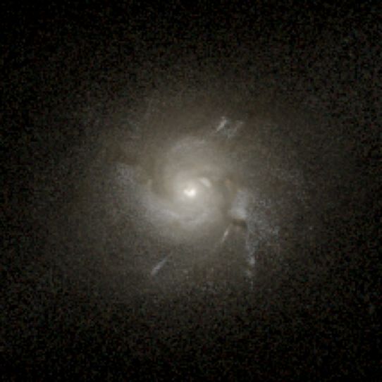
Y. Dubois et al.: The NewHorizon simulation

              10   4        10   3              10   2        10   1

                                     g cm   2

    z= 4.0                 z= 2.0                        z= 0.25                  z= 4.0               z= 2.0              z= 0.25

   log(M): 8.48 10.56 log(M): 9.91 11.34 log(M): 10.74 12.05                     log(M): 7.99 10.42 log(M): 9.14 10.93 log(M): 9.61 11.24

Fig. 5. Projection of the gas density and mock observations. Panels on the left are images of a massive galaxy at different epochs and the panels
on the right are for a less massive galaxy. The first row shows gas density projections a of 1.4 Mpc at different epochs, while the second and fourth
rows are zoomed-in gas density projections with face-on and edge-on views of the galaxy, respectively. Third and fifth rows are SKIRT mock
observations in face-on and edge-on direction. Stellar mass and halo mass of each galaxy at each epoch are given in the second row in log scale.
For a galaxy at a given epoch, the second to fifth panels are on the same scale and the white bar in third row indicates 5 kpc. Gas density maps
share the same colour scheme as given in the colour bar.

z ≈ 1.0 and maintains the marginally stable disc for the rest of               larger than the 20 Mpc box length, it is likely that we do not cap-
the cosmic history.                                                            ture the full variance in the mass function since cosmic variance
                                                                               would be underestimated along the radial axis.

3.2. Galaxy mass function                                                          To infer the stellar masses of the HSC-SSP sample, we
                                                                               use the spectral energy distribution (SED) fitting code LePhare
We compare the z = 0.25 mass function obtained from                            (Arnouts et al. 1999; Ilbert et al. 2006; Arnouts & Ilbert 2011)
NewHorizon with the mass function obtained from an equivalent                  with the Bruzual & Charlot (2003) (BC03 here and after) tem-
volume in the HSC-SSP survey (Aihara et al. 2019). In order to                 plates to estimate galaxy stellar masses from the g, r, i, and z
do this we take 100 random pointings from the HSC-SSP deep                     cModel magnitudes. We then use the luminosity function tool
layer (encompassing the SXDS, COSMOS, ELIAS, and DEEP-                         alf (Ilbert et al. 2005) to construct galaxy stellar mass functions
2 fields), where each pointing has an equivalent volume to the                 for each pointing using the method of Sandage et al. (1979).
NewHorizon box. The central redshift of each volume is varied                  Galaxies are selected in the r band with an apparent magnitude
by up to 0.02 around a central redshift of z = 0.25 for each ran-              cut of 26. We first constrain the knee of the mass function (Ms )
dom pointing. Since the photometric redshift errors are typically              by computing the mass function for each pointing in a larger red-
                                                                                                                       Article number, page 9 of 29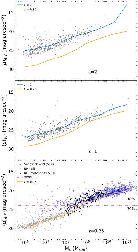
A&A proofs: manuscript no. article

shift slice (0.1 < z < 0.4) before re-fitting the mass function with                              z = 0.25
                                                                                                                          NH (raw)
                                                                                                                          NH (uncontaminated)            z=1
Ms fixed for the smaller volume. For the simulated sample we                                                              NH (STY w/selection effects)
                                                                                        10   1                            HSC-SSP DR2 (STY)
follow a similar procedure, first obtaining dust-attenuated g, r,

                                                                       (cMpc 3 dex 1)
i, and z magnitudes for galaxies identified with HOP using Sun-
                                                                                        10   2
set (see Martin et al. 2021, section 2.2.1). To approximate the
selection effects present in real data, we select galaxies by their
                                                                                        10   3    Fontana+04 (K20, 0.2 < z < 0.7)
                                                                                                  Pozzetti+07 (VVDS, 0.05 < z < 0.4)
effective surface brightness, where the probability of selecting a                                Bielby+12 (WIRDS, 0.2 < z < 0.4)
                                                                                                  Baldry+12 (GAMA), z < 0.06
galaxy is proportional to the surface brightness completeness of                                  Bernardi+13 (SDSS)                                     Fontana+04 (K20, 0.7 < z < 1)
                                                                                        10   4    Ilbert+13 (UltraVISTA, 0.2 < z < 0.5)
                                                                                                  Tomczak+14 (ZFOURGE, 0.2 < z < 0.5)
                                                                                                                                                         Pozzetti+07 (VVDS, 0.9 < z < 1.2)
                                                                                                                                                         Bielby+12 (WIRDS, 1 < z < 1.2)
the HSC survey; this value is estimated by assuming that the true                                 D'Souza+15 (SDSS), z < 0.5                             Ilbert+13 (UltraVISTA, 0.8 < z < 1.1)
                                                                                                  Davidzon+17 (COSMOS, 0.2 < z < 0.5)                    Tomczak+14 (ZFOURGE, 1 < z < 1.5)
number of objects continues to rise exponentially as a function                                   Sedgwick+19 (Stripe 82, CCSNe, z < 0.25)               Davidzon+17 (COSMOS, 0.8 < z < 1.1)
of effective surface brightness after the turnover in the number                        10   5
                                                                                                  z=2                                                    z=4
of galaxies observed by HSC. We again use LePhare and alf
to construct the galaxy stellar mass function using the same 26                         10   1

                                                                       (cMpc 3 dex 1)
mag cut in the r band. Because of the more limited volume of
NewHorizon, the number of galaxies that are considerably more                           10   2

massive than the knee of the mass function is too small to effec-
tively constrain this value, thereby leading to unrealistic fits. We                    10   3

therefore fix Ms at a value of 1010.8 M , which is calculated from                                                                                       Fontana+04 (K20, 1.5 < z < 2)

the full volume of the Horizon-AGN simulation. While varying                            10   4
                                                                                                  Pozzetti+07 (VVDS, 1.6 < z < 2.5)
                                                                                                                                                         Gonzalez+11 (ERS, z 4)
                                                                                                                                                         Ilbert+13 (UltraVISTA, 3 < z < 4)
                                                                                                  Ilbert+13 (UltraVISTA, 2 < z < 2.5)                    Grazian+15 (UDF + GOODS-S, 3.5 < z < 4.5)
                                                                                                  Tomczak+14 (ZFOURGE, 2 < z < 2.5)                      Song+16 (UDF + GOODS-N/S, z~4)
Ms also necessarily affects the slope at the low-mass end, this                                   Davidzon+17 (COSMOS, 2 < z < 2.5)                      Davidzon+17 (COSMOS, 3.5 < z < 4.5)
is not significant enough to qualitatively alter our comparison to                      10 10
                                                                                           5
                                                                                              7        108            109 1010                1011 107        108            109 1010                1011
the observed mass functions within a reasonable range of values                                                       Ms/Msun                                                Ms/Msun
(e.g. 1010.6 M to 1011 M ).                                             Fig. 6. Galaxy stellar mass function at z = 0.25 in NewHorizon and
    The galaxy mass function, which is a volume-integrated              the HSC-SSP survey. The light blue squares and dark blue circles with
quantity poses a conceptual challenge to a zoom-in simulation.          error bars indicate the NewHorizon stellar mass function for all galaxies
                                                                        (offset by 0.15 dex) and only uncontaminated galaxies (with a volume
Indeed, galaxies within halos polluted with low-resolution DM           correction applied). The black line indicates the median galaxy stellar
particles continue to form stars, and it is questionable whether or     mass function from 100 random pointings from a volume of the HSC-
not their contribution to the overall cosmic star formation should      SSP deep layer with the same volume as NewHorizon and the black
be taken into account. In addition, we have to determine the ac-        error bar indicates the 90 percentile scatter in the mass function at the
tual corresponding volume of the zoom-in region, which can ex-          low-mass end. A comparison is made with additional mass functions
pand or contract over time. For the volume entering the calcula-        from literature (Sedgwick et al. 2019; Davidzon et al. 2017; Tomczak
tion of the galaxy mass function (and in other volume-integrated        et al. 2016; Song et al. 2016; Grazian et al. 2015; D’Souza et al. 2015;
quantities measured in this work), we take the entire initial vol-      Fontana et al. 2014; Bernardi et al. 2013; Ilbert et al. 2013; Baldry et al.
ume of the zoom-in region of the simulation, hence, (16 Mpc)3 .         2012; Bielby et al. 2012; González et al. 2011; Pozzetti et al. 2007),
We could alternatively use the sum of each individual leaf cell         which are shown as thin coloured lines. The thick purple dotted line
                                                                        indicates the NewHorizon mass function constructed using the Sandage
that passes a given threshold value of the passive scalar colour        et al. (1979) method (STY) and including selection effects.
value (see Section 2.1). The corresponding initial volume can be
reduced by 20-40 per cent for a threshold value of resp. 0.1- 0.9,
depending on redshift. We decided to simplify the problem by                Once selection effects are included, the NewHorizon mass
taking the initial zoom-in volume, but we note that the presented       function lies within the upper range of the observational mass
volume-integrated quantities are only a lower limit and can be a        functions shown. The discrepancy between the raw mass func-
few tens of per cent higher.                                            tion likely emerges from incompleteness in the observed data
    Figure 6 shows the galaxy stellar mass function from                at low surface brightness, meaning the observed mass function
NewHorizon, HSC-SSP, and from the literature (Sedgwick et al.           may be underestimated towards lower mass. The effect of selec-
2019; Davidzon et al. 2017; Tomczak et al. 2016; Song et al.            tion effects and environment on the galaxy stellar mass function
2016; Grazian et al. 2015; D’Souza et al. 2015; Fontana et al.          will be explored in more detail in Noakes-Kettel et al. (in prep.).
2014; Bernardi et al. 2013; Ilbert et al. 2013; Baldry et al. 2012;         The 90 per cent variance in the low-mass end of the HSC
Bielby et al. 2012; González et al. 2011; Pozzetti et al. 2007).        mass function is indicated by a black error bar. Over such a lim-
We note that Sedgwick et al. (2019) includes only star-forming          ited volume, the normalisation of the galaxy stellar mass func-
galaxies. The light blue squares with error bars represent the          tion varies significantly. We note that our estimate of the vari-
NewHorizon stellar mass function with Poisson errors for all            ance may be an underestimate as redshift uncertainties are sig-
galaxies. The purple circles show the same, but include only            nificantly larger than the selected volume. Additionally the lo-
galaxies whose halos are not contaminated by low-resolution             cation of the four HSC-SSP deep fields were chosen to enable
particles from outside of the highest resolution zoom region –          certain science goals and not necessarily to sample representa-
a simple correction is made to account for the smaller effec-           tive volumes of the Universe as a whole.
tive volume by dividing the mass function by the fraction of
uncontaminated galaxies. Additionally, the mass function (with          3.3. Surface brightness-to-galaxy mass relation
selection effects) for NewHorizon that is constructed using the
Sandage et al. (1979) method (STY) is shown as a thick purple           While many comparisons between theory and observation treat
dotted line. The black line indicates the median galaxy stellar         galaxies as one-dimensional points, the two-dimensional distri-
mass function from the 100 random pointings from the HSC-               bution of baryons (e.g. as summarised by the effective surface
SSP deep layer. Various other mass functions from the literature        brightness and effective radius) are important points of compar-
are also indicated as thin coloured lines in each panel.                ison. Since high-resolution cosmological simulations now offer
Article number, page 10 of 29
Y. Dubois et al.: The NewHorizon simulation
shift for each galaxy from the conditional probability distribu-
tion Pz (M s ) (i.e. the redshift probability distribution at a given
stellar mass as found in Sedgwick et al. 2019) so that they are
redshifted and their flux and size are calculated according to a
redshift whose probability is related to the stellar mass of the
object. The SEDs are then convolved with the response curve
for the SDSS r-band filter. We then weight by the particle mass
to obtain the luminosity contribution of each star particle, and
obtain the apparent r-band magnitude by converting the flux to a
magnitude and adding the distance modulus and zero point.
The second moment ellipse is obtained by firstly construct-
ing the covariance matrix of the intensity-weighted second order
central moments (sometimes called the moment of inertia) for
all the star particles, that is
" 2 #
I x I xy
cov[I(x, y)] = , (8)
I xy Iy2
where I is the flux, and x and y are the projected positions from
the barycentre in √ arcseconds of each star particle
√ in the galaxy.
The major (α = λ1 /ΣI) and minor (β = λ2 /ΣI) axes of the
ellipse are obtained from the covariance matrix, where λ1 and λ2
are its eigenvalues and ΣI is the total flux. The scaling factor, R,
scales the ellipse so that it contains half the total flux of the ob-
ject. Finally, the mean surface brightness within the effective ra-
dius can be calculated from hµie,r = m−2.5log10 (2)+2.5log10 (A),
where A = R2 αβπ and m is the r-band apparent magnitude of the
object. We repeat this process in multiple orientations (xy, xz
and yz), taking the mean surface brightness for each object. The
method presented in this work is equivalent to the method em-
ployed in SExtractor (Bertin & Arnouts 1996) to derive basic
shape parameters, which Sedgwick et al. (2019) use to derive
their measurements.
In Fig. 7, we show the evolution of the surface brightness
hµie,r versus stellar mass plane in NewHorizon. In the bottom
Fig. 7. Surface brightness vs. stellar mass in the NewHorizon simula- panel we compare the predicted surface brightnesses to a recent
tion for 3 redshifts. The grey points indicate the entire galaxy population work that uses the IAC Stripe 82 Legacy Survey project (Sedg-
of NewHorizon in all 3 panels with the median lines for the redshift in wick et al. 2019; Sedgwick et al. 2019). This study is one of few
question and z=0.25 shown in blue and orange, respectively. In the bot- that probes the surface brightnesses of galaxies down into the
tom panel the open blue points indicate galaxies from Sedgwick et al. dwarf regime, which is only possible at low redshift using past
(2019) and black points are NewHorizon galaxies. The predicted sur- and current surveys, which are typically very shallow. To probe
face brightness vs. stellar mass plane in NewHorizon corresponds well galaxy surface brightness down to faint galaxies Sedgwick et al.
to that where the Sedgwick et al. galaxies are complete. The red dotted
introduce a novel technique with core-collapse SNe (CCSNe).
lines in the bottom panel indicate the 70% and 10% completeness limits
from the SDSS (see e.g. Table 1 in Blanton et al. 2005). The overwhelm- Using custom settings in SExtractor (Bertin & Arnouts 1996)
ing majority of galaxies in the Universe lie below the surface brightness they extract the host galaxies of these CCSNe, including those
thresholds of surveys such as the SDSS; only those galaxies that depart that are not detected in the IAC Stripe 82 Legacy survey. The
strongly from the typical surface brightness vs. stellar mass relation are resultant sample is free of incompleteness in surface brightness
likely to be detectable in these datasets. in the stellar mass range Ms > 108 M ; a host is identified for all
707 CCSNe candidates at z < 0.2. Given the high completeness
of the sample at low surface brightness and the relative ease with
predictions of the distribution of baryons, it is worth comparing which we can model the selection function and apply it to our
these predictions to observational data of galaxy surface bright- simulated data, this dataset is an ideal choice to compare to the
nesses. NewHorizon data. More details on how the matching between the
Here, we obtain the dust attenuated surface brightness for two datasets has been completed are available in Jackson et al.
each NewHorizon galaxy using the intensity-weighted second or- 2021a.
der central moment of the stellar particle distribution (e.g. Bern- Figure 7 shows that the surface brightness versus stellar mass
stein & Jarvis 2002) and we compare these values with Sedgwick plane in NewHorizon corresponds well to Sedgwick et al. (2019),
et al. (2019). where the observational data is complete; we note that the sim-
For each star particle, we first obtain the full SED from a ulation is not calibrated to reproduce galaxy surface brightness.
grid of dust attenuated BC03 simple stellar population models The flattening seen in the observations is due to high levels of in-
corresponding to the age and metallicity of the star particle. We completeness at Ms < 108 M . The prediction for the evolution
redshift each BC03 template to match the overall redshift distri- of this plane to higher redshifts shows that NewHorizon galaxies
bution of the observed sample to account for surface-brightness have increasing brightness at higher redshift for a fixed stellar
dimming. Since low-mass galaxies in this sample are biased to- mass (i.e. galaxies are more concentrated, see Section 3.7) can
wards lower redshift, we also account for this by drawing a red- be tested using data from future instruments such as the LSST.
Article number, page 11 of 29You can also read