Exoplanet Atmospheres - Sara Seager
←
→
Page content transcription
If your browser does not render page correctly, please read the page content below
Annual Reviews of Astronomy and Astrophysics
To appear in September 2010

Exoplanet Atmospheres
Sara Seager (MIT) and Drake Deming (NASA/GSFC)

Abstract

At the dawn of the first discovery of exoplanets orbiting sun-like stars in the mid-1990s,
few believed that observations of exoplanet atmospheres would ever be possible. After
the 2002 Hubble Space Telescope detection of a transiting exoplanet atmosphere,
many skeptics discounted it as a one-object, one-method success. Nevertheless, the
field is now firmly established, with over two dozen exoplanet atmospheres observed
today. Hot Jupiters are the type of exoplanet currently most amenable to study.
Highlights include: detection of molecular spectral features; observation of day-night
temperature gradients; and constraints on vertical atmospheric structure. Atmospheres
of giant planets far from their host stars are also being studied with direct imaging. The
ultimate exoplanet goal is to answer the enigmatic and ancient question, “Are we
alone?” via detection of atmospheric biosignatures. Two exciting prospects are the
immediate focus on transiting super Earths orbiting in the habitable zone of M-dwarfs,
and ultimately the spaceborne direct imaging of true Earth analogs.

1. Introduction

Exoplanets are unique objects in astronomy because they have local counterparts—the
solar system planets—available for study. To introduce the field of exoplanet
atmospheres we therefore begin with a brief description of the relevant history of Solar
System planet atmospheres before turning to a concise history of exoplanet atmosphere
research.

1.1 Solar and Extrasolar Planets
Atmospheres surrounding planets in our solar system have been known and studied
since the 19th century (Challis, 1863). Early solar system observers noted that
satellites and stars disappear gradually, not instantaneously, when occulted by the
planet. They observed variable features on the planets that did not change on a regular
cycle, as would surface features on a rotating object. They recognized that these
properties proved the existence of atmospheres. However, the first spectroscopic
observations of atmospheres on solar system planets revealed—to the surprise of
many—that these atmospheres were very unlike Earth's. As late as the 1920s
astronomers were amazed to find that the atmosphere of Venus did not contain oxygen
(Webster, 1927). Our understanding of planetary atmospheres developed in close
parallel with the continued application of spectroscopy. Early spectroscopic successes
2

include the identification of methane in the atmospheres of the giant planets (Adel &
Slipher, 1934), carbon dioxide on the terrestrial planets (Adel,1937), and the
spectroscopic detection of an atmosphere on Titan (Kuiper, 1944). As a result of these
early observations, the basic physics and chemistry of planetary atmospheres was
established.

While atmospheres in the solar system are scientifically interesting in their own right, by
the middle- to late-20th century, another major motivation developed for studying solar
system atmospheres in intricate detail. This was to facilitate the orbiting and landing of
spacecraft on solar system planets, for example the spectacular aerobraking and orbit
insertion of the Mars Reconnaisance Orbiter (Zurek & Smrekar, 2007).

Exoplanets have a similar driver larger than pure scientific curiosity. The ultimate goal
for many researchers is the search for habitable exoplanets. The exoplanet atmosphere
is the only way to infer whether or not a planet is habitable or likely inhabited; the
planetary atmosphere is our window into temperatures, habitability indicators, and
biosignature gases.

Exoplanet science has benefitted tremendously from the decades of work on solar
system planets. No other field in astronomy has a pool of local analogs with highly
detailed observations and a long established theoretical foundation. Nevertheless, one
incontrovertible difference between solar and extrasolar planets will always remain:
solar system planets are brighter and observable to much higher signal-to-noise levels
than exoplanets. From the start, solar system planets were always manifestly bright,
and their observations were never photon-starved. The field of exoplanet atmospheric
studies, therefore, is not just one of extending old physics and chemistry to new types of
planets, but is a research area of extremely challenging observations and development
of new observational techniques.

1.2 A Brief History of Exoplanet Atmospheres
The dawn of the discovery of exoplanets orbiting sun-like stars took place in the mid
1990s, when radial velocity detections began and accelerated. Because of detection
selection effects, many of the exoplanets found in the first few years of discovery orbited
exceedingly close to their host star. Dubbed hot Jupiters, these planets orbit many times
closer to their star than Mercury does to our sun. With semi-major axes ≤ 0.05 AU, the
hot Jupiters are heated externally by their stars to temperatures of 1000—2000 K, or
even higher. From the start the high temperature and close stellar proximity of hot
Jupiters were recognized as favorable for atmospheric detection (Seager & Sasselov
1998).

Surprised by the implicit challenge to the solar system paradigm, some astronomers
resisted the new exoplanet detections. The skeptics focused on a new, unknown type of
stellar pulsation to explain the Doppler wobble, evidenced by possible spectral line
asymmetries (e.g., Gray, 1997). Eventually, enough planets were discovered too far
3

from their host stars to be explained away as stellar pulsations. Even with the debate
about the exoplanet detections winding down in the late 1990s, few thought that
exoplanet atmospheres could be observed at any time in the foreseeable future.

As the numbers of short-period exoplanets was rising (just under 30 by the end of the
20th century1) so too was the anticipation for the discovery of a transiting planet. A
transiting planet is one that passes in front of the parent star as seen from Earth. A
transit signature consistent with the Doppler phase would be incontrovertible evidence
for an exoplanet. With a probability to transit of R*/a, where R* is the stellar radius and a
is the semi-major axis, each hot Jupiter has about a 10% chance to transit. By the time
about seven hot Jupiters were known, one of us started writing a paper on transit
transmission spectra as a way to identify atomic and molecular features in exoplanet
atmospheres, with a focus on atomic sodium (Seager & Sasselov 2000). HD 209458b
was found to show transits at the end of 1999 (Charbonneau et al. 2000; Henry et al.
2000), and the first detection of an exoplanet atmosphere, via atomic sodium, with the
Hubble Space Telescope soon followed (Charbonneau et al. 2002).

The excitement and breakthrough
of the first exoplanet atmosphere
detection was damped in the wider
astronomy community in two ways.
First, the sodium detection was at
the 4.1 σ level (Charbonneau et al.
2002), and despite the thorough
statistical tests carried out to
support the detection, many in the
community accustomed to much
higher signal-to-noise (S/N)
observations were wary. Second,
those that did embrace the first
exoplanet atmosphere discovery
challenged it as a one-object, one-
method success, because no other       Figure 1. Known planets as of January 2010. Red letters
transiting planets were known or       indicate solar system planets. The red circles represent
                                       planets with published atmosphere detections. The solid
seemed on the horizon.
                                       line is the conventional upper mass limit for the definition
                                       of a planet. Data taken from http://exoplanet.eu/.
The theory of exoplanet
atmospheres was also developing during the same time period, with several different
thrusts. At that time, theory was leading observation, and observers consulted the
model predictions to help define the most promising detection techniques. Most theory
papers focused on irradiated hot Jupiters, emphasizing altered 1D temperature/pressure
profiles resulting from the intense external irradiation by the host star, as well as the

1   http://exoplanet.eu/catalog.php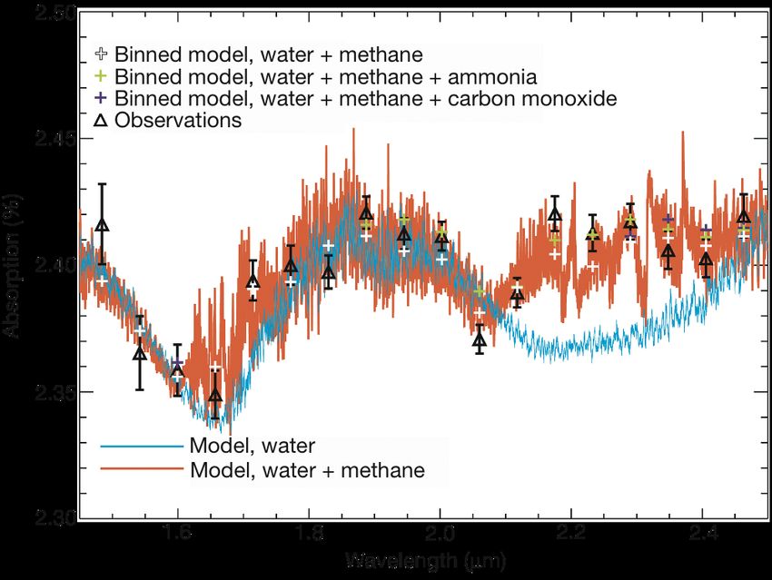
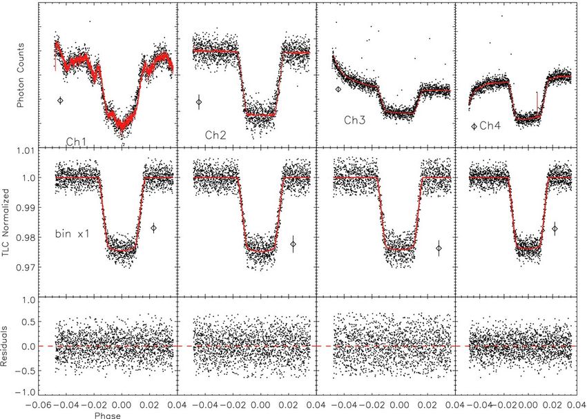
4

effects of molecules such as water vapor (Seager & Sasselov 1998; Marley et al. 1999;
Sudarsky, Burrows, & Pinto 2000; Barman, Hauschildt & Allard 2001), and borrowing
from brown dwarf observations and models (Oppenheimer et al. 1998). Work on cloud
modeling (Ackerman and Marley 2001; Cooper et al. 2003) and atmospheric circulation
(Showman & Guillot 2002; Cho et al. 2003) followed soon thereafter. Calculation of
exoplanet illumination phase curves, polarization curves (Seager, Whitney, & Sasselov
2000), and especially transmission spectra (Seager & Sasselov 2000; Brown 2001;
Hubbard et al. 2001) set the stage for observed spectroscopy during transit. Taken
together, this set of pioneering work built the foundation for the subsequent detection
and study of exoplanet atmospheres at that early time when theory was leading
observation.

In 2002, we and others began planning for secondary eclipse measurements of
transiting hot Jupiters using the Spitzer Space Telescope, launched in August 2003. At
mid-infrared wavelengths, hot Jupiters have a high planet-to-star contrast ratio, and the
star and planet typically are bright enough to allow high precision photon-limited
measurements. We expected to measure the planetary brightness temperature at
thermal wavelengths, as the planet disappeared and reemerged from behind the host
star. Coincidentally, other transiting planets were beginning to be found (Konacki et al.
2003). Although the first secondary eclipse detections (Charbonneau et al. 2005;
Deming et al. 2005a) were statistically robust at the just under 6-σ level, they again
were not absolutely convincing to the entire astronomy community. Any remaining
doubts, however, vanished with Spitzer's 16 µm secondary eclipse observation of HD
189733 (Deming et al. 2006). That measurement showed an obvious eclipse, with
amplitude 40 times the error level. This unleashed a flood of secondary eclipse
observational detections using Spitzer. Today we can count secondary eclipses of
about a dozen planets successfully observed by Spitzer at several wavelengths2, with
results published (Figure 1 and 2). An additional two dozen hot Jupiters have been
observed by Spitzer, with results under analysis, or have observations planned by
Warm Spitzer (see Table 1). It is accurate to say that no one anticipated the full
magnitude and stunning impact of the Spitzer Space Telescope as a tool to develop the
field of exoplanet atmospheric studies.

From its lonely beginnings just over a decade ago, the pendulum has swung to the point
where exoplanet atmospheric researchers now populate a full-fledged field, and have
produced over one hundred published papers. Today we can count atmospheric
observations of dozens of exoplanets, and particularly note observations of 8 especially
significant exoplanets (Figure 3). Skeptics are held at bay by the monumental and
pioneering achievements of the first decade of exoplanet atmospheric research. Indeed
the huge promise for the future is based on the incredible achievements of the past
decade. This review (as of January 2010) takes a critical, albeit not exhaustive, look at
the discoveries and future potential of exoplanet atmosphere studies.

2   http://ssc.spitzer.caltech.edu/approvdprog/
5

Figure 2. Collage of exoplanet atmosphere data and measurements. Most observed exoplanet
atmospheres are the four Spitzer/IRAC bands via secondary eclipse. For references see Table 1.
6

 Table 1. Spitzer IRAC Broad‐Band Photometry

10          3.6 µm           4.5 µm           5.8 µm           8 µm               Reference
                                                                                  Charbonneau et al.
HD189733b   0.256% ±0.014%   0.214% ±0.020%   0.310% ±0.034%   0.391 ±0.022%      2008
HD209458b   0.094% ±0.009%   0.213% ±0.015%   0.301% ±0.043%   0.240% ±0.026%     Knutson et al. 2008
                                                               0.084% +0.006% -
HD149026b   XX               XX               XX               0.012%             Harrington et al. 2007
                                                               0.0411% ±
                                                               0.0076%            Knutson et al. 2009c
HD80606b                     XX                                0.136% ±0.018%     Laughlin et al. 2009
GJ436b      XX               XX               XX               0.057% ± 0.008%    Deming et al. 2007
                                                               0.054% ± 0.007%    Demory et al. 2007
CoRoT-1     XX               XX
                             0.510% ±0.042
CoRoT-2     XX               %                                 0.41% ±0.11 %      Gillon et al. 2010
            0.080% ±         0.135% ±         0.203% ±
HAT-1       0.008%           0.022%           0.031%           0.238% ±0.040%     Todorov et al. 2010
HAT-2       X                X                XX               XX
HAT-3       X                X
HAT-4       X                X
HAT-5       XX               XX
HAT-6       X                X
                                                                                  Christiansen et al.
HAT-7       0.098% ±0.017%   0.159% ±0.022%   0.245% ±0.031%   0.225% ±0.052%     2010
HAT-8       X                XX
HAT-10      X                XX
HAT-11      X                X
HAT-12      X                X
                             0.066% ±                                             Charbonneau et al.
TrES-1      XX               0.013%           XX               0.225% ±0.036%     2005
            0.135% ±         0.245% ±         0.162% ±
TrES-2      0.036%           0.027%,          0.064%,          0.295% ±0.066%,    O’Donovan et al. 2010
            0.346%
TrES-3      ±0.035%          0.372% ±0.054%   0.449% ±0.097%   0.475% ±0.046%     Fressin et al. 2010
            0.137%
TrES-4      ±0.011%          0.148% ±0.016%   0.261% ±0.059%   0.318% ±0.044%     Knutson et al. 2009a
WASP-1      XX               XX               XX               XX
WASP-2      XX               XX               XX               XX
WASP-3      XX               XX                                XX
WASP-4      XX               XX
WASP-5      XX               X
WASP-6      XX               X
WASP-7      X                X
WASP-8                       XX                                XX
WASP-10     X                X
WASP-12     XX               XX               XX               XX
WASP-14     X                XX                                XX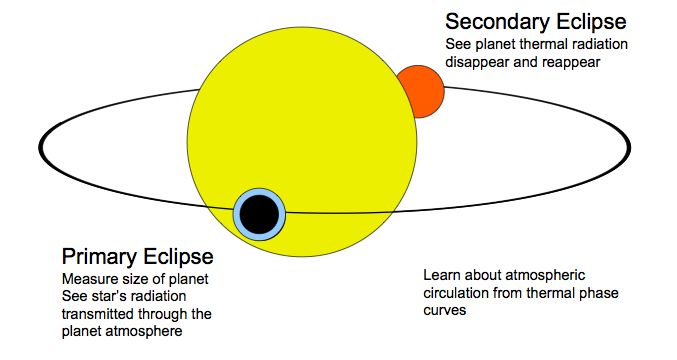
7
WASP-17 XX XX
WASP-18 XX XX XX XX
WASP-19 XX XX XX XX
XO-1 0.086% ±0.007% 0.122% ±0.009% 0.261% ±0.031% 0.210% ±0.029% Machalek et al. 2008
0.081% ± 0.098% ± 0.167% ±
XO-2 0.017% 0.020% 0.036% 0.133% ± 0.049% Machalek et al. 2009
XO-3 0.101% ±0.004% 0.143% ±0.006% 0.134% ±0.049% 0.150% ±0.036% Machalek et al. 2010
XO-4 XX X
Table 1. Tabulation of the exoplanet secondary eclipse observations. Reported values are published
measurements. A double x refers to data in hand and analyses under way. A single x refers to observations
officially planned by Spitzer as of January 2010. Wavelengths are in µm.
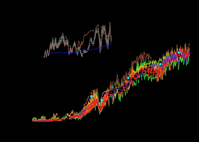
Figure 3. Panel illustrating Spitzer photometry for eight exoplanets including some of the most interesting
and significant exoplanets. Each sub‐panel has a different spatial scale, listed in AU below the planet name.
The Spitzer observational periods are indicated by colored arcs, with color indicating wavelength (see legend
at top). The very short arcs that appear similar to dots are short‐duration Spitzer observations. The spectral
type of the star (late‐F/G, K, or M) is indicated by color, and the stellar radii have been increased by a factor
of 3 for all systems, for greater visibility. Shading indicates the presence of a transit (lower shaded region),
or eclipse (upper shaded region). Our line of sight from Earth is from directly below each panel..8
2. Overview of Exoplanet Atmosphere Observations and Models
As a continued introduction we turn to background material for understanding exoplanet
atmosphere observations and models.
2.1 Observations
2.1.1 Direct Imaging
The most natural way to think of observing exoplanet atmospheres is by taking an
image of the exoplanet. This so-called “direct imaging” of planets is currently limited to
big, bright, young or massive planets located far from their stars (see Figure 1). Direct
imaging of substellar objects is currently
possible with large ground-based
telescopes and adaptive optics to cancel
the atmosphere's blurring effects. Out of a
dozen planet candidates, the most
definitive planet detections are Fomalhaut
b because of its mass (≤ 3 MJ) (Kalas et
al. 2008) and the three planets orbiting
HR 8799 (Marois et al. 2008). Not only do
the HR 8799 planets have mass
estimates below the brown dwarf limit, but
the hierarchy of three objects orbiting a
central star is simply not seen for multiple
star systems.
Figure 4. Black body flux (in units of 10‐26 W m‐2 Hz‐1)
Solar-system-like small exoplanets are not of some solar system bodies as “seen” from 10 pc.
observable via direct imaging with current The Sun is represented by a 5750 K black body. The
technology, even though an Earth at 10 pc planets Jupiter, Venus, Earth, and Mars are shown
and are labeled with their first initial. A putative hot
is brighter than the faintest galaxies Jupiter is labeled with “HJ”. The planets have two
observed by the Hubble Space Telescope peaks in their spectra. The short‐wavelength peak is
(HST). The major impediment to direct due to sunlight scattered from the planet atmosphere
imaging of exoEarths is instead the and is computed using the planet's geometric albedo.
The long‐wavelength peak is from the planet's
adjacent host star; the sun is 10 million to thermal emission and is estimated by a black body of
10 billion times brighter than Earth (for the planet's effective temperature. The hot Jupiter
mid-infrared and visible wavelengths, albedo was assumed to be 0.05 and the equilibrium
respectively). No existing or planned temperature to be 1600 K. Temperature and albedo
data was taken from Cox (2000).
telescope is capable of achieving this
contrast ratio at 1 AU separations. The
current state of the art HR 8799
observations detected a planet at a contrast of 1/100,000 at a separation of about 0.5
arcsec. Fortunately much research and technology development is ongoing to enable
space-based direct imaging of solar system aged Earths and Jupiters in the future. See9
Figure 4 for estimates of planetary fluxes, and Seager (2010; Chapter 3) for
approximate formulae for order of magnitude estimates for direct imaging.
2.1.2 Transiting Exoplanet Atmosphere Observations
For the present time, two fortuitous, related events have enabled observations of
exoplanet atmospheres using a technique very different from direct imaging. The first
event is the existence and discovery of a large population of planets orbiting very close
to their host stars. These so-called hot Jupiters, hot Neptunes, and hot super Earths
have up to about four-day orbits and semi-major axes less than 0.05 AU (see Figure 1).
The hot Jupiters are heated by their parent stars to temperatures of 1000 to 2000 K,
making their infrared brightness on the order of 1/1000 that of their parent stars (Figure
4). While it is by no means an easy task to observe a 1:1000 planet-star flux contrast,
such an observation is possible—and is unequivocally more favorable than the 10-10
visible-wavelength planet-star contrast for an Earth-twin orbiting a sun-like star.
The second favorable occurrence is that of transiting exoplanets—planets that pass in
front of their star as seen
from Earth. The closer the
planet is to the parent star,
the higher its probability to
transit. Hence the existence
of short-period planets has
enabled the discovery of
many transiting exoplanets.
It is the special transit
configuration that allows us
to observe the planet
atmosphere without imaging
Figure 5. Schematic of a transiting exoplanet and potential follow‐up
the planet.
measurements. Note that primary eclipse is also called a transit.
Transiting planets are
observed in the combined
light of the planet and star (Figure 5). As the planet passes in front of the star, the
starlight drops by the amount of the planet-to-star area ratio. If the size of the star is
known, the planet size can be determined. During transit, some of the starlight passes
through the the planetary atmosphere (depicted by the annulus in Figure 5), picking up
some of the spectral features in the planet atmosphere. A planetary transmission
spectrum can be obtained by dividing the spectrum of the star and planet during transit
by the spectrum of the star alone (the latter taken before or after transit).
Planets on circular orbits that pass in front of the star also disappear behind the star.
Just before the planet goes behind the star, the planet and star can be observed
together. When the planet disappears behind the star, the total flux from the planet-star
system drops because the planet no longer contributes. The drop is related to both10
relative sizes of the planet and star and their relative brightnesses (at a given
wavelength). The flux spectrum of the planet can be derived by subtracting the flux
spectrum of the star alone (during secondary eclipse) from the flux spectrum of both the
star and planet (just before and after secondary eclipse). The planet's flux gives
information on the planetary atmospheric composition and temperature gradient (at
infrared wavelengths) or albedo (at visible wavelengths).
Observations of transiting planets
provide direct measurements of the
planet by separating photons in time,
rather than in space as does imaging
(see Figure 5 and Figure 6). That is,
observations are made of the planet
and star together. (We do not favor the
“combined light” terminology because
ultimately the photons from the planet
and star must be separated in some
way. For transits and eclipses the
photons are separated in time.)
Primary and secondary eclipses
enable high-contrast measurements
because the precise on/off nature of
the transit and secondary eclipse
events provide an intrinsic calibration
reference. This is one reason why the Figure 6 Infrared light curve of HD 189733A and b at 8 µm.
The flux in this light curve is from the star and planet
HST and the Spitzer Space Telescope
combined. Panel a: the first dip (from left to right) is the
(Spitzer) have been so successful in transit and the second dip is the secondary eclipse. Panel b:
measuring high-contrast transit signals a zoom in of panel a. Error bars have been suppressed for
that were not considered in their clarity. Data from Knutson et al. (2007a).
designs.
2.2 Atmosphere Models and Theory
A range of models are used to predict and interpret exoplanet atmospheres. Usage of a
hierarchy of models is always recommended. Interpreting observations and explaining
simple physical phenomena with the most basic model that captures the relevant
physics often lends the most support to an interpretation argument. More detailed and
complex models can further support results from the more basic models. The material in
this subsection is taken from Seager (2010).
Computing a model spectrum. The equation of radiative transfer is the foundation not
only to generating a theoretical spectrum but also to atmosphere theory and models.
The radiative transfer equation is the change in a beam of intensity dI/dz that is equal to
losses from the beam –κI and gains to the beam ε, and the 1D plane-parallel form is11
Here: I is the intensity [Jm-2s-1Hz-1sr-1], a beam of traveling photons; κ is the absorption
coefficient [m-1] which includes both absorption and scattering out of the radiation beam;
ε is the emission coefficient [Jm-3s-1Hz-1sr-1] which includes emission and scattering into
the beam; µ = cos θ, where θ is the angle away from surface normal; and z is vertical
altitude, where each altitude layer has a specified temperature and pressure. Using the
definition of optical depth τ, , yields a common form of the radiative transfer
equation,
.
Here we have omitted scattering, adopted LTE, and used Kirchoffʼs law B = ε/κ, to
explicitly use the blackbody function B.
The solution of the radiative transfer equation has a long history in stellar and planetary
atmosphere theory. Simplified solutions for exoplanet spectra are possible for:
transmission spectra by the case of no emission (i.e., ε = 0); and for atmospheric
thermal emission spectra by ignoring scattering in the κ and ε terms. The significant
differences in radiative transfer between exoplanet atmospheres and stellar
atmospheres are the boundary condition at the top of the atmosphere, namely the
incident stellar radiation, and the possibility of clouds for exoplanet atmospheres.
Inherent in the radiative transfer equation are opacity, chemistry, and clouds, via the
absorption coefficient κ and the emission coefficient ε. It is fair to say that almost all of
the detailed physics and the unknowns are hidden in these macroscopic coefficients.
The absorption coefficient for a single gas species is defined by κ(λ,T, P) = n(T,P)σ(λ,T,
P), where n is the gas number density, and σ(λ,T, P) is the cross section summed over
all molecular lines that contribute at a given wavelength and that includes partition
functions. At a given wavelength, κ from all relevant gas molecules must be included.
The cross sections themselves come from either laboratory measurements or from
quantum mechanics calculations. For a description of opacity calculations relevant to
exoplanets see Freedman, Marley, & Lodders (2008), Sharp & Burrows (2007), and the
HITRAN database (Rothman et al. 2009).
The number density of a gas molecule can be calculated from equilibrium chemistry
(e.g., Burrows & Sharp 1999; Lodders & Fegley 2002). In some cases, nonequilibrium
chemistry is significant, especially for situations where the strong CO double bond and
N2 triple bond cannot be broken fast enough to reach chemical equilibrium (e.g.,
Saumon et al. 2006). Photochemistry is significant in driving the molecular abundances
for low-mass rocky planets with thin atmospheres. Such planets cannot hold onto the
light chemical species and do not have deep atmosphere temperatures and pressures
to return photochemical products back to their equilibrium concentrations. Atmospheric
escape is a further complication for the outcome of low-mass and/or hot exoplanet
atmosphere composition and determines which elements remain in the atmosphere.12 Clouds complicate the radiative transfer solution due to the often high opacity of solid material. The type of cloud that forms depends on the condensation temperature of the gas, and for hot Jupiters high-temperature condensates such as iron and silicates are likely present. For an excellent introduction to cloud physics see Sanchez-Lavega, Perez-Hoyos, & Hueso (2004). Given an atmospheric temperature-pressure profile, a planetʼs emergent spectrum can be calculated with all of the above ingredients. In exoplanet atmospheres, a reality check comes from the idiom “what you put in is what you get out”. This is a warning that arbitrary choices in inputs (molecular abundances and boundary conditions) can control the output spectrum. Computing a 1D temperature profile: radiative transfer, hydrostatic equilibrium and conservation of energy. In order to describe the temperature-pressure structure of a planetary atmosphere, three equations are needed. The equation of radiative transfer, the equation of hydrostatic equilibrium, and the equation of conservation of energy. With these three equations, three unknowns can be derived: temperature as a function of altitude; pressure as a function of altitude; and the radiation field as a function of altitude and wavelength. Hydrostatic equilibrium describes how the atmospheric pressure holds up the atmosphere against gravity, and relates pressure to altitude. Conservation of energy is described by radiative equilbrium in an altitude layer: energy is conserved because energy is neither created nor destroyed in the atmosphere. If the atmosphere layer(s) is unstable against convection, then convective equilibrium or radiative-convective equilibrium holds and is used to describe energy transportation in that layer. All of the chemistry, opacity, and cloud issues hold for the computation of the vertical temperature profile of a planet atmosphere because heating and cooling depends on the details of absorption and emission at different altitudes. Computing the 3D atmospheric structure: atmospheric circulation Atmospheric circulation is the large-scale movement of gas in a planetary atmosphere that is responsible for distributing energy absorbed from the star throughout the planetary atmosphere. The best current example where atmospheric circulation models are required are hot Jupiter exoplanets. With semi-major axes less than about 0.05 AU, hot Jupiters are expected to be tidally-locked to their host stars, having a permanent day and night side. Furthermore, because of the close stellar proximity, the planetary dayside is intensely irradiated by the host star, setting up a radiative forcing regime not seen in the solar system. An understanding of both the emergent spectra (e.g., Fortney et al. 2006) and the redistribution of absorbed stellar energy (e.g., Showman, Cho, & Menou 2010) require atmospheric circulation models. Atmospheric circulation models are based on the fluid dynamic equations. They come from six fundamental equations: the conservation of mass, conservation of momentum (one equation for each dimension), conservation of energy, and the ideal gas law as the
13

equation of state. Some investigators have used the full set of equations for exoplanet
models. Others take the traditional planetary atmospheres approach resulting from four
decades of study: the primitive equations. The primitive equations replace the vertical
momentum equation with local hydrostatic balance, thereby dropping the vertical
acceleration, advection, Coriolis, and metric terms that are generally expected to be less
important for the global-scale circulation, such that energy is still conserved. Still other
researchers use a 2D version, the shallow water equations. Because of the short
timescales involved for radiation transport, atmospheric circulation models traditionally
use very elementary radiation schemes that might not be suitable for hot Jupiters. This
is recently changing as radiative transfer schemes are implemented (Showman et al.
2009; Menou & Rauscher 2009). The limiting factors of atmospheric circulation research
are both the nonlinearity of the equations and the very computationally intensive
models.

Atmospheric circulation is not always necessary to compute spectra for many types of
planets (e.g., equatorially-viewed Earth, Jupiter), especially given the current quality of
exoplanet data. Atmospheric circulation, however, is needed to understand planets with
strong external radiative forcing. In addition, atmospheric circulation partly controls
surface temperatures and drives large-scale cloud patterns (and hence albedo) on
terrestrial planets. See Showman, Cho, & Menou (2010) for a description of all of these
ideas as well as applications to both giant and terrestrial planets.

2.3 Anticipated Planet Atmosphere Diversity
The diversity of planet interior
compositions is highly relevant to
atmospheres, so we show in Figure
7 a generic summary of types of
exoplanets via their bulk
composition as a function of rock,
ice, or gas components (Chambers
2010, Rogers & Seager 2009; see
Seager et al. 2007 for a description
of mass-radius relations for planet
interior compositions).
                                       Figure 7. Schematic diagram illustrating the range of
In the solar system there is a         possible planet primordial bulk compositions for
definite relationship between the      exoplanets. In this figure “gas” refers to primordial H and
relative abundances of rock-ice-gas    He accreted from the nebula, “ice” refers to ice‐ forming
                                       materials, and “rock” refers to refractory materials.
and planet mass: small planets (M      Constraints on the current compositions of the solar
≤ 1 M⊕) are rocky, intermediate        system planets are plotted in purple (planets are denoted
planets (~15-17 M⊕) are icy, and       by their first initial). Exoplanets might appear anywhere in
larger planets are predominantly       this diagram. Adapted from Chambers (2010) and Rogers
                                       and Seager (2009).
composed of H and He. Whether or
                                       Figure 1. Known exoplanets. Note that no existing
                                       program can discover Earth analogs. The phase space
                                       covered by ExoplanetSat extends as low as 1 Earth mass,
                                       and out to 1 AU.
14
not exoplanets also follow this pattern is one of the most significant questions of
exoplanet formation, migration and evolution.
Exoplanet atmospheres are related to their interiors, but how much so remains an
outstanding question. The best way to categorize exoplanet atmospheres in advance of
detailed observations is within a framework of atmospheric content based on the
presence or absence of volatiles (see Rogers and Seager for a discussion focusing on a
specific exoplanet, GJ 1214b). We choose five categories of atmospheres:
1. Dominated by H and He. Planetary atmospheres that predominately contain both
H and He, in approximately cosmic proportions are atmospheres indicative of
capture from the protoplanetary nebula (or planet formation from gravitational
collapse). In our solar system these include the giant and ice giant planets
2. Outgassed atmospheres with H. Planets that have atmospheres from outgassing
and not captured from the nebular disk will have some hydrogen content in the
form of H2. How much depends on the composition of planetesimals from which
the planet formed (Elkins-Tanton & Seager 2008; Schaefer and Fegley 2010).
The idea is that some planets in the mass range 10 to 30 Earth masses will be
massive enough and cold enough to retain hydrogen in their atmospheres
against atmospheric escape. Such H-rich atmospheres will have a different set of
dominating molecules (H2, naturally occurring H2O, and CH4 or CO) as compared
to solar system terrestrial planets with CO2 or N2 dominated atmospheres. Some
super Earths may have outgassed thick atmospheres of up to 50% by mass of H,
up to a few percent of the planet mass. Other planets may have massive water
vapor atmospheres (e.g., Leger et al. 2004; Rogers & Seager 2009). Outgassed
atmospheres will not have He, since He is not trapped in rocks and cannot be
accreted during terrestrial planet formation (Elkins-Tanton and Seager 2008).
3. Outgassed atmospheres dominated by CO2. On Earth CO2 dissolved in the
ocean and became sequestered in limestone sedimentary rocks, leaving N2 as
the dominant atmospheric gas. This third category of atmospheres, stemming
from either the first or second category, is populated by atmospheres that have
lost hydrogen and helium, wherein signs of H2O will be indicative of a liquid water
ocean. The actual planet atmospheric composition via outgassing depends on
the interior composition.
4. Hot super Earth atmospheres lacking volatiles. With atmospheric temperatures
well over 1500 K, hot Earths or super Earths will have lost not only hydrogen but
also other volatiles such as C, N, O, S. The atmosphere would then be
composed of silicates enriched in more refractory elements such as Ca, Al, Ti
(Schaefer & Fegley 2009).15
5. Atmosphereless planets. A fifth and final category are hot planets that have lost
their atmospheres entirely. Such planets may have a negligible exosphere, like
Mercury and the Moon. Transiting planets lacking atmospheres can be identified
by a substellar point hotspot (e.g., Seager & Deming 2009); for planets with
atmospheres the hot spot is likely to be advected from the substellar point and for
planets with thick atmospheres the planet might not be tidally locked.
The actual atmospheric molecular details of the above scenarios must await theoretical
calculations that include outgassing models, photochemistry calculations, atmospheric
escape computations, and also future observations. Understanding enough detail to
create such a classification scheme may well occupy the field of exoplanet atmospheres
for decades to come.
At the present time there is a great divide between the hot Jupiter exoplanets that we
can study observationally and the super Earths that we want to study but which are not
yet accessible. We begin with observation and interpretation highlights of hot Jupiters.
3. Discovery Highlights
We now turn to a summary of the most significant exoplanet atmospheric discoveries.
Hot Jupiters dominate exoplanet atmosphere science, because their large radii and
extended atmospheric scale heights facilitate atmospheric measurements to maximum
signal-to-noise. Even so, data for hot Jupiters remain limited, so their physical picture
cannot yet be certainly described. We here address what we have learned from the
observations alone, as well as from interpreting the observations with the help of
models. In so doing, we rely on the formal uncertainties of each observation as
reported in the literature. We discuss these conclusions starting with the most robust,
and working toward more tentative results.
3.1. Hot Jupiters are Hot and Dark
Hot Jupiters are blasted with radiation from the host star. They should therefore be
kinetically hot, heated externally by the stellar irradiance. Indeed, early hot Jupiter
model atmospheres already predicted temperatures exceeding 1000K (Seager &
Sasselov 1998; Sudarsky, Burrows, & Hubeny 2003). The first and most basic
conclusion from the Spitzer secondary eclipse detections (e.g., Figure 6) was the
confirmation of this basic paradigm. The fact that the planets emit generously in the
infrared implies that they efficiently absorb visible light from their stars. Searches for the
reflected component of their energy budget have indicated that the planets must be very
dark in visible light, with geometric albedos less than about 0.2 (Rowe et al. 2008), and
likely much lower. Purely gaseous atmospheres lacking reflective clouds can be very
dark (Marley et al. 1999; Seager, Whitney, & Sasselov 2000) but HD209458b also
requires a high-altitude absorbing layer (see below) to account for its atmospheric
temperature structure.16
3.2 Identification of Atoms and Molecules
A planetary atmosphere with elemental
composition close to solar and heated
upwards of 1000 K is expected to be
dominated by the molecules H2, H2O,
and, depending on the temperature
and metallicity, CO and/or CH4. Of
these molecules, H2O is by far the
most spectroscopically active gas.
Water vapor is therefore expected to
be the most significant spectral feature
in a hot Jupiter atmosphere. Some
initial indications from Spitzer
spectroscopy that water absorption
Figure 8. Transmission spectrum of the transiting planet
was absent (Richardson et al. 2007; HD 189733. Hubble Space Telescope observations shown
Grillmair et al. 2007) were superceded by the black triangles. Two different models highlight the
by higher S/N data that clearly showed presence of methane in the planetary atmosphere. From
water absorption (Grillmair et al. 2008; Swain et al. (2008).
Swain et al. 2008, Swain et al 2009a).
See Figures 8 and 9.
Other atoms and molecules identified in hot Jupiter atmospheres are atomic sodium
(Na) (e.g., Charbonneau et al. 2002; Redfield et al. 2008), methane (CH4) (Swain et al.
2008), carbon monoxide (CO), and carbon dioxide (CO2) (e.g., Swain et al. 2009a,b;
Madhusudhan and Seager 2009). This set of molecules has been detected in the two
hot Jupiters most favorable for observation (HD 209458b and HD 189733b). It is
instructive to consider which atomic and molecular identifications are model-
independent and which depend on models. The atomic sodium detections are
independent of models, because there is no other plausible absorber at the sodium-
doublet wavelength (see the analysis in Charbonneau et al. 2002). The HST
spectrophotometry has sufficiently high spectral resolution to show distinct features from
H2O, CH4, and CO2. Those detections may also be considered model-independent
because they rely only on molecular absorption cross section information.
Planets with host stars fainter than approximately V=8 have been observed primarily
using broad-band photometry, since they do not produce enough photons to be
observed to the requisite precision with HST/NICMOS or the Spitzer/IRS instrument.
From broad-band photometry, not only are model fits needed to identify molecules, but
some assumptions as to which spectroscopically active molecules are present is
essential. Taking H2O, CH4, CO and CO2 as the molecules with features in the Spitzer
3.5-24 µm range, molecular identification is possible for H2O and CH4 from the four17 Spitzer/IRAC bandpasses between 3.4 and 8 µm and for H2O, CH4, CO and CO2 with the additional Spitzer/IRS 16 µm Spitzer/MIPS 24 µm bandpass (see Figure 9). Figure 9. Thermal emission data composite for HD 189733 in secondary eclipse. Data from HST/NICMOS (inset: Swain et al. 2009), Spitzer/IRAC (four shortest wavelength red points; Charbonneau et al. 2008), Spitzer/IRS‐PU (Deming et al. 2006), Spitzer/MIPS (Charbonneau et al. 2008), Spitzer/IRS (black points from 5 – 13 microns; Grillmair et al. 2008). Models shown in the bottom panel (from Madhusudhan and Seager 2009) illustrate that the best fits to the Spitzer/IRS ((red curve shows fits within the 1.4σ errors, on average; orange 1.7σ, green 2σ, and blue is one best fit model within 1.4σ) and Spitzer photometry (brown curve within 1σ) do not fit the NICMOS data (inset grey curves within 1.4σ) possibly implying variability in the planet atmosphere from data taken at different epochs. For abundance constraints from the difference models, see Madhusudan and Seager (2009). A thorough temperature and abundance retrieval method enables statistical constraints on molecular mixing ratios and other atmospheric properties (e.g., Madhusudhan and Seager, 2009). As a best case example, the HST/NICMOS spectrum of 189733b at secondary eclipse yields constraints of H2O ~ 10-4, considering fits within the ~ 1.5 σ observational uncertainties. For other species and other data sets, the constraints are not nearly as good. At the same level of fit, the six-channel Spitzer photometry of HD 209458b at secondary eclipse yields constraints of H2O < 10-4, CH4 > 10-8, CO > 4 x 10- 5 , and 2 x 10⁻⁹ < CO2 < 7 x 10⁻⁶. The constraints placed to date have been limited by the number of simultaneous broadband observations available, which are typically fewer than the number of model parameters. The inference of CO2 is interesting, because a planetary atmosphere dominated by molecular hydrogen is expected to have CO or CH4 as the primary reservoir of carbon at high temperatures. For a hot atmosphere with CO as the primary carbon reservoir, CO2 could be reasonably abundant ~10-6, based on thermochemistry (Lodders & Fegley 2002) or photochemistry (Liang et al. 2003), but higher values require a high planet metallicity (Zahnle et al. 2009). CO2 mixing ratios of 10-4 or higher might be needed to explain the observed CO2 features in the HST/NICMOS dataset for the HD 189733 thermal emission spectrum (Madhusudhan and Seager 2009; c.f. Swain et al. 2009a). In addition to molecules, the presence of atmospheric haze has been inferred in HD 189733 via transmission spectra with HST/STIS. While the particle composition has not been identified, the Rayleigh-scattering behavior of the data indicates small particle
18

sizes (Pont et al. 2008). The presence of haze on HD189733b is consistent with similar
inferences for HD209458b. In the latter planet, high clouds or haze have been invoked
to account for the weakness of the sodium absorption (Charbonneau et al. 2002), and
the upper limits on CO absorption (Deming et al. 2005b), during transit.

3.3 Day-Night Temperature Gradients
Hot Jupiters are fascinating fluid dynamics laboratories because they probably have a
permanent dayside and a permanent night side. Close-in giant planets are theorized to
have their rotation synchronized with their orbital motion by tidal forces, a process that
should conclude within millions of years (e.g., Guillot et al. 1996). Under this tidal-
locking condition the planet will keep one hemisphere perpetually pointed toward the
star, with the opposite hemisphere perpetually in darkness.

A resulting key question about tidally-locked hot Jupiters concerns whether one side of
the planet is extremely hot, and the other side remains very cold. Or does atmospheric
circulation even out the planetary day to night side temperature difference?
Observational evidence exists for planets approaching both extremes. Spitzer thermal
infrared observations of HD 189733b show that the planet has only a moderate
temperature variation from the day to night side. The planet shows an 8 µm brightness
temperature variation of over 200 K from a minimum brightness temperature of
973±33K to a maximum brightness temperature of 1212±11K (Knutson et al. 2007a),
and a thermal brightness change at 24 µm consistent with the 8 µm data within the
errors (Knutson et al. 2009c). In contrast to HD 189733b, Ups And and HAT-P-7 show a
dramatic change in thermal brightness from the day to the night side. Although the Ups
And data are not continuous, the brightness change at 8 µm measured with Spitzer
indicates a temperature change of well over 1000 K. HAT-P-7b, with a dayside
equilibrium temperature above 2,000 K, has a spectacular phase curve measured by
the Kepler Space Telescope (Borucki et al. 2010). The HAT-P-7b data are difficult to
interpret in terms of day-night temperature gradient because Keplerʼs single broad
bandpass (from 420 to 900 nm) allows both thermal emission and reflected radiation to
contribute to the observed signal, and because visible-wavelength thermal emission at
the Wien tail changes rapidly for a ~2,000 K black body radiator decreasing in
temperature.

A word of caution is warranted concerning the day-night temperature gradient inferred
from broad-band photometric light curves. One could imagine a malevolent situation
where an emission band present on the planetary dayside turns into an absorption
feature on the planetary night side. This scenario would mimic a large horizontal thermal
gradient but would actually be caused by a variation in vertical temperature gradient,
without the need for significant day-night temperature differences.

One particularly interesting result that is relevant to day-night temperature differences is
Spitzer's observation of the periastron passage of the very eccentric (e=0.93) planet
HD80606b (Laughlin et al. 2009). Radiative cooling plays a role in day-night
19

temperature differences, and Spitzer's observed time-dependent heating of this planet
at periastron constrains the atmospheric radiative time constant. Moreover, because
rotation modulates the flux we receive from the sub-stellar hemisphere at periastron,
those observations also provide key information on the planet's pseudo-synchronous
rotation. The pseudo-synchronous rotation rate in turn is sensitive to the physics of
energy dissipation in the planetary interior. So Spitzer observations of eccentric planets
can in principle provide information on planetary interiors as well as atmospheres.

Turning to model interpretation of the planet HD 189733b, Spitzer thermal emission light
curve observations indicate that strong winds have advected the hottest region to the
east of the sub-stellar point (Knutson et al. 2007a; Showman et al. 2009). The shifted
hot region on the dayside carries physical information such as the speed of the zonal
circulation, and information about the altitude and opacity-dependence of the
atmospheric radiative time constant.

Theory alone can articulate a few significant points about atmospheric circulation. Giant
planets in our solar system also have strong zonal winds, appearing in multiple bands at
different latitudes. Consideration of the relatively slow rotation rate of hot Jupiters
(probably equal to their orbital period of a few days) leads us to believe that their zonal
winds will occur predominantly in one or two major jets that are quite extended in
latitude and longitude (e.g., Showman & Guillot 2002; Menou et al. 2003). The relatively
large spatial scale of hot Jupiter winds—and the corresponding temperature field—
should be a boon to their observational characterization. Planets with temperature
fluctuations only on small scales will have little to no variation in the amount of their
hemisphere-averaged flux as a function of orbital phase. Atmospheric circulation models
also show that it seems likely that at least some hot Jupiters transport energy
horizontally via zonal winds having speeds comparable to the speed of sound (e.g.,
Showman et al. 2010).

3.4 Atmospheric Escape
Escaping atomic hydrogen from the exosphere of the hot Jupiter HD 209458b has been
detected during transit in the Ly α line. A positive detection was made with HST/STIS
(3.75 σ) HST/STIS (Vidal-Madjar et al. 2003). (Other absorption features claimed at
lower statistical significance are not discussed here.) Showing a 15% drop in stellar Ly
α intensity during transit, the HD 209458b observations are interpreted as a large cloud
of hot hydrogen surrounding the planet. The cloud extends up to 4 planetary radii, and
the kinetic temperature is as high as tens of thousands of K. It extends beyond the
planetary Roche lobe, so the hydrogen is evidently escaping to form a possible comet-
like coma surrounding the planet. Models agree that the implied exospheric heating is
likely due to absorption of UV stellar flux, but Jeans escape is not sufficient to account
for the hydrogen cloud. The specific origin of the escaping atoms is model-dependent.
Escape mechanisms include radiation pressure, charge exchange, and solar wind
interaction (see, e.g. Lammer et al. 2009 and references therein).
20
3.5 Vertical Thermal Inversions
Almost all solar system planets have thermal inversions high in their atmospheres (i.e.,
the temperature is rising with height above the surface). These so-called stratospheres
are due to absorption of UV solar radiation by CH4 -induced hazes or O3. Thermal
inversions in hot Jupiter atmospheres were not widely predicted, because of the
expected absence of CH4, hydrocarbon hazes, and O3.
Evidence for vertical atmospheric thermal inversions in hot Jupiters comes from
emission features in place of (or together with) absorption features in the thermal
infrared spectrum (for a basic explanation see Seager 2010). Because broad-band
photometry does not delineate the structure of molecular spectral bands, the inference
of a thermal inversion must rely on models. Moreover, the presence of specific
molecules must be inferred based on the anticipated physical conditions, guided by
models. Spitzer data show that the upper atmospheres of several planets have thermal
inversions, if water vapor is present and if abundances are close to solar (e.g., Burrows
et al. 2008; see Figure 10).
The hot Jupiter temperature
inversions are likely fueled by
absorption of stellar irradiance in a
high-altitude absorbing layer.
Possibilities for a high-altitude
absorber include gaseous TiO and
VO (Hubeny, Burrows, & Sudarsky
2003; Fortney et al. 2007), as well
as possibilities involving
photochemical hazes (Zahnle et al.
2009). Under a simple irradiation-
driven scenario, the stronger the
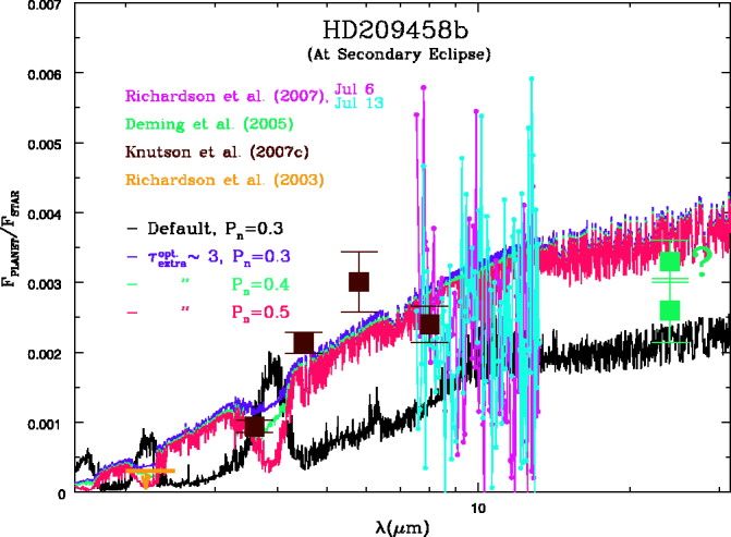
stellar irradiance, the more likely Figure 10. Evidence for an atmospheric thermal inversion for
that an inversion would occur HD 209458b. Spitzer data points from secondary eclipse
(Hubeny, Burrows, & Sudarsky measurements are shown with brown (IRAC; Knutson et al.
2003; Fortney et al. 2007; Burrows, 2007) and green (Deming et al. 2005 and private comm.; the
two points are data taken at different times). IRS spectra
Hubeny, Budaj 2008). In addition, shown in purple and aqua are from Richardson et al. (2007).
under this irradiation-driven The model in pink shows emission features from an
scenario, planets with strong atmospheric thermal inversion. The black curve is a non‐
thermal inversions are also thermal‐inversion model. Figure from Burrows et al. (2007).
expected to show strong day-night
temperature gradients. Hot Jupiters are probably more complex than this simple
division allows; HD 189733b and XO-1b have virtually identical levels of irradiation and
yet XO-1b appears to have an inversion (Machalek et al. 2008) while HD 189733b does21 not (Charbonneau et al. 2008). So it is possible that not-yet-understood chemistry may be a more dominant factor than stellar irradiance. Taking a critical look at the evidence for thermal inversions, (Madhusudhan & Seager (2010)) found that for many cases existing observations (Spitzer broad-band photometry) are not enough to make robust claims on the presence of thermal inversions. For some of these cases, the observations can be explained without thermal inversions, along with rather plausible chemical compositions. For other cases, the observations can be explained by models without thermal inversions if the models have a high abundance of CH4 instead of CO. The dominance of methane as the carbon- bearing molecule would indicate severe non-equilibrium chemistry, since at high temperatures CO is the most stable, and hence most abundant, carbon-bearing molecule. 3D atmospheric circulation models also have difficulty explaining the Spitzer IRAC data of HD 209458b and other planets with purported thermal inversions (Showman et al. 2009). The models produce day-night redistribution over a continuous range of pressures; as a result the circulation models produce temperature profiles that do not explain the IRAC data, even if a thermal inversion is present at some locations (Showman et al. 2009). Determination of thermal inversions will be more solid and less model-dependent and degenerate when higher spectral resolution and higher S/N observations become available using JWST, or possibly advanced ground-based facilities. 3.6 Variability Variability in the hot Jupiter atmospheric data is relatively common at the 2σ level. While this would not be statistically significant in a particular case, it is highly suggestive in the aggregate, because it occurs more frequently than is expected based on statistical error distributions. A possible mundane explanation is that the observers have underestimated their statistical errors. Nevertheless, many observers use careful methods for error estimation, so we must consider the intriguing possibility that the atmospheres of hot Jupiters are intrinsically variable to a significant degree. Moreover, there are some specific examples where variability seems inescapable, unless there are major systematic errors in the observations. For example, the CO2 feature detected in HD189733b at 2.3 µm with HST/NICMOS during both transit (Swain et al. 2008) and eclipse (Swain et al. 2009) is far too strong to be consistent with the lack of an observed CO2 absorption at 4 µm and 16 µm in secondary eclipse observations (Charbonneau et al. 2008). The CO2 absorption cross sections are much greater at 4- and 16- than at 2.3 µm, so this conclusion is not significantly model-dependent (see Madhusudhan and Seager 2009).
22

4 Observational Challenges for Transiting Planet Observations

Hand-in-hand with the exoplanet atmosphere discovery highlights based on
observations are issues of systematic effect removal. The HST and Spitzer were not
designed to achieve the very high signal-to-noise ratios necessary to study transiting
exoplanets, but they have succeeded nonetheless. We have learned from these
observations that with enough photons, systematics that were unknown in advance can
often be corrected, as long as the time scale and nature of the systematic effects do not
overlap too strongly with the time scale of the signals being sought. A cautionary view
is that observers are pushing the limit of telescopes and instruments far past their
design specifications. The art and science of exoplanet atmospheric observations,
therefore, is instrument systematic removal to extract a planetary atmospheric signal.
Extreme care must be taken to reach realistic results and to assign appropriate error
limits.

4.1 Systematic Observational Errors and Their Removal
Separating the light of exoplanets from that of their star is difficult. The contrast ratio
(planet divided by star) is greater in the infrared than in the optical, but it can still be as
small as 10-4, or even less (Figure 4). Because transit and eclipse methods reply on
separating the planetary and stellar light in the time domain, we have to be concerned
with the temporal stability of the measurements at the 10-4 level or less. Also,
astronomers want to push the measurements to increasingly smaller planets, that have
even lower planet-star contrast ratios than the currently-studied hot Jupiters. Inevitably,
then, we are going to have to deal with systematic observational errors caused by
temporal instabilities. Even for hot, giant exoplanets, these systematic errors are
already a significant issue.

Systematic errors are not random, they are signals in their own right. The key to their
removal is in understanding the origin and nature of those signals, so that they can be
modeled and removed from the data, leaving the planetary signal undistorted by the
process. Nearly all of the facilities that have measured light from exoplanets are
general purpose: HST, Spitzer, and ground-based observatories. NASAʼs Kepler Space
Telescope is an exception to the general purpose telescope in that Kepler was
specifically designed to acquire stable, precise stellar photometry. See Caldwell et al.
(2010) for a report on Kepler systematics. Most other facilities, however, have some
sources of systematic error in common, such as pointing instabilities, but the details
differ with the specific telescope/instrument/detector and observing methodology.

4.1.1 Spitzer
Spitzer is among the most widely-used facilities for exoplanet characterization and so its
systematic effects make particularly good examples. Overall, Spitzer is remarkably
stable due to its cryogenic state and its placement in the thermally stable environment of
heliocentric orbit. Also minimizing Spitzer systematics is the fact that the Spitzer
instruments have very few moving parts. Spitzer results have therefore overall been
You can also read