COSMIC RAYS AND CLIMATE - EUROPEAN ORGANIZATION FOR NUCLEAR RESEARCH
←
→
Page content transcription
If your browser does not render page correctly, please read the page content below
EUROPEAN ORGANIZATION FOR NUCLEAR RESEARCH

                                                                         CERN-PH-EP/2008-005
                                                                               26 March 2008

                          COSMIC RAYS AND CLIMATE

                                       Jasper Kirkby
                                CERN, Geneva, Switzerland

                                          Abstract
Among the most puzzling questions in climate change is that of solar-climate variability,
which has attracted the attention of scientists for more than two centuries. Until recently,
even the existence of solar-climate variability has been controversial—perhaps because
the observations had largely involved correlations between climate and the sunspot cycle
that had persisted for only a few decades. Over the last few years, however, diverse
reconstructions of past climate change have revealed clear associations with cosmic ray
variations recorded in cosmogenic isotope archives, providing persuasive evidence for
solar or cosmic ray forcing of the climate. However, despite the increasing evidence of
its importance, solar-climate variability is likely to remain controversial until a physical
mechanism is established. Although this remains a mystery, observations suggest that
cloud cover may be influenced by cosmic rays, which are modulated by the solar wind
and, on longer time scales, by the geomagnetic field and by the galactic environment of
Earth. Two different classes of microphysical mechanisms have been proposed to connect
cosmic rays with clouds: firstly, an influence of cosmic rays on the production of cloud
condensation nuclei and, secondly, an influence of cosmic rays on the global electrical
circuit in the atmosphere and, in turn, on ice nucleation and other cloud microphysical
processes. Considerable progress on understanding ion-aerosol-cloud processes has been
made in recent years, and the results are suggestive of a physically-plausible link between
cosmic rays, clouds and climate. However, a concerted effort is now required to carry out
definitive laboratory measurements of the fundamental physical and chemical processes
involved, and to evaluate their climatic significance with dedicated field observations and
modelling studies.

Keywords
aerosols, clouds, climate, solar-climate variability, cosmic rays, ions, global electrical cir-
cuit, CERN CLOUD facility

                                      Published in
      Surveys in Geophysics 28, 333–375, doi: 10.1007/s10712-008-9030-6 (2007).
             The original publication is available at www.springerlink.com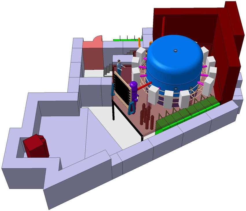
Contents

1   INTRODUCTION                                                                                             1

2   SOLAR/COSMIC RAY-CLIMATE VARIABILITY                                                                     2
    2.1   Last millennium . . . . . . . . . . . . . . . . . . . . . . . . . . . . . . . . . . . . . . .      2
          2.1.1   The Little Ice Age and Medieval Warm Period . . . . . . . . . . . . . . . . . .            2
          2.1.2   Intertropical Convergence Zone . . . . . . . . . . . . . . . . . . . . . . . . . .         4
          2.1.3   Solar and cosmic ray changes since the Little Ice Age . . . . . . . . . . . . . . .        5
    2.2   Holocene; last 10 ky . . . . . . . . . . . . . . . . . . . . . . . . . . . . . . . . . . . .       8
          2.2.1   Ice-rafted debris in the North Atlantic Ocean . . . . . . . . . . . . . . . . . . .        8
          2.2.2   Indian Ocean monsoon . . . . . . . . . . . . . . . . . . . . . . . . . . . . . . .         9
    2.3   Quaternary; last 3 My . . . . . . . . . . . . . . . . . . . . . . . . . . . . . . . . . . . .     10
          2.3.1   Stalagmite growth in Oman and Austria . . . . . . . . . . . . . . . . . . . . . .         10
          2.3.2   Laschamp event . . . . . . . . . . . . . . . . . . . . . . . . . . . . . . . . . . .      12
    2.4   Phanerozoic; last 550 My . . . . . . . . . . . . . . . . . . . . . . . . . . . . . . . . . .      13
          2.4.1   Celestial cycles . . . . . . . . . . . . . . . . . . . . . . . . . . . . . . . . . . .    13
          2.4.2   Biodiversity . . . . . . . . . . . . . . . . . . . . . . . . . . . . . . . . . . . . .    14

3   MECHANISMS                                                                                              15
    3.1   GCR-cloud mechanisms . . . . . . . . . . . . . . . . . . . . . . . . . . . . . . . . . .          15
          3.1.1   GCR characteristics . . . . . . . . . . . . . . . . . . . . . . . . . . . . . . . .       15
          3.1.2   Ion-induced nucleation of new aerosols . . . . . . . . . . . . . . . . . . . . . .        15
          3.1.3   Global electric circuit . . . . . . . . . . . . . . . . . . . . . . . . . . . . . . . .   17
    3.2   GCR-cloud observations . . . . . . . . . . . . . . . . . . . . . . . . . . . . . . . . . .        19
          3.2.1   Interannual time scale . . . . . . . . . . . . . . . . . . . . . . . . . . . . . . .      19
          3.2.2   Daily time scale . . . . . . . . . . . . . . . . . . . . . . . . . . . . . . . . . . .    21
    3.3   GCR-cloud-climate mechanisms . . . . . . . . . . . . . . . . . . . . . . . . . . . . . .          22
          3.3.1   Importance of aerosols and clouds . . . . . . . . . . . . . . . . . . . . . . . . .       22
          3.3.2   Marine stratocumulus . . . . . . . . . . . . . . . . . . . . . . . . . . . . . . . .      23
          3.3.3   Lightning and climate . . . . . . . . . . . . . . . . . . . . . . . . . . . . . . .       25
          3.3.4   Climate responses . . . . . . . . . . . . . . . . . . . . . . . . . . . . . . . . .       26

4   CLOUD FACILITY AT CERN                                                                                  28
    4.1   Overview . . . . . . . . . . . . . . . . . . . . . . . . . . . . . . . . . . . . . . . . . .      28
    4.2   Experimental goals . . . . . . . . . . . . . . . . . . . . . . . . . . . . . . . . . . . . .      29
          4.2.1   Aerosol nucleation and growth experiments . . . . . . . . . . . . . . . . . . . .         30
          4.2.2   Cloud microphysics experiments . . . . . . . . . . . . . . . . . . . . . . . . . .        30

5   CONCLUSIONS                                                                                             31

                                                      ii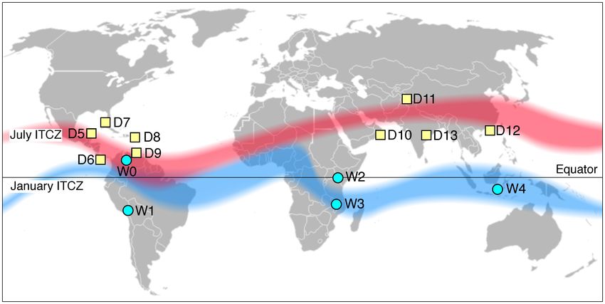
1       INTRODUCTION
The climate reflects a complex and dynamical interaction between the prevailing states of the atmosphere,
oceans, land masses, ice sheets and biosphere, in response to solar insolation. A climate transition in-
volves coupled changes of these systems following an initial perturbation, or “forcing”. The feedbacks
may be sufficiently strong that the net transition is substantially larger or smaller than from the forc-
ing alone. Nevertheless, it is important to identify the primary forcing agents since they provide the
fundamental reason why the climate changed, whereas the feedbacks determine by how much.
       Internal forcing agents (those arising within Earth’s climate system) include volcanoes, anthro-
pogenic greenhouse gases and, on very long time scales (tens of millions of years), plate tectonics.
Volcanoes have a cooling effect due to increased absorption and reflection of incoming shortwave radi-
ation by aerosols ejected into the stratosphere. Greenhouse gas concentrations determine the absorption
and emission of longwave radiation in the atmosphere with respect to altitude. Plate tectonics influence
the climate by changing the size, location and vertical profile of land masses, by modifying the air and
ocean circulations, and by exchanging CO2 in the atmosphere with carbonates in the lithosphere.
       At present, and ignoring meteor impact, there are only two established external forcing agents:
orbitally-modulated solar insolation and variations of solar irradiance. Spectral analysis of the glacial
cycles reveals precise frequencies that match Earth’s orbital variations caused by the gravitational per-
turbations of the other planets. In fact, the narrow spectral widths—obtained on untuned data—imply
that the glacial cycles are driven by an astronomical forcing agent, regardless of the detailed mechanism;
oscillations purely internal to Earth’s climate system could not maintain such precise phase coherency
over millions of years [1]. A linkage between orbit and climate is provided by the Milankovitch model,
which states that retreats of the northern ice sheets are driven by peaks in northern hemisphere summer
insolation. This has become established as the standard model of the ice ages since it naturally includes
spectral components at the orbital modulation frequencies. However, high precision palaeoclimatic data
have revealed serious discrepancies with the Milankovitch model that either fundamentally challenge its
validity or, at the very least, call for a significant extension [1].
       Variations of solar irradiance by about 0.1% have been measured over the 11 y solar cycle, and are
well understood in terms of sunspot darkening and faculae brightening [2]. From the knowledge of stellar
evolution and development, the slow progression of irradiance on extremely long time scales (of order
tens of millions of years) is also well understood. However, no mechanism has been identified so far
for secular irradiance variations on time scales between these two limits. On the other hand, substantial
magnetic variability of the Sun on decadel, centennial and millennial time scales is well established from
magnetometer measurements over the last 150 y [3] and from archives of 14 C in tree rings and 10 Be
in ice cores [4]. These light radioisotope archives record the galactic cosmic ray (GCR) flux in Earth’s
atmosphere, which is modulated by the interplanetary magnetic field and its inhomogeneities carried by
the solar wind. In earlier studies, long-term solar magnetic variability was assumed to be a proxy for
irradiance variability [5]. However this assumption lacks a physical basis, and more recent estimates
suggest that long-term irradiance changes are probably negligible [6, 7, 8].
       It is well-established that Earth’s climate varies substantially on centennial and millennial time
scales [9]. Some of these variations may be due to “unforced” internal oscillations of the climate system,
involving components with suitably long response times, such as the ice sheets. However, it is hard
to explain away all these climate variations as internal oscillations—especially in cases involving large
climate shifts (e.g. persistent suborbital variations of sea-level by 10–20 m have occurred during both
glacial and interglacial climates [10]), or where synchronous climate changes are observed in widely-
separated geographical locations, without any clear path for their teleconnection. At present there is
no established natural forcing agent on these time scales; they are either too short (solar irradiance,
volcanoes)1 or too long (solar insolation, plate tectonics). In recent years, however, numerous studies of
    1
        Greenhouse gases are not included since, prior to the twentieth century, short-term changes of greenhouse gases, such as

                                                                 1
centennial and millennial scale climate change have reported association with GCR variations. These are
frequently considered in the literature as a proxy for changes of solar irradiance (or a spectral component
such as solar ultra violet [12]). The ambiguous interpretation as either a solar-climate or a GCR-climate
forcing mechanism can in principle be resolved by examining climate change on different time scales
since, unlike solar irradiance, the GCR flux is also affected over longer times by geomagnetic and galactic
variations, and over shorter times by solar magnetic disturbances.
The complexity of the climate system means that it is not easy to explain correlations of solar
variability and climate in mechanistic models. On the other hand, the observations are too numerous and
of too high quality to be ignored or dismissed. The key challenge is to establish a physical mechanism
that could link solar or cosmic ray variability with the climate. If a detailed physical mechanism of
climatic significance were to be established then the whole field of solar variability would rapidly be
transformed into a quantitative and respectable branch of climate science. But what could the cosmic
ray-climate mechanism be? Since the energy input of GCRs to the atmosphere is negligible—about 10−9
of the solar irradiance, or roughly the same as starlight—a substantial amplification mechanism would
be required. An important clue may be the reported correlation of GCR flux and low cloud amount,
measured by satellite [13, 14, 15]. Although the observations are both disputed [16, 17, 18, 19, 20, 21]
and supported [22, 23, 24], increased GCR flux appears to be associated with increased low cloud cover.
Since low clouds are known to exert a strong net radiative cooling effect on Earth [25], this would
provide the necessary amplification mechanism—and also the sign of the effect: increased GCRs should
be associated with cooler temperatures.
Studying past climate variability, before any anthropogenic influence, is a good way to understand
natural contributions to present and future climate change. If there is good evidence for a significant influ-
ence of solar/GCR variability on past climate then it is important to understand the physical mechanism.
Despite the lack of evidence for long-term variability of the total or spectral (ultra violet) irradiance, it
cannot be ruled out and remains an important candidate. However since there is clear evidence for long-
term variability of cosmic rays, the possibility of a direct influence of cosmic rays on the climate should
also be seriously considered [26]. It is the purpose of this paper to review some of the palaeoclimatic
evidence for GCR-climate forcing—on progressively longer time scales—and to consider the possible
physical mechanisms and climatic signatures. Finally, we will describe how these mechanisms will be
studied under controlled laboratory conditions with the CLOUD facility at CERN.
2 SOLAR/COSMIC RAY-CLIMATE VARIABILITY
2.1 Last millennium
2.1.1 The Little Ice Age and Medieval Warm Period
The most well-known example of solar-climate variability is the period between 1645 and 1715 known
as the Maunder Minimum [27], during which there was an almost complete absence of sunspots (Fig. 1).
This marked the most pronounced of several prolonged cold spells between about 1450 and 1850 which
are collectively known as the Little Ice Age. During this period the River Thames in London regularly
froze across in winter, and fairs complete with swings, sideshows and food stalls were held on the ice.
The Little Ice Age was preceded by a mild climate known as the Medieval Warm period between about
1000 and 1270. Temperatures during the Medieval Warm period were elevated above normal, allowing
the Vikings to colonise Greenland and wine to be made from grapes in England.
A recent multi-proxy reconstruction of northern hemisphere temperatures [29] estimates that the
Little Ice Age was about 0.6◦ C below the 1961–1990 average, and that climate during the Medieval
Warm period was comparable to the 1961–1990 average (Fig. 2a). This contrasts with a widely-quoted
earlier reconstruction [31, 32], known as the hockey stick curve, which indicates a temperature decrease
occurred during glacial-interglacial transitions, are found to be a feedback of the climate system and not a primary forcing agent
[11].
2Fig. 1: Variation of the group sunspot number from 1610 to 1995 [28]. The record starts 3 years after the
invention of the telescope by Lippershey in Holland. The gradual increase of solar magnetic activity since the
Maunder Minimum is readily apparent.
Fig. 2: Comparison of variations during the last millennium of a) temperature (with respect to the 1961–1990
average), b) galactic cosmic rays (note the inverted scale; high cosmic ray fluxes are associated with cold temper-
atures) and c) glacial advances in the Venezuelan tropical Andes near Lake Mucubaji (8◦ 470 N, 70◦ 500 W, 3570 m
altitude) [30]. The temperature curves comprise a multi-proxy reconstruction of northern hemisphere temperatures
(the band shows 95% confidence interval) [29], the so-called hockey-stick curve [31, 32], borehole temperature
measurements worldwide [33] and from Greenland [34], and smoothed instrumental measurements since 1860.
The cosmic ray reconstructions are based on several 14 C measurements in tree rings (data points and dashed green
curve) [35, 36], and 10 Be concentrations in ice cores from the South Pole (solid blue curve) [37] and Greenland
(solid red curve) [38]. The 14 C anomalies are smaller than those of 10 Be since they are damped by exchanges with
the CO2 reservoirs.
3of only 0.2◦ C between 1000 and 1900, followed by a steep rise in the 20th century (Fig. 2a). However
the methodology of the hockey stick analysis has been questioned [39]. There have been numerous other
temperature reconstructions for the last millennium, which generally lie between these two limits, and
their unweighted mean is often used as the combined best estimate [8]. However, this can be misleading
since many of the reconstructions share the same temperature proxy datasets, so they are not independent
measurements. Perhaps the most accurate measurements of temperatures over the past millennium are
provided by geothermal data from boreholes, since these are direct measurements of past temperatures
with thermometers—albeit with a modest time resolution that does not preserve rapid changes. The
worldwide borehole measurements [33] indicate Little Ice Age temperatures about 0.6◦ C below those of
the mid-20th century, and the Greenland boreholes [34] indicate a pronounced Medieval Warm period
and Little Ice Age; all favour the multi-proxy reconstruction [29] shown in Fig. 2a.
For comparison, the variation of GCR intensity over the last millennium is shown in Fig. 2b, as
reconstructed from 14 C in tree rings [36], and 10 Be in ice cores from the South Pole [37] and Greenland
[38]. Close similarities are evident between the temperature and GCR records, showing an association
of high GCR flux with a cooler climate, and low GCR flux with a warmer climate. This pattern has been
extended over the last two millennia by a reconstruction of Alpine temperatures with a speleothem from
Spannagel Cave in Austria (Fig. 3) [40]. Temperature maxima in this region of central Europe during
the Medieval Warm Period were about 1.7◦ C higher than the minima in the Little Ice Age, and similar
to present-day values. The high correlation of the temperature variations to the ∆14 C record (Fig. 3)
suggests that solar/cosmic ray forcing was a major driver of climate over this period.
Fig. 3: Temperature reconstruction for the Central Alps over the last two millennia, obtained from the δ 18 O
composition of a speleothem from Spannagel Cave, Austria [40]. The variations of cosmic rays (∆14 C) and CO2
over this period are also indicated.
2.1.2 Intertropical Convergence Zone
Although the cultural records and temperature reconstructions of the Little Ice Age are predominantly
from Europe and the northern hemisphere, numerous palaeoclimatic studies have confirmed the cooling
to be a global phenomenon. One example which shows a clear GCR association is a reconstruction of
glacial advances in the Venezuelan tropical Andes (Fig. 2c) [30]. The inferred glacial advances indicate
this region experienced a temperature decline of (3.2±1.4)◦ C and a 20% increase of precipitation during
the Little Ice Age.
4Another example is a reconstruction of rainfall and drought in equatorial east Africa over the past
1100 y, based on the lake-level and salinity fluctuations of Lake Naivasha, Kenya [41]. The data show
that the climate in this region was significantly drier than today during the Medieval Warm period, and
that the Little Ice Age was an extended wet period interrupted by three dry intervals that coincide with
the GCR oscillations seen in Fig. 2b. A similar association of GCRs and tropical rainfall during the
Little Ice Age has been observed in the region of the Gulf of Mexico [42]. Increased GCR flux seems
to have paced increases in the salinity of the Florida Current, leading to a 10% reduction of the Gulf
Stream flow during the Little Ice Age. These examples suggest a possible solar/cosmic ray influence on
the Intertropical Convergence Zone (ITCZ). The ITCZ is a region of intense precipitation formed by the
convergence of warm, moist air from the north and south tropics by the convective action of the tropical
Hadley cells. The location of the ITCZ approximately follows the Sun’s zenith path, moving north in the
northern summer and south in the winter (Fig. 4). Numerous other palaeoclimatic reconstructions of the
Little Ice Age support the existence of a global influence of GCR flux on tropical rainfall and, moreover,
provide the rather clear picture that increased GCR flux is associated with a southerly displacement of
the ITCZ (Fig. 4) [43]. Since the deep convective ITCZ system is the major source of water vapour for
the upper troposphere in the tropics and sub-tropics, it controls the supply of the major greenhouse gas
(water vapour accounts for about 90% of Earth’s greenhouse effect [54]) and the availability of water
vapour for cirrus clouds over a large region. The displacement of the ITCZ during the Little Ice Age may
therefore imply a substantial global climate forcing.
Fig. 4: Locations of palaeoclimatic reconstructions of the Little Ice Age indicating wetter (circles labeled W0–
W4) or drier (boxes labeled D6–13) conditions than present [43]. The approximate most northerly (July) and
southerly (January) modern limits of the ITCZ are indicated by the wide transparent bands. The observations
indicate a southerly shift of the ITCZ range during the Little Ice Age. The references are W0 [30], W1 [44], W2
[41], W3 [45], W4 [43], D5 [46], D6 [47], D7 [42], D8 [48], D9 [49], D10 [50], D11 [51], D12 [52] and D13 [53].
2.1.3 Solar and cosmic ray changes since the Little Ice Age
The cold climate of the Little Ice Age appears to have been caused by an extended period of low solar ac-
tivity. Few sunspots implies low magnetic activity and a corresponding elevated GCR flux. But could the
observed warming since the Little Ice Age be explained by changes of solar irradiance rather than intro-
ducing the possibility of GCR-climate forcing? Recent results on Sun-like stars, combined with advances
in the understanding of solar magnetohydrodynamics [8] have revised earlier estimates of the long-term
variation of solar irradiance [5] downwards by as much as a factor of five (Fig. 5) [6, 7]. Apart from the
irradiance changes due to sunspot darkening and facula brightening, no mechanism has been identified
5Fig. 5: Top-of-atmosphere solar forcing since 1600 showing previous estimates (dashed curve) [5] and present
estimates (solid curve) [6].
Fig. 6: Variations of the 10 Be concentration in Greenland ice cores since 1700 (lower curve) [55] and of the solar
interplanetary magnetic field since 1870, derived from geomagnetic measurements (upper curve, note inverted
scale) [3]. The 10 Be concentration is directly proportional to the cosmic ray flux integrated over the troposphere
and stratosphere. The 10 Be data are unsmoothed, and their short-term fluctuations are dominated by solar cycle
modulation.
for solar luminosity variations on centennial or millennial time scales [8]. Current estimates of the sec-
ular increase of irradiance since 1700 are therefore based only on the variation in mean sunspot number.
The increase in irradiance amounts to less than 0.5 Wm−2 , which corresponds to about 0.08 Wm−2 at
the top of the atmosphere, globally averaged (Fig. 5). Assuming a climate sensitivity of 0.7 K/Wm−2 ,
this would contribute less than 0.06◦ C of the estimated 0.6◦ C mean global warming between the Maun-
der Minimum and the middle of last century, before significant anthropogenic contributions could be
involved.
On the other hand, there is clear evidence of a substantial increase in solar magnetic activity since
the Little Ice Age (Fig. 6) [55, 3]. The 10 Be record indicates that the mean global cosmic ray flux has
decreased by about 30% since the the Little Ice Age, with about one half of this decrease occurring
in the last century. The good agreement found between the 10 Be and 14 C records confirms that their
variations reflect real changes of the cosmic ray flux and not climatic influences on the transport processes
into their respective archives [56]. Around two-thirds of the 10 Be is produced in the stratosphere, and
one-third in the troposphere, so the ice cores archives are sensitive to relatively soft primary cosmic
6Fig. 7: Solar modulation of the galactic cosmic ray intensity for the period 1957–2001: a) balloon measurements
of the cosmic ray intensity at shower maximum (15–20 km altitude), measured by the Lebedev Physical Institute
[57, 58], and b) Wolf sunspot number. The curves correspond to four different locations for the balloon flights:
Mirny-Antarctica (0.03 GeV/c rigidity cutoff), Murmansk (0.6 GeV/c), Moscow (2.4 GeV/c) and Alma-Ata (6.7
GeV/c). Due to atmospheric absorption, the data of Murmansk and Mirny practically coincide with each other.
rays. The higher energy component that penetrates the troposphere has decreased by a smaller amount
than suggested by Fig. 6. During the twentieth century, the secular reduction of GCR intensity was
approximately equivalent to the present-day solar-cycle modulation (Fig. 6), corresponding to about 10%
in the troposphere. The decrease is due to an unexplained increase of the solar interplanetary magnetic
field by more than a factor of two over this period (Fig. 6) [3]. In view of the substantial variability of
cosmic rays, if they are indeed found to influence cloud cover it could have considerable implications for
understanding past climate change and predicting future variability.
During the second half of the twentieth century, the variation of GCR flux has been directly mea-
sured with particle counters. Although these instruments have a low threshold energy (few MeV) for
particle detection, the corresponding threshold energy of the primary cosmic rays depends on the type
of detected secondary particle and the amount of atmospheric shielding. In the case of ground-based
detectors at sea level, the primary proton threshold energy is about 1.5 GeV for neutron monitors and
about 9 GeV for ionization chambers (which detect muons, electrons and protons) [57]. The most sensi-
tive measurements are made by balloon-borne ionization chambers, which can reach 30–35 km altitude
(4 g/cm2 atmospheric shielding); these have a primary proton threshold of about 0.1 GeV at the highest
altitudes. The Lebedev Physical Institute has made continuous measurements of cosmic rays over the
last 50 years with balloon-borne detectors at several stations [57, 58]. The data for the period 1957–
2001 show the solar cycle modulation and the effect of geomagnetic shielding, which leads to reduced
fluxes and modulation amplitudes at lower geomagnetic latitudes (Fig. 7). Although the GCR reduction
7occurred mainly in the first half of the twentieth century (Fig. 6), the cosmic ray measurements shown
in Fig. 7 suggest a continuing decreasing trend in the second half of the century, by a few per cent in the
lower stratosphere and upper troposphere.
In summary, the estimated change of solar irradiance between the Little Ice Age and the mid
twentieth century is insufficient to explain the observed warming of the climate. Absence of evidence for
a long-term variation of solar irradiance does not, of course, rule it out; precision satellite measurements
of solar irradiance have only be available for the last 30 yr. On the other hand, there has been a substantial
increase of solar magnetic activity since the Little Ice Age, and a corresponding reduction of the cosmic
ray intensity. This suggests that the possibility of an indirect solar mechanism due to cosmic-ray forcing
of the climate should be seriously considered.
2.2 Holocene; last 10 ky
2.2.1 Ice-rafted debris in the North Atlantic Ocean
Evidence for millennial-scale climate variability during the Holocene has been found in the sediments
of ice-rafted debris in the North Atlantic [59, 60]. Deep sea cores reveal layers of foraminifera shells
mixed with tiny stones that were frozen into the bases of advancing glaciers and then rafted out to sea by
glaciers. These reveal abrupt episodes when cool, ice-bearing waters from the North Atlantic advanced
as far south as the latitude of southern Ireland, coincident with changes in the atmospheric circulation
recorded in Greenland. These so-called Bond events (named after their discoverer) have occurred with
a varying periodicity of 1470±530 y, during which temperatures dropped and glacial calving increased.
The estimated decreases in North Atlantic Ocean surface temperatures are about 2◦ C, or 20% of the full
Holocene-to-glacial temperature difference.
What could be the trigger for this millennial-scale climate change? Orbital variations of insolation
are too slow to cause such rapid changes. Ice sheet oscillations are also unlikely to be the forcing agent,
for two main reasons. Firstly, the icebergs were launched simultaneously from more than one glacier.
Secondly, the events continued with the same quasi-1500 y periodicity for at least the last 30 ky through
the Holocene and into the last glacial maximum (but with a larger amount of ice-rafted material)—even
though the ice sheet conditions changed dramatically over this interval. Solar/GCR variability appears
to be a promising candidate for the forcing agent during the Holocene phase since it is found to be
highly correlated with the Bond events (Fig. 8) [61]. Good agreement is seen between the 14 C (Fig. 8a)
and 10 Be (Fig. 8b) records, which confirms they are indeed measuring changes of the GCR flux, since
their respective transport processes from the atmosphere to archive are completely different. After its
formation, 14 C is rapidly oxidised to 14 CO2 and then enters the carbon cycle and may reach a tree-ring
archive. On the other hand, 10 Be attaches to aerosols and eventually settles as rain or snow, where it
may become embedded in a stable ice-sheet archive. The correlation between high GCR flux and cold
North Atlantic temperatures embraces the Little Ice Age, which is seen not as an isolated phenomenon
but rather as the most recent of around ten such events during the Holocene. This suggests that the Sun
may spend a substantial fraction of time in a magnetically-quiet state.
Coincident millennial scale shifts in Holocene climate have now been observed in regions far
from the North Atlantic. In the sub-polar North Pacific, variations of biogenic silica measured in the
sediment from Arolik Lake in a tundra region of south-western Alaska reveal cyclic variations in climate
and ecosystems over a 10 ky period that are coincident with the Bond events [62]. High GCR flux is
associated with low biogenic activity. In equatorial Africa, a 5.4 ky record of rainfall and drought in Lake
Edward indicates northward and southward displacement of the ITCZ in phase with the Bond events [63].
In southern China, analysis of a stalagmite from Dongge Cave has provided a continuous, high resolution
record of the East Asian monsoon over the past 9 ky [64]. Although broadly following summer insolation,
it is punctuated by 6–8 weak monsoon periods, each lasting 100–500 y, which coincide with the Bond
events. A high correlation is found over this entire period between the Dongge Cave monsoon record (5
y resolution) and the 14 C record (20 y resolution).
8Fig. 8: Correlation of GCR variability with ice-rafted debris events in the North Atlantic during the Holocene: a)
the 14 C record (correlation coefficient 0.44) and b) the 10 Be record (0.56), together with the combined ice-rafted-
debris tracers [61].
These results confirm the pattern seen in Fig. 4 for the Little Ice Age, and extend it throughout the
Holocene, namely a high cosmic ray flux is associated with a southerly displacement of the ITCZ. Taken
together, the observations suggest that solar/GCR forcing has been responsible for significant centennial
and millennial scale climate variability during the entire Holocene, on a global scale.
2.2.2 Indian Ocean monsoon
A high resolution record of the Indian Ocean monsoon over the period from 9.6 to 6.2 ky ago has been
obtained by analysing the δ 18 O composition in the layers of a stalagmite from a cave in Oman [65].
The δ 18 O is measured in calcium carbonate, which was deposited in isotopic equilibrium with the water
that flowed at the time of formation of the stalagmite. Oman today has an arid climate and lies beyond
the most northerly excursion of the ITCZ, which determines the region of heavy rainfall of the Indian
Ocean monsoon system. Stalagmite growth is evidence that the northern migration of the ITCZ reached
higher latitudes at earlier times. In this region, the temperature shifts during the Holocene are estimated
to account for only 0.25 per mil variation in δ 18 O [65], and so the δ 18 O variations are mainly due to
changes of rainfall. The data are shown in Fig. 9a, together with ∆14 C measured in tree rings such as
the California bristlecone pine. The two timescales have been tuned to match bumps within the known
experimental errors (smooth shifts have been applied to the U-Th dates up to a maximum of 190 y).
During a 430-y period centred around 8.1 ky BP, the stalagmite grew at a rate of 0.55 mm/y—an order
of magnitude faster than at other times—which allowed a high resolution δ 18 O measurement to be made
(Fig. 9b). The striking similarity between the δ 18 O and ∆14 C data indicates that that solar/GCR activity
tightly controlled the strength of the Indian Ocean monsoon during this 3,000-year period. Increased
GCR intensity is associated with a weakening of the monsoon (decreased rainfall) and a southerly shift
of the ITCZ, confirming with high time resolution the previous observations .
9Fig. 9: Profiles of δ 18 O from a U-Th-dated stalagmite from a cave in Oman, together with ∆14 C from tree rings
in California bristlecone pines and elsewhere, for a) the 3.4 ky period from 9.6 to 6.2 ky BP (before present) and
b) the 430 y period from 8.33 to 7.9 ky BP [65].
2.3 Quaternary; last 3 My
2.3.1 Stalagmite growth in Oman and Austria
There are two primary archives of past GCR changes: the 14 C record preserved in tree rings, and the
10 Be record in ice cores and ocean sediments. Since 14 C has a relatively short lifetime (τ
1/2 = 5730 y,
compared with 1.5 My for 10 Be), it is only useful for the period up to about about 40 ky ago. In order
to determine the atmospheric production rate of these radioisotopes (i.e. the GCR flux) from the mea-
sured concentrations in a particular climate archive, the transport effects between the atmosphere and
the archive must be accounted for. The transport of both 14 C and 10 Be is strongly influenced by differ-
ences between glacial and interglacial climates. Although 14 CO2 is well-mixed in the atmosphere, the
concentration is influenced by any changes in ocean ventilation or the extent of sea ice, since the deep
ocean is relatively 14 CO2 -depleted. In the case of 10 Be, changes in atmospheric circulation may sample
different latitudinal regions with different 10 Be concentrations. Moreover, the deposition flux depends
strongly on the relative rate of wet and dry deposition. For the present climate, the deposition flux of
10 Be in mid-latitude storm tracks is a factor 10 higher than over polar ice sheets, where dry deposition is
comparable to (Greenland) or even exceeds (Antarctic) wet deposition [66]. Extracting the 10 Be atmo-
spheric production rate from the measured flux into the ice sheets therefore has additional uncertainties
when large variations occur in the hydrological cycle and in the ice accumulation rates, such as during
glacial-interglacial transitions.
However, these difficulties are largely avoided in deep ocean sediments, where the 10 Be settling
time is about 1 ky, rather than the rapid (1 wk – 1 y) settling time onto the ice sheets. Although the
long settling time means the ocean archives are insensitive to rapid changes, it has the advantage of a
10Fig. 10: Comparison of the growth periods of stalagmites in Austria and Oman with a) 65◦ N June insolation and
b) the relative GCR flux (10 Be ocean sediments; note inverted scale) [68]. The growth periods are indicated by
shaded bands (Spannagel cave) or boxes (Hoti cave). Growth periods at Spannagel cave require warm temperatures,
close to the present climate; growth periods at Hoti cave require a moist climate. Periods without stalagmite growth
are unshaded. The dashed curves in b) indicate the estimated corrections of systematic errors in the SPECMAP
timescale, on which the GCR record is based. The growth periods appear to be associated with intervals of low
GCR flux, close to present values.
reduced sensitivity to regional variations of production or transport through the atmosphere, ensuring a
measurement of global GCR flux. A recent reconstruction of the global 10 Be production rate during the
last 220 ky using combined sediment cores from the Pacific, Atlantic and Southern Oceans shows that
the GCR flux was generally around 20–40% higher than today (Fig. 10b) [67, 68]. This is consistent
with palaeointensity reconstructions, both in sign and magnitude, which find an average geomagnetic
field strength over this period around 30–40% weaker than today [69]. It is also consistent with the
observed rise in 14 C production during the period from 10 ky to 45 ky before present, with roughly equal
contributions from the geomagnetic field changes and from changes in the global carbon cycle [70]. On
the other hand, a recent reconstruction [71] of the 10 Be flux for the last 50 ky from the Greenland ice
core finds no sign of any increase in the 10 Be flux between 10 ky and 30 ky before present, and attributes
the discrepancy to the 14 C data underestimating changes in the carbon cycle—although with large errors
that allow for changes of up to 20% in the production rate (GCR flux).
The ocean core 10 Be data show several 10–15 ky intervals over the last 220 ky when the GCR
flux returned to present levels (Fig. 10b). These changes are largely due to geomagnetic variability,
which is independently measured from palaeointensity data [69], although there may also be contribu-
tions from solar variability. During the periods of low GCR flux, stalagmite growth was observed in
caves located in Oman (Hoti cave) and Austria (Spannagel cave). In contrast, the stalagmite growth
periods show no clear pattern of association with 65◦ N June insolation, contrary to the expectations of
the standard Milankovitch model (Fig. 10a). The growth periods are precisely dated by U/Th analysis to
a 2σ precision of 1 ky (Spannagel) or 4 ky (Hoti). The growth of stalagmites at each of these locations
is especially sensitive to climate variations. In the case of Oman, water availability requires a warm
climate and monsoon rains. The observed growth periods of the Oman stalagmite extend the Holocene
observation shown in Fig. 9 back through the last two glaciations and interglacial—albeit with poorer
time resolution—namely, decreased GCR intensity is associated with a strengthening of the monsoon
11(increased rainfall) and a northerly shift of the ITCZ in summer. In the case of Austria, Spannagel cave
is situated at 2,500 m altitude in the Zillertal Alps, where the present mean air temperature is (1.5±1)◦ C.
Consequently, because of permafrost, stalagmites will not grow at Spannagel if the mean air temperature
outside the cave falls by only a small amount below present values.
Among the serious challenges to the Milankovitch model for the glacial cycles is the timing of
Termination II, the penultimate deglaciation. The growth period of stalagmite SPA 52 from Spannagel
Cave began at 135±1.2 ky BP [72] (Fig. 10b). So, by that time, temperatures in central Europe were
within 1◦ C or so of the present day. This corroborates the conclusion, based on sediment cores off the
Bahamas, that warming was well underway at 135±2.5 ky [73]. Furthermore, dating of a Barbados coral
terrace shows that the sea level had risen to within 20% of its peak value by 135.8±0.8 ky [74]. These
results confirm the “early” timing of Termination II, originally discovered at Devil’s Hole Cave, Nevada
[75]. This implies that the warming at the end of the penultimate ice age was underway at the minimum
of 65◦ N June insolation, and essentially complete about 8 ky prior to the insolation maximum (Fig. 10a).
The Milankovitch model therefore suffers a causality problem: Termination II precedes its supposed
cause. Furthermore, an analysis of deep ocean cores shows that the warming of the tropical Pacific Ocean
at Termination II preceded the northern ice sheet melting by 2–3 ky [76]. In short, orbital increases of
solar insolation on the northern ice sheets could not have driven the penultimate deglaciation—contrary
to the expectations of the Milankovitch model.
The 10 Be data, on the other hand, show that the GCR flux began to decrease around 150 ky, and had
reached present levels by about 135 ky (Fig. 10b). This is compatible with Termination II being driven
in part by a reduction of GCR flux—although the present 10 Be measurements have large experimental
errors. A similar reduction of GCR flux also occurred around 20 ky BP due to a rise in the geomagnetic
field strength towards present values. This coincides with the first signs of warming at the end of the last
glaciation, as recorded in the Antarctic ice at about 18 ky BP. Higher-precision 10 Be data from ocean
cores, extending to earlier times, are required to investigate this association more closely.
Despite the discrepancies with the Milankovitch model, it remains the only established mechanism
that could imprint the orbital frequencies on the glacial cycles. At present the GCR measurements from
the 10 Be record in ocean sediments have neither sufficient time span nor sufficient precision for spectral
analysis and a precise comparison with the orbital frequencies. Nevertheless, spectral analysis of the
GCR record during the last 220 ky (Fig. 10b) reveals two strong peaks consistent with orbital frequencies,
namely 0.01 c/ky (100 ky period) and 0.024 c/ky (41 ky) [77]. A higher-precision record of the GCR
flux over the past few hundred thousand years should in principle be available from the 10 Be record
in ice cores, but the challenge here is to disentangle real production rate changes from climate effects
on the transport of 10 Be into the ice. There are two possible mechanisms that could modulate GCR
ionisation with the orbital frequencies. Firstly, it is speculated that orbital variations could influence the
geodynamo, and thereby the GCR flux [78]. Some long-term records of Earth’s magnetic field suggest
the presence of orbital frequencies, in both strength and magnetic inclination [79, 80], but others do not
[69]. Secondly, as discussed later in this paper, it is plausible that lightning activity could be modulated
by the orbital insolation cycles. If so, this would modulate the ionospheric potential and the atmospheric
current density resulting from cosmic-ray ionisation in the atmosphere.
2.3.2 Laschamp event
If cosmic rays are indeed forcing the climate then there should be a climatic response to geomagnetic
reversals or excursions (“failed reversal” events during which the geomagnetic field dips to a low value
but returns with the same polarity). A relatively recent excursion was the Laschamp event, when the
geomagnetic field fell briefly to around 10% of its present strength and the global 10 Be production rate
approximately doubled [81]. Based on several independent radioisotope measurements, the Laschamp
event has been precisely dated at (40.4±2.0) ky ago (2σ error) [82].
No evidence of climate change was observed in the GRIP (Greenland) ice core during the Laschamp
12event [83]. However, this analysis applied a low pass filter to the 10 Be and climate (δ 18 O and CH4 ) mea-
surements, with a cutoff frequency of 1/3000 y−1 . This is substantially below the estimated 1500 y
duration of the Laschamp event [84] and has the effect of broadening (diluting) the signal region to
5.5 ky. When the GRIP data are viewed with higher resolution, the Laschamp 10 Be signal coincides with
a Dansgaard-Oeschger warming event (both the warming and cooling phases), and so it is difficult to
draw a firm conclusion on the absence or presence of an additional GCR-induced climate signal.
Several climatic effects coincident with the Laschamp event were recorded elsewhere. A pro-
nounced reduction of the East Asia monsoon was registered in Hulu Cave, China [85]. At the same
time, a brief wet period was recorded in speleothems found in tropical northeastern Brazil—a region that
is presently semi-arid [86]. The wet period was precisely U/Th dated to last 700±400 y from 39.6 to
38.9 ky ago; this was the only recorded period of stalagmite growth in the 30 ky interval from 47 to 16 ky
ago. Further evidence has recently been found in deep-sea cores from the South Atlantic, by analysing
Nd isotopes as a sensitive proxy of the thermohaline ocean circulation [87]. A brief, sharp reduction of
North Atlantic deep water (NADW) production was recorded (i.e. towards colder conditions), coincident
with the Laschamp event.
This pattern of climate response to the Laschamp excursion of little or no signal at high latitudes
(Greenland) but possible signals at low latitudes (China, Brazil, NADW—perhaps reflecting Gulf Stream
salinity changes) is consistent with what could be expected from a geomagnetic dip. For a primary cos-
mic ray to produce ionisation in the lower troposphere, it must create a secondary muon of at least 2 GeV
to have sufficient energy to pass through the atmosphere. This implies a primary proton energy of at least
about 9 GeV which, for the present geomagnetic field, corresponds to the geomagnetic cutoff at a latitude
of about 40◦ . So, for Greenland (which lies above 60◦ N), the cosmic ray flux in the lower troposphere is
presently limited by the atmospheric column density and not by the geomagnetic field strength. Even a
large reduction of the geomagnetic field—such as during the Laschamp event—would not significantly
increase the lower tropospheric ionisation over Greenland (although it would produce a large spike in
10 Be, as observed [83], since this reflects the combined tropospheric and global stratospheric ionisation).
The regions that would first be affected by a geomagnetic dip are at low latitudes, where the tropospheric
ionisation is presently limited by the geomagnetic cutoff; these are indeed the regions that seem to in-
dicate some climate correlations with the Laschamp event. Higher latitudinal regions could be affected
later in response to the low-latitude climate changes. However, the short duration of the Laschamp event
may not have been sufficient to allow for significant additional cooling to take place at the latitudes of
the northern ice sheets, which were already under predominantly-glacial conditions.
2.4 Phanerozoic; last 550 My
2.4.1 Celestial cycles
Tropical sea surface temperatures throughout the Phanerozoic have been reconstructed from the δ 18 O of
calcite and aragonite shells found in ocean sediments (30◦ S–30◦ N) [88]. After detrending and smoothing
the data, the reconstructed temperatures (Fig. 11b) show an oscillating behaviour that matches reasonably
well with Earth’s icehouse and greenhouse climate modes, established from sediment analyses elsewhere
(indicated at the top of Fig. 11).
Independently, a correlation was noted between the occurrence of ice-age epochs on Earth and
crossings of the spiral arms of the Milky Way by the solar system, during which elevated GCR fluxes
of up to a factor of two are estimated (Fig. 11a) [89]. The GCR flux is higher within the spiral arms
owing to the relative proximity of the supernovae generators and the subsequent diffusive trapping of
the energetic charged particles by the interstellar magnetic fields. The estimated crossing periodicity of
about 140 My is supported by the GCR exposure age recorded in iron meteorites [89]. Both the GCR
flux and ocean temperatures appear to follow the same cyclic behaviour and the same phase (Fig. 11b),
whereas estimated CO2 levels do not [90]. These observations have been both disputed [91, 92] and
supported [93, 94]. However, on quite general grounds, it is hard to conceive of anything other than a
13Fig. 11: Correlation of cosmic rays and climate over the past 500 My [90]: a) GCR mean flux variations as the
solar system passes through the spiral arms of the Milky Way, reconstructed from iron meteorite exposure ages
[89], and b) ocean temperature anomalies reconstructed from δ 18 O in calcite shells found in sediments from the
tropical seas [88]. Panel a) shows the nominal reconstructed GCR flux (black curve) and the error range (grey
band). The dashed red curves in panels a) and b) shows the best fit of the GCR flux to the temperature data (solid
blue curve in panel b), within the allowable error (note inverted GCR scale in panel b). The data are de-trended
and smoothed. The dark bars at the top represent cool climate modes for Earth (icehouses) and the light bars are
warm modes (greenhouses), as established from sediment analyses elsewhere.
galactic mechanism to account for a 140 My periodicity.
Higher frequency components of the temperature data in Fig. 11b have also been analysed [95].
Significant power is found at 34 My period, and this matches both the estimated phase and period
(34±6 My) for crossings of the galactic plane by the solar system. This motion corresponds to oscilla-
tions above and below the galactic plane with a full cycle of 64–68 My [94, 95]; and it is independent of
the motion in the galactic plane, as analysed in ref. [89].
An alternative mechanism has been proposed to explain these apparently galactic-related period-
icities. When passing through the spiral arms of the galaxy, as well as experiencing a higher cosmic ray
flux, the solar system encounters giant molecular clouds [96]. These are the remnants of supernovae, and
comprise 99% gas and 1% dust grains. In extreme cases the clouds may reach densities as high as 2000
H atoms cm−3 . This may be compared with about 0.3 H atoms cm−3 in the present local interstellar
cloud which, nevertheless, gives rise to about 40,000 tons of extraterrestrial matter falling on Earth’s sur-
face each year. Passage through high density interstellar clouds would cause the heliosphere to collapse
below 1 AU, exposing the stratosphere to large quantities of interstellar dust and potentially triggering a
“snowball” glaciation on Earth by radiative forcing [97]. Collapse of the heliospheric shield would also
lead to a large increase of GCR flux on Earth; the 10 Be rate is estimated to increase up to 400% of the
present value [98]. Thankfully, present estimates suggest that the frequency of encounter of the solar
system with an interstellar cloud of >2000 H atoms cm−3 is rather low (of order one per Gy).
2.4.2 Biodiversity
The diversity of life during the course of the Phanerozoic has fluctuated. Analysis of the fluctuations
of the number of marine genera has revealed a strong (62±3) My cycle and a weaker cycle at 140 My
[99]. The 140 My cycle may be associated with the GCR-climate cycle, but cold periods in δ 18 O precede
14the 140 My diversity maxima by 20–25 My. The stronger 62 My cycle does not have any clear origin
(a GCR effect due to the vertical oscillation relative to the galactic disk should show up as a 34 My
cycle). Using databases covering the Precambrian (4500–543 My ago) and Phanerozoic, an independent
measurement of the biodiversity fluctuations has been made from changes of the biological tracer, δ 13 C
[100]. These show a remarkable agreement with the reconstructed GCR flux over a 3.5 By period, based
on the expected solar evolution and rate of formation in our galaxy of massive stars that ended life as
supernovae.
An alternative way in which the galactic environment could affect cosmic rays and biodiversity
is through isolated events, namely nearby Type IIa supernovae, which could produce a “cosmic ray
winter” [101]. Around one such event is expected per My at a distance of a few × 10 pc. The first direct
evidence for a close supernova explosion has recently been obtained from an enhancement in the fraction
of the 60 Fe radioisotope (τ1/2 = 1.5 My) in a deep-sea ferromagnetic crust [102]. The measurements
unambiguously show the presence of a nearby supernova that occurred 2.8 My ago; the 60 Fe amounts
are compatible with a distance of a few × 10 pc. This is estimated to have increased the GCR flux by
around 15% for a period of about 100 ky. Under the assumption of GCR-climate forcing, this would
have caused a prolonged cold period; coincidentally or not, the onset of northern hemisphere glaciation
occurred at the same time.
3 MECHANISMS
3.1 GCR-cloud mechanisms
3.1.1 GCR characteristics
Galactic cosmic rays mainly comprise high energy protons which have been accelerated by supernovae
and other energetic sources in the Milky Way galaxy. The main flux is in the energy region of a few
GeV, although the spectrum extends eleven orders of magnitude higher (albeit with negligible intensity).
The primary cosmic rays interact in the atmosphere at around 30 km altitude, producing showers of
secondary particles which penetrate the troposphere; below 7 km, the secondaries are mainly muons.
The charged cosmic rays lose energy by ionisation and, away from continental sources of radon, are
responsible for essentially all of the fair-weather ionisation in the troposphere. Ion-pair production rates
vary between about 2 cm−3 s−1 at ground level, 10 cm−3 s−1 at 5 km, and 20–50 cm−3 s−1 at 15 km
altitude, depending on geomagnetic latitude. Taking into account production rates and loss mechanisms
such as recombination and attachment to aerosols, the equilibrium ion pair concentrations vary between
about 200–500 cm−3 at ground level and 1000–3000 cm−3 in the lower stratosphere [103]. The GCR
flux is modulated (typically by a few tens of per cent, depending on latitude and altitude) by the solar
wind, the geomagnetic field strength and the galactic environment of the solar system. Since these vary
over periods from tens to billions of years, a putative GCR-climate forcing has the potential to affect
climate on all time scales.
Two different classes of mechanisms have been proposed to link the GCR flux with clouds. The
first hypothesis is that the ionisation from GCRs influences the production of new aerosol particles in
the atmosphere, which then grow and may eventually increase the number of cloud condensation nuclei
(CCN), upon which cloud droplets form. The second hypothesis is that GCR ionisation modulates the
entire ionosphere-Earth electric current which, in turn, influences cloud properties through charge effects
on droplet freezing and other microphysical processes.
3.1.2 Ion-induced nucleation of new aerosols
Aerosols are continuously removed from the atmosphere by wet and dry sedimentation, by self coagu-
lation, and by scavenging in clouds. As a result they have short lifetimes—of order a day—and the rate
at which new aerosols are produced can have a large influence on clouds. An important source of new
aerosols is thought to be nucleation from trace condensable vapours in atmosphere, but these processes
15remain poorly understood [104]. The atmosphere contains very few trace gases that are suitable for nu-
cleation; the most important is thought to be sulphuric acid, although ammonia and iodine oxides may
also be significant. However, the concentration of sulphuric acid in the atmosphere is generally too low
to drive the subsequent growth to CCN sizes. Over land masses, organic compounds such as acetone
and the oxidation products of terpenes emitted by trees are thought to be important for aerosol growth.
In marine regions, isoprene oxidation products and iodine oxides are thought to participate in aerosol
growth.
Fig. 12: Ion-induced nucleation of new particles from trace condensable vapours and water in the atmosphere.
New aerosols consist of small clusters containing as few as two molecules (Fig. 12). These may
grow by further condensation of molecules of trace vapours and water—or they may evaporate. Above
a certain critical size, the cluster is thermodynamically more likely to grow by further condensation;
below the critical size, it is more likely to shrink by evaporation. The presence of charge stabilises the
embryonic cluster through Coulomb attraction, and reduces the critical size—a process known as ion
induced nucleation [105, 106, 107].
As well as inducing particle formation, charge also accelerates the early growth process, due to
an enhanced collision probability, and thereby increases the fraction of particles that survive removal by
coagulation before reaching sizes of 5 nm [108]. Beyond this size, electrostatic effects are thought to be
negligible, but coagulation rates also fall strongly due to the lower particle mobility. So, with regard to
enhancing the survival of new particles to CCN sizes, charge operates precisely in the most critical range,
below 5 nm. Nevertheless, only a small fraction of new particles reach the minimum size to be effective
CCN (about 50 nm), since most are lost by scavenging on existing aerosols. Geographical regions of
very low pre-existing aerosol loading are therefore the most favorable for growth of fresh CCN from
new particle production.
Particle formation in the upper troposphere tends to occur readily since the condensable vapours
are often supersaturated (due primarily to the low ambient temperatures and the small pre-existing aerosol
surface area). In the boundary layer, however, nucleation tends to occur during “aerosol bursts”, char-
acterised by long periods without any new production followed by brief periods of rapid production and
growth lasting a few hours. These bursts presumably occur when the threshold conditions, such as trace
vapour concentrations, are reached so that nucleation and/or growth to detectable sizes [109] can take
place. In ion induced nucleation models, the presence of charge from GCRs lowers this threshold. The
16observed particle production rates are typically in the range 0.1–10 cm−3 s−1 , although they may be as
high as 104 cm−3 s−1 or more [104]. In the lower troposphere the ion pair production rate from GCRs
is about 5 cm−3 s−1 and the equilibrium small ion concentration is about 500 cm−3 , so only some of
the nucleation events could be readily explained by ions. A further complication in assessing the contri-
bution of ions to nucleation bursts is that the counting threshold of present instruments is 3 nm aerosol
size, whereas the nucleation occurs around 0.5 nm. A large but uncertain fraction of new particles may
therefore be lost by coagulation before they are detected, so the true nucleation rate has not yet been
measured [110]. In addition, a large population of neutral ultrafine aerosol may exist below the 3 nm
threshold, whose growth is inhibited due to lack of condensable vapours [109]. In this case, it is possible
that ion induced nucleation could slowly populate the ultrafine aerosols over an extended time, allowing
a mechanism for large aerosol bursts that exceed the instantaneous ion-pair production rate from GCRs.
There is some experimental and observational evidence to support the presence of ion induced
nucleation in the atmosphere. Early studies, beginning in the 1960’s, [111, 112] demonstrated ultrafine
particle production from ions in the laboratory, at ion production rates typically found in the lower
atmosphere. This has also been found in a more recent laboratory experiment, under conditions closer to
those found in the atmosphere [113]. Observations of ion-induced nucleation in the upper troposphere
have also been reported [114, 115] and also of aerosol bursts in the lower troposphere [116], although
their rate frequently exceeds what could be caused by instantaneous ion-induced nucleation. Laboratory
measurements have shown that ions are indeed capable, under certain conditions, of suppressing or even
removing the barrier to nucleation in embryonic molecular clusters of water and sulphuric acid at typical
atmospheric concentrations, so that nucleation takes place at a rate simply determined by the collision
frequency [117, 118, 119].
3.1.3 Global electric circuit
The second mechanism that may link GCR flux and clouds concerns the effect of GCRs on the global
electric current flowing between the ionosphere and Earth’s surface [120, 121]. Except for a contribution
from radioactive isotopes near the land surface, GCRs are responsible for generating all the fair-weather
atmospheric ionisation between ground level and the mid mesosphere, at about 65 km altitude. As such,
GCRs fundamentally underpin the global electrical circuit.
The atmospheric electric circuit involves a global current of about 1400 A (and 400 MW power)
which is sustained by thunderstorms continuously active over tropical land masses (Fig. 13) [122, 123].
The thunderstorms carry negative charge to the ground and an equivalent positive current flows up to the
ionosphere. Due to the high currents, large electric fields are generated above thunderstorms and the air
can break down electrically to produce optical flashes known as sprites and elves. This current generator
maintains the ionosphere at a relative positive potential of about 250 kV. The return current between
the ionosphere and the Earth’s surface flows throughout the atmosphere, in regions of disturbed and
undisturbed weather, and is carried by vertical drift of small ions; the average fair-weather vertical current
density, Jz , is 2.7 pA m−2 [122, 123]. By controlling the lower atmospheric ion pair concentration, GCRs
can affect Jz , the atmospheric conductivity, the ionospheric potential, and the vertical potential gradient
in the atmosphere. In polar regions, these quantities are also influenced by low energy ionising particles
from relativistic (∼1 MeV) electron precipitation, which may occur during crossings of the solar wind
magnetic sector boundaries.
Decadel changes in the ionospheric potential and surface potential gradient have in fact been ob-
served and attributed to changes in the GCR flux [124, 125]. The positive correlation observed between
GCR flux and surface potential gradient [125] would imply an influence on the current source in order
to sustain the higher net flow of fair-weather charge through the atmosphere, which, at the same time,
has a higher conductivity. The simplest explanation is that the GCRs affect the conductivity or electrical
breakdown between the top of thunderstorms and the ionosphere; increased GCR flux could then lead to
increased current generation.
17You can also read